Integrated Simulation System for 5-axis Milling Cycles

(1)

Peer-review under responsibility of the International Scientific Committee of the “15th Conference on Modelling of Machining Operations doi: 10.1016/j.procir.2015.03.057

Procedia CIRP 31 ( 2015 ) 64 – 69

ScienceDirect

15th CIRP Conference on Modelling of Machining Operations

Integrated simulation system for 5-axis milling cycles

Tunc L.Taner

a*

_{, Sulitka Matej}

b

_{, Kopacka Jan}

b

a_{Nuclear AMRC, University of Sheffield, Advanced Manufacturing Park, Brunel Way, Sheffield, S60 5WG, United Kingdom} b_{Czech Technical University, Faculty of Mechanical Engineering, RCMT, Horská 3, 128 00 Praha 2, Czech Republic} * Corresponding author. Tel.: +44-1142-226676 ; E-mail address: [email protected]

Abstract

Multi axis milling is a promising technology for machining of complex geometries and surfaces. Thanks to the additional rotary axis, it provides flexibility to overcome the accessibility issues. However, the process becomes more complicated in terms of geometry, mechanics and dynamics due to the additional degrees of freedom and ball nose end mills. In this study, mechanics and stability of 5-axis ball end milling operations is simulated throughout a given toolpath. The cutting tool-workpiece engagement boundary is calculated and workpiece is represented using distance field approach. Distance field approach features very low computational time, close to real-time simulation. The cutting forces are modeled using orthogonal-to-oblique transformation. Stability limits are estimated in frequency domain.

Peer-review under responsibility of The International Scientific Committee of the “15thConference on Modelling of Machining Operations”. Keywords: Stability; Simulation; Milling; Geometric Modelling; Dynamics

1.Introduction

5-axis milling is widely used in manufacturing of parts with complex geometries, where part quality and productivity is very critical considering the high cost of the equipment and material involved. Several types of materials are machined such as aluminum, steel and titanium in such industries each of which has unique behavior in cutting. As 5-axis milling became an established process technology in the last decades there are several alternatives for tooling and cutting parameters to be selected in process development stage. Considering the complex geometry, mechanics and dynamics of milling, it is very important to develop and apply process models for such purposes [1-3]. The existing virtual process simulation systems and models are summarized by Altintas et al. in a recent CIRP keynote paper [1], where it is also emphasized that simulation of 5-axis milling cycles requires integration of workpiece representation models, proces models, and tool-workpiece engagement calculation methods.

Modelling of the cutting forces, where geometry of process and tool are defined together with chip thickness, is the first step in simulation of machining processes. Extensive amount of work has been done on modeling of milling mechanics for

different tool types. Lee and Altintas [4] modeled the mechanics and dynamics of helical ball end mills employing orthogonal to oblique transformation [5]. Later, Engin and Altintas [6,7] proposed the first model for mechanics and dynamics of 3-axis milling with generalized cutters, where helical cutting edges are modeled to be wrapped around the tool envelope. Ozturk and Budak [8] proposed one of the first models for estimation of cutting forces in 5-axis ball end milling. They modeled the engagement boundary and chip thickness considering the tool orientation with respect to the workpiece surface and verified the simulations through experiments. In a recent study Kaymakci et al. [9] developed a unified mechanistic model for turning, boring, drilling and milling where transformation to the cutting edge is applied with respect to the process in focus. Tunc et al. [10] proposed a generalized cutting force model for 5-axis milling with generalized definition of cutter envelope and cutting edge.

It is well known that stability diagrams are helpful for selection of chatter-free cutting conditions. There have been several studies on modeling of chatter stability in milling. In one of the early studies Koeningsberger ant Tlusty [11] applied orthogonal chatter stability model on 2½ end milling by employing an average cutting direction and average number of

(2)

teeth in cut. Later, Opitz and Bernardi [12] improved that approach by employing variable directional coefficients. End milling is considered as a 2-DOF system by Minis et al. [13], leading to more accurate estimation of stability limits, where

Floquet’s theorem and Fourier series are used for the stability

solution based on Nyquist stability criterion. Budak and Altintas [14] propose the first analytical solution to the milling stability problem, where single and multi-frequency solutions are applied. As one of the first attempts on modelling of ball-end milling stability, Altintas et al. [15] applied single-frequency solution to 3-axis ball-end milling. Ozturk et al. [16] extended this approach to 5-axis ball end milling through an iterative multi-frequency method. Modeling of milling stability with irregular cutting edges such as serrated [17-19], variable helix and variable pitch [20] forms are also studied.

Besides modeling the process mechanics and dynamics, representation of workpiece geometry throughout the machining cycle is essential for machining cycle simulation. To prevent the complexity of direct solid modelling to represent a workpiece volume it is more effective to use spatial decomposition. Most common and robust numerical models used to represent the workpiece is the dexel – based technique (also called Z-mapping technique) or the voxel – based method. The dexel method is given by discretizing an initial workpiece volume by a set of vectors, parallel to the z-axis of three dimensional coordinate system and located at the two dimensional square grid of x-y plane, presented in a variety of papers [22], where the overall accuracy is determined by the grid scale. Disadvantage of this method is, when the surface inclination gets too steep and the surface normals are nearly perpendicular to the grid vectors, accuracy of the surface representation becomes very poor. An option to remedy this is to incline the vectors in each point of the workpice final surface according to the surface normal [25]. Another possible approach applies additional sets of vectors parallel to –x and/or

–y directions. The final conclusion is a multi – dexel volume that represents the workpiece surface in an optimal quality for virtual machining [26][27]. The workpiece is updated throughout the simulation by updating the vector lengths through intersection with cutter tool body.

On the other side, in voxel – based method the workpiece is decomposed into a collection of basic geometric elements, mostly axis aligned cubic parts [28],[29]. Modelling using voxel elements is mainly done by creating octree data structure in detail [30], [31]. Accuracy of this method is given by the element sizes. Each cube can be divided into 8 smaller cubes to form octants and sub-octants etc. Voxel method allows to represent and update the in-process workpiece by simple Boolean subtraction. A refinement to the voxel method is the distance field technique, which maps a point in space (voxel node) to its shortest distance point on a surface [32]. In [33], material removal simulation and machined surface quality is obtained as the Boolean difference between distance field representing the original workpiece volume and distance fields representing the volumes of the milling tool swept along the milling path.

As summarized in this section the two main elements towards milling cycle simulation are the process models and workpiece representation. However, both of these require

different expertise. Process modeling requires expertise and understanding in mechanics, geometry and dynamics of cutting. However, representation of workpiece geometry requires expertise in computer graphics and geometrical modeling. The workpiece representation calculates the engagement boundaries and the process modeling techniques uses this information to simulate the process. At this point, these two modules need to be integrated through a standard data transfer format. There are couple of commercial integrated

machining simulation systems such as MachPro © [34] and

Machining Studio © [35].

In this study, such two modules are integrated for simulation of 5-axis milling cycles to develop an integrated machining cycle simulation system, which is capable of simulation of cutting forces and stability limits. Henceforth, the paper is organized as follows; the next section briefly describes the geometry of 5-axis milling. Then, the distance field approach, used for workpiece representation and determination of engagement boundaries, is given. In Section 4, mechanics and dynamics of milling briefly presented. The paper is finalized with experimental results and conclusions.

Nomenclature

r(z) local radius of the cutting tool

Ԅ୨ሺሻ local immersion angle

Ȱ tool rotation angle

ɗ୨ሺሻ radial lag angle

j index of the cutting edge

݀ߙ angular discretization step dz axial discretization step

Kic axial, radial, tangential cutting force coefficient Kie axial, radial, tangential edge force coefficient

୨ instantaneous chip thickness

୲ feed per tooth per revolution dSj The differential cutting edge length H convergence criteria

y orthogonal projection of a point in 3D space d(x) distance field function

S surface of the object could be represented ds(x) the signed distance function

dFij Differential cutting forces in direction i at tooth j

ߜሺݖሻ Kronecker delta function

CEB Cutter engagement boundaries in tool coordinates alim Stability limit

p index of the CL point 2.Geometry of 5-axis milling

In 5-axis milling, 3 coordinate systems i.e. machine coordinate system (MCS), process coordinate system (FCN) and tool coordinate system (TCS) are used to define the process geometry (see Fig. 1a). MCS is fixed to the –X, –Y and –Z axis of the machine tool. FCN consists of the feed (F), cross feed (C) and normal (N) of the machined surface. Finally, the tool axis vector forms the TCS together with two vectors transversal to the tool axis. Rotation of the tool axis around feed and cross feed directions enables different tool geometries for contouring purposes. Thus, the generalized tool geometry definition [10]

(3)

is used in this study, which consists of cone, torus, taper and cylinder. Different types of cutters can be obtained by combination of these parameters.

(a) Coordinate systems (b) Top view. Fig. 1: General milling tool geometry [10].

A point P(z) on a cutting edge is defined in cylindrical coordinates in terms of radial distance r(z), the radial lag angle

ψ(z) and the axial immersion angle κ(z), i.e. the angle between the tool axis and the cutting edge normal (see Fig. 1b). There is rotational lag angle, ψ(z), between consecutive points on the cutting edge due to helix angle. The immersion angle of any point is written in terms of the lag angle and the cutter rotation angle, ϕ. For general milling tools with variable helix and variable tooth pitch separation, the generalized local immersion angle ϕj(z) for the jth cutting edge is written as follows [10];

߶௝ሺݖሻ ൌ ߶ ൅ ߶௣ǡ௝െ ߰௝ሺݖሻ (1) where,ϕp,j and ψjare the pitch angle of the jth cutting edge with

respect to the previous one and the axial lag angle of the jth

cutting edge at level z, respectively.

3.Modeling of process geometry using distance fields

3.1.Workpiece representation

A distance field ݀ǣ ൌ Թଷ_{՜ Թ}_{is a scalar function of space} coordinates which returns the shortest distance to an object. The object is described by a domain ȳ with boundary μȳ. The distance is most commonly measured by the Euclidian metric, here denoted by ԡڄԡǤ The foot point ܡത א μȳ, i.e. the orthogonal projection of a point ܠ א Թଷ_{onto the object surface, is obtained} as the minimizing argument.

࢟

ഥሺ࢞ሻ ൌ ܽݎ݃ ݉݅݊௬אడఆԡ࢞ െ ࢟ԡ (2) The distance function then easily arises as

݀ሺ࢞ሻ ൌ ԡ࢞ െ ࢟ഥሺ࢞ሻԡ (3)

Having the distance function at hand, the surface of the object can be represented as the zero level of this function

ܵ ൌ ሼ࢞ א Թଷ_{ȁ݀ሺ࢞ሻ ൌ Ͳሽ} (4)

However, the distance function (2) does not carry information whether a point ࢞ lies inside or outside of the object. Therefore, the signed distance function is introduced

݀௦ሺ࢞ሻ ൌ ݏ݅݃݊ሺ࢞ሻ݀ሺ࢞ሻ (5)

The signum function ݏ݅݃݊ሺܠሻ is calculated as follows

ݏ݅݃݊ሺ࢞ሻ ൌ ሺ࢞ െ ࢟ഥሺ࢞ሻሻ ڄ ࢔

ԡሺ࢞ െ ࢟ഥሺ࢞ሻሻ ڄ ࢔ԡ (6)

where ࢔ is the unit outward normal vector of the surface. The signum function returns plus one if ܠ is outside the object and minus one if ܠ is inside the object. Note that zero value indicates zero distance so that sign is irrelevant in this case.

Fig. 2: A surface representation by the signed distance field sampled on the sparse block grid data structure ([32]).

For simple shapes the signed distance field can be expressed analytically. However, for more complex shapes it needs to be treated numerically. In practice, values of signed distance are sampled into discrete points near the object surface. The discrete points can be spread in regular grid (i.e. voxel grid), or in a more sophisticated sparse block grid data structure which is depicted in Fig. 2 When a value of ݀ୱሺܠሻ is required, it is reconstructed from nearby samples using the trilinear interpolation. A particular implementation of distance field as well as description of the sparse block grid data structure were presented in reference [32].

3.2.Calculation of engagement boundaries

The distance field representation of a geometry makes the calculation of the engagement region relatively quick. Regular voxel grid of the distance-field enables an implementation of a fast querying whether a particular point lies inside or outside of the workpiece. Such procedure is usually implemented already in the visualization of the workpiece as it is essential for rendering. The principle of the procedure for a 2D case is depicted in Fig. 3a. Let us consider a generic point given by its coordinate x. One can determine the voxel indices simply as the integer part of the fraction ݔ௜Ȁ݄௜, where ݅ is the index of a spatial dimension. Once the affected voxel is known, its distance field can be evaluated and the final identification can be made whether the point is in the workpiece.

The procedure described is repeatedly called for each of the discrete points of the tool as depicted in red dotes in Fig. 3b. The discrete points are constructed as regularly spaced rings along the tool axis with pitch dz. The rings are formed by points on the tool with the constant angular spacing, dα. An example of engagement region is shown in Fig. 3b. Tool engagement boundary is visualized together with the color scale depicting the instantaneous chip thickness at each point. Indeed, the accuracy of the engagement region assessment depends on the spacing parameters dz and dα.

(4)

(a) Tool envelope

(b) Engagement boundaries Fig. 3: Discretized tool envelope in 2D.

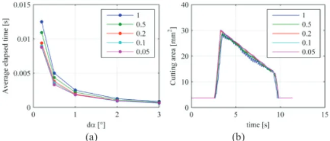
The computation efficiency is evaluated through the average computational time of the engagement region in Fig. 4a. The axial spacing is dz = 0.2 mm and only the angular spacing, dα, is varied. Also different density of the workpiece voxel grid from 0.05 mm to 1 mm is considered. It is observed that the computation time does not significantly depend on the voxel grid density. Besides, it is seen from Fig. 4a, that even for angular spacing equal to 1 degree the average computation time is approximately 2 ms, which reveals the potential of the distance field based engagement boundary calculation procedure for the on-the-fly calculation.

Accuracy of the contact area calculation within the engagement boundaries as a function of the voxel grid density for a given tool path is shown in Fig. 4b. The calculation is done for the value of dz = 0.2 mm; tool diameter is 5 mm. It can be seen that reducing the voxel grid spacing below 0.5 mm brings no more substantial differences in the calculated values of the tool contact area.

(a) (b)

Fig. 4: (a) Computation performance vs angular discretization (b) Accuracy performance of distance field based calculation.

4.Mechanics and dynamics of 5-axis milling

Modelling of milling processes requires the chip thickness to be defined and related to the either static or dynamic cutting forces. The engagement boundary information is used to calculate the chip thickness and chip regeneration for cutting force and stability simulation, respectively. In this section, mechanics and dynamics of 5-axis milling is summarized based on previous models [10], [16].

4.1.Modeling of cutting forces

Once the engagement boundaries are known the cutting forces are modelled using oblique-to-orthogonal cutting transformation [10]. The differential cutting forces acting at a point P on the jth_{cutting edge are calculated by knowing the} local chip thickness. Differential cutting forces in the radial, axial and tangential directions on an axial disc of the jth_tooth at elevation

z

and at rotation angle ϕj are calculated according to the mechanistic model [4]. Then, the differential cutting forces are summed up along the cutting tool axis.

൦ ݀ܨ௥ೕሺݖሻ ݀ܨ௧_ೕሺݖሻ ݀ܨ௔ೕሺݖሻ ൪ ൌ ൦ ܭ௥௖݄௝൫߶௝ǡ ݖ൯ܾ݀ ൅ ܭ௥௘݀ܵ௝ ܭ௧௖݄௝൫߶௝ǡ ݖ൯ܾ݀ ൅ ܭ௧௘݀ܵ௝ ܭ௔௖݄௝൫߶௝ǡ ݖ൯ܾ݀ ൅ ܭ௔௘݀ܵ௝ ൪ ή ߜሺݖሻ where, ߜሺݖሻ ൌ ቊͳ݂݅ܲሺݖǡ ߶௝ሻ א ܥܧܤሺ߶ǡ ݖሻ Ͳ݂݅ܲሺݖǡ ߶௝ሻ ב ܥܧܤሺ߶ǡ ݖሻ (7)

4.2.Dynamics and stability of 5-axis milling

In dynamic cutting, the uncut chip thickness h at a point on the cutting edge consists of static and dynamic parts. Where, the dynamic part results from the relative displacement between the cutter and workpiece. In this study, stability formulation proposed by Ozturk and Budak [16] is used to estimate the stability limits. In the rest of this section the stability solution proposed in [16] is summarized.

Due the spherical geometry of the cutting tool, cutting speed and chip thickness vary along the tool axis, which results in variable cutting force coefficients >@. Besides, the engagement boundaries also vary along the cutting tool axis due to both tool geometry and tool inclination. Thus, an iterative approach is followed in the stability solution. The cutting depth a, is incremented by steps of dz. For the cutting depth a, the number of disk elements m, in cut with the workpiece is determined using the engagement model. The chatter frequency, Zc is swept around the natural frequency. A limiting cutting depth, alim, is calculated for each and every chatter frequency. The iteration for each chatter frequency terminates once the calculated the stability limit, alim, is close to the incremented cutting depth a by error amount of H>@

The equations of motion for the milling system is converted into frequency domain and an eigenvalue problem, the stability limit is obtained as detailed in >@ The stability limits for each chatter frequency and the corresponding spindle speeds are calculated to obtain the stability diagrams.

5.Process simulation

Simulation of a given milling cycle requires the engagement boundary information to be used by the process models. For such a purpose, the engagement boundary information is extracted at several points along the toolpath. Then it is provided to the cutting force model in order to simulate the

(5)

cutting forces along the toolpath. Besides, the step over and cutting depth values are derived from the engagement boundary information in order to calculate the stability limits and determine whether the process is stable. In this section, the cycle simulation approach is explained together with representative cases.

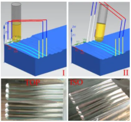
Fig. 5: The toolpath and machined workpiece. Table 1: Experimental cases for cutting force simulation Case Step no Cutting type Lead Tilt

I 1 Slotting 0 0

2,3 Half Immersion 0 0

II 1 Slotting 15 25

2,3 Half Immersion 15 25

5.1. Simulation of cutting forces

In 5-axis free form surface machining applications the cutter location points (CL) are distributed densely as the distance between consecutive CL points is governed by the geometrical tolerance. Thus, cutting force simulation is performed per p

number of CL points, which is selected depending on the case. The process simulation approach is verified through two cases. In the first case 3-axis ball end milling of a sculptured surface is considered, where the process is 5-axis milling of the same surface with tool inclination in the second case. The workpiece is Ti6Al4V and the cutting tool is 12 mm diameter carbide ball end mill with 2 cutting flutes and 30° helix angle, where the

spindle speed is 3000 rpm. The toolpath and machined workpiece are shown in Fig. 5, where the cutting parameters are listed in Table 1.

During the experiments, the cutting forces are measured using a rotary dynamometer. The x and y directions of the rotary dynamometer are not constant. Thus, the resultant transversal cutting force acting on the tool, i.e. Fxy, is simulated and compared with the measurements as shown in Fig. 6. The measurements and simulations agree well with reasonable accuracy. In Case 1, Fxy reaches up to 400 N during the engagement of the tool into the workpiece. Due to the wavy surface the cutting depth decreases and hence the cutting forces decreases to 100 N. Then, it increases up to 450 N at the end of the pass. In Case 2, Fxy reaches up to 450 N during the engagement and then decreases to 200 N in the middle of pass, then increases up to 500 N at the end of the pass.

(a) Case 1

(b) Case 2 Fig. 6: Experimental results.

5.2.Stability evaluation

The stability solution, summarized in section 4.2, is used to obtain stability diagrams to obtain the stable cutting depth for a range of spindle speeds. The aim of this study is to evaluate the stability of the process throughout the toolpath. Thus, the spindle speed and the engagement boundary is known at any CL point. The spindle speed is given in the CL file, and the engagement boundary is calculated using the distance field approach as given in Section 3. Thus, the stability limit is calculated for the known spindle speed and engagement boundary. Then, it is compared with the cutting depth at the corresponding cutter location point. This approach is applied on Case 1 and simulations are discussed.

The stability diagrams are generated for slotting and half immersion cases as plotted in Fig. 7a. It is seen that, at 3000 rpm, the stable cutting depth is around 1 mm and 1.25 mm for slotting and half immersion milling, respectively. The variation of the cutting depth along the tool axis is plotted in Fig. 7b, where the cutting depth varies between 0.6 mm and 2 mm. The process is expected to stable at the regions painted in green. Nonetheless, this needs further experimental verification.

(a) Stability limits (b) Variation of axial depth Fig. 7: The toolpath and machined workpiece. 6.Conclusions

In this paper, and integrated machining cycle simulation system is proposed, which consists of two main modules, i.e. generalized cutting force and process stability model and distance field based workpiece representation geometrical model. The system is able to simulate cutting forces and

(6)

stability for 5-axis ball end milling cycles. It is shown that distance field approach features very low computational time demands, close to real-time simulation. The cutting forces are modeled using orthogonal-to-oblique transformation based on a previously proposed model [10]. The cutting force simulations are compared with experimental results, where good agreement is observed. Process stability is simulated in frequency domain in order to detect stable and unstable cutting regions along a toolpath. Results obtained prove a very promising possibility of employing the distance field workpiece representation for real-time accurate simulations of cutting forces and stability predictions. However, simulations regarding process stability need further verification.

Acknowledgements

The authors gratefully acknowledge the support of ESPRC, The University of Manchester and The University of Sheffield under NNUMAN Programme with grant number EP/J021172/1. Support of the Competence Center - Manufacturing Technology project TE01020075 funded by the Technology Agency of the Czech Republic is also gratefully acknowledged.

References

[1] Altintas, Y., Kersting, P., Biermann, D., Budak, E., Denkena, B., Lazoglu, I. Virtual process systems for part machining operations, CIRP Annals – Manufacturing Technology; 2014, p.585-605.

[2] Budak E. Analytical methods for high performance milling-part I: forces, form error and tolerance integrity, Int. J of Machine Tools and Manufacture; 2006, p.1478, 2006.

[3] Budak E. Analytical Models for High Performance Milling. Part II: Process Dynamics and Stability, International Journal of Machine Tool & Manufacture; 2006, p.1489-1499.

[4] Lee P., Altintas, Y. Prediction of ball-end milling forces from orthogonal cutting data. Int. J. Machine Tools Manuf ;1996. p.1059–1072. [5] Armarego, E.J.A, Epp, C.J. An investigation of zero helix peripheral

up-milling, Int. J. of Machine Tool Design and Research; 1970. p.273-291. [6] Engin, S. and Altintas, Y. Mechanics and dynamics of general milling

cutters. Part I: helical end mills, Int. J. of Machine Tools & Manufacture; 2001. pp. 2213-2231.

[7] Engin, S. and Altıntaş, Y. Mechanics and dynamics of general milling cutters. Part II: inserted cutters, Int. J. of Machine Tools & Manufacture; 2001. pp. 2195-2212.

[8] Ozturk E, Budak E. Modeling of 5-axis milling processes, Machining Science and Technology; 2007. p.287-311.

[9] Kaymakci, M., Kilic, Z.M., Altintas, Y. Unified cutting force model for turning, boring, drilling and milling operations, Int. J. Mach. Tools Manuf; 2012. pp.34–45.

[10]Tunc L.T., Ozkirimli O.O., Budak E. Generalized cutting force model in multi-axis milling using a new engagement boundary determination approach. The Int. J of Advanced Manufacturing Technology; 2014. DOI: 10.1007/s00170-014-6453-8.

[11]Koenigsberger, F., Tlusty, J. Machine Tool Structures-Vol. I: Stability Against Chatter, Pergamon Press, Oxford; 1967.

[12]Opitz,H.,Bernardi,F. Investigation and calculation of the chatter behavior of lathes and mlling machines,Annals of the CIRP;1970. p.335-343. [13]Minis, I., Yanushevsky, T., Tembo, R., Hocken, R. Analysis of linear and

nonlinear chatter in milling, Annals of CIRP;1990, pp.459-462.

[14]Budak, E., Altintas, Y. Analytical prediction of chatter stability in milling. Part I-II; ASME Journal of Dynamic System Measurement and Control; 1998. pp.22-36.

[15]Altintas, Y., Shamoto, E., Lee, P., Budak, E. Analytical prediction of stability lobes in ball end milling, ASME J. Manuf Sci and Eng; 1999. pp596-592.

[16]Ozturk E., Budak E., Dynamics and stability of 5-axis ball end milling, J. of Manuf. Sci. and Eng.; 2010. 1-12.

[17]Campomanes, M. L. Kinematics and dynamics of milling with roughing endmills, Metal Cutting and High Speed Machining, Kluwer Academic/Plenum Publishers; 2002.

[18]Merdol, S.D.,Altintas, Y. Mechanics and dynamics of serrated cylindrical and tapered end mills, J. of Manuf Sci and Eng; 2004. p.217-236. [19]Dombovari, Z., Altintas, Y., Stephan G. The effect of serration on

mechanics and stability of milling cutters, International J of Machine Tools & Manufacture; 2010. pp.511-520.

[20]Slavicek, J., The effect of irregular tooth pitch on stability in milling, Proc 6th MTDR Conf; 1965 pp. 15–22.

[21]Altintas,Y.,Engin, S.,Budak, E.,Analytical stability prediction and design of variable pitch cutters, J of Manuf Sci and Eng; 1999. pp.173-178. [22]Van, H., T. Real-time shaded NC milling display. ACM SIGGRAPH

Computer Graphics, 20-4; 1986. p. 15 – 20

[23]Inui, M., Kakio, R. Fast visualization of NC milling result using graphics acceleration hardware. Proceedings 2000 ICRA. Millennium Conference. IEEE International Conference on Robotics and Automation. Symposia Proceedings;2000,Cat.No.00CH37065.DOI: 10.1109/robot.2000.845138. [24]Lavernhe, S., Quinsat, Y., Lartigue, C. Model for the prediction of 3D

surface topography in 5-axis milling. Int Journal of Advanced Manufacturing Technology, 51/9-12; 2010. p.912–915. DOI 10.1007/s00170-010-2686-3

[25]Sulitka, M., Vesely, J., Linkeova, I., Felkel, P. Normal based visualization of the virtually machined surface for capturing the impact of machine tool complex dynamic properties. Proceedings of the 9th International Conference on HIGH SPEED MACHINING; 2012, San Sebastian, 2012, p. 1-6. ISBN 978-84-932064-6-8

[26]Muller, H., Surmann, Tobias., Stautner, M., Albersmann, F., Weinert, K. Online sculpting and visualization of multi-dexel volumes. Proceedings of the 8th_{ACM symposium on Solid modeling and applications. 2003, SM'03.} DOI: 10.1145/781644.781646.

[27]Ren, Y., Lai-Yuen, S.K., Lee, Y.S. Virtual prototyping and manufacturing planning by using tri-dexel models and haptic force feedback. Virtual and Physical Prototyping, 1-3; 2006. p.3–18. DOI: 10.1080/17452750500283590

[28]Yagel, R., Cohen, D., Kaufman, A. Discrete ray tracing. IEEE Computer Graphics and Applications, 12-5; 1992. p.19–28 DOI 10.1109/38.156009 [29]Jang, D., Kwangsoo, K., Jungmin, J., Radzevich, S., Voxel-Based Virtual Multi-Axis Machining. The Int. J. of Adv. Manufacturing Technology, 16-10; 2000. p. 709-713. DOI: 10.4271/2006-01-0381.

[30]Ding, S., Mannan, M.A., Poo, A.N. Oriented bounding box and octree based global interference detection in 5-axis machining of free-form surfaces. Computer-Aided Design. 36-13; 2004. p. 1281-1294. DOI: 10.1016/S0010-4485(03)00109-X.

[31]PORTER-SOBIERAJ, Joanna a Maciej ŚWIECHOWSKI. Fast and accurate machined surface rendering using an octree Model. ICCVG 2010, LNCS 6375; 2010. p. 276-283.

[32]Jamriška, O., Havran, V. Interactive Ray Tracing of Distance Fields. Proceedings of The 14th Central European Seminar on Computer Graphics, Wien; 2010.

[33]Sullivan, A., Erdim, H., Perry, R., N., Frisken, S. F., High accuracy NC milling simulation using composite adaptively sampled distance fields. Computer-Aided Design 44, 2012, pp. 522 - 536.

[34]http://www.malinc.com/products/machpro/ [35]http://www.maxima.com.tr