University of California, Berkeley
U.C. Berkeley Division of Biostatistics Working Paper Series
Year Paper
Multiple Hypothesis Testing in Microarray
Experiments
Sandrine Dudoit
∗Juliet Popper Shaffer
†Jennifer C. Boldrick
‡∗Division of Biostatistics, University of California, Berkeley, [email protected] †Department of Statistics, University of California, Berkeley
‡Dept. of Microbiology & Immunology, Stanford University
This working paper is hosted by The Berkeley Electronic Press (bepress) and may not be commer-cially reproduced without the permission of the copyright holder.
http://biostats.bepress.com/ucbbiostat/paper110 Copyright c2002 by the authors.
Multiple Hypothesis Testing in Microarray
Experiments
Sandrine Dudoit, Juliet Popper Shaffer, and Jennifer C. Boldrick
Abstract
DNA microarrays are a new and promising biotechnology which allows the mon-itoring of expression levels in cells for thousands of genes simultaneously. An important and common question in microarray experiments is the identification of differentially expressed genes, i.e., genes whose expression levels are associated with a response or covariate of interest. The biological question of differential expression can be restated as a problem in multiple hypothesis testing: the simul-taneous test for each gene of the null hypothesis of no association between the expression levels and the responses or covariates. As a typical microarray ex-periment measures expression levels for thousands of genes simultaneously, large multiplicity problems are generated. This article discusses different approaches to multiple hypothesis testing in the context of microarray experiments and com-pares the procedures on microarray and simulated datasets.
1
Introduction
The burgeoning field of genomics has revived interest in multiple testing procedures by raising new methodological and computational challenges. For example, microarray experiments gener-ate large multiplicity problems in which thousands of hypotheses are tested simultaneously. DNA microarrays are a new and promising biotechnology which allows the monitoring of expression lev-els in cells for thousands of genes simultaneously. Microarrays are being applied increasingly in biological and medical research to address a wide range of problems, such as the classification of tumors or the study of host genomic responses to bacterial infections (Alizadeh et al. 2000, Alon et al. 1999, Boldrick et al. 2002, Golub et al. 1999, Perou et al. 1999, Pollack et al. 1999, Ross et al. 2000). An important and common question in microarray experiments is the identification of differentially expressed genes, i.e., genes whose expression levels are associated with a response or covariate of interest. The covariates could be either polytomous (e.g. treatment/control status, cell type, drug type) or continuous (e.g. dose of a drug, time), and the responses could be, for example, censored survival times or other clinical outcomes. The biological question of differential expression can be restated as a problem in multiple hypothesis testing: the simultaneous test for each gene of the null hypothesis of no association between the expression levels and the responses or covariates. As a typical microarray experiment measures expression levels for thousands of genes simultane-ously, large multiplicity problems are generated. In any testing situation, two types of errors can be committed: a false positive, or Type I error, is committed by declaring that a gene is differentially expressed when it isn’t, and a false negative, or Type II error, is committed when the test fails to identify a truly differentially expressed gene. When many hypotheses are tested and each test has a specified Type I error probability, the chance of committing some Type I errors increases, often sharply, with the number of hypotheses. In particular, ap–value of 0.01 for one gene among a list of several thousands will no longer correspond to a significant finding, as it is inevitable that such smallp–values will occur by chance when considering a large enough set of genes. Special problems arising from the multiplicity aspect include defining an appropriate Type I error rate and devising powerful multiple testing procedures which control this error rate and account for the joint distri-bution of the test statistics. A number of recent papers have addressed the question of multiple testing in microarray experiments (Dudoit et al. 2002, Efron et al. 2000, Golub et al. 1999, Kerr et al. 2000, Manduchi et al. 2000, Tusher et al. 2001, Westfall et al. 2001). However, the proposed solutions have not always been cast in the standard statistical framework.
This article discusses different approaches to multiple hypothesis testing in the context of microarray experiments and compares the procedures on microarray and simulated datasets. Section 2 reviews basic notions and approaches to multiple testing, and discusses the recent proposals of Efron et al. (2000), Golub et al. (1999), and Tusher et al. (2001) within this framework. The microarray datasets and simulation models which are used to evaluate the different multiple testing procedures are described in Section 3 and the results of the comparison study are presented in Section 4. Finally, Section 5 summarizes our findings and outlines open questions. Although the focus is on the identification of differentially expressed genes in microarray experiments, some of the methods described in this article are applicable to any large–scale multiple testing problem.
2
Methods
2.1 Multiple testing in microarray experiments
Consider a microarray experiment which produces expression data onm genes (or variables) forn
mRNA samples, and further suppose that a response or covariate of interest is recorded for each sample. Such data may arise, for example, from a study of gene expression in tumor biopsy speci-mens from leukemia patients (Golub et al. 1999): in this case, the response is the tumor type and the goal is to identify genes that are differentially expressed in the different types of tumors. The data for sampleiconsist of a response or covariateyi and a gene expression profilexi= (x1i, . . . , xmi), wherexji denotes the expression level of genejin samplei,i= 1, . . . , n,j = 1, . . . , m. The expres-sion levelsxjimight be either absolute (e.g. Affymetrix oligonucleotide chips (Lockhart et al. 1996)) or relative with respect to the expression levels of a suitably defined common reference sample (e.g.
Stanford two–color cDNA microarrays (Brown & Botstein 1999, DeRisi et al. 1997)). Note that the expression levels xji are in general highly processed data. The raw data in a microarray ex-periment consist of image files, and important preprocessing steps include image analysis of these scanned images and normalization (Yang, Buckley, Dudoit & Speed 2002, Yang et al. 2001, Yang, Dudoit, Luu, Lin, Peng, Ngai & Speed 2002). The gene expression data are conventionally stored in anm×nmatrixX= (xji), with rows corresponding to genes and columns to individual mRNA samples 1. In a typical experiment, the total number n of samples is anywhere between around ten and a few hundreds, and the number m of genes is several thousands. The gene expression levels,x, are continuous variables, while the response or covariate,y, could be either polytomous or continuous as described above. LetXj denote the random variable corresponding to the expression level for gene j and letY denote the response or covariate.
The biological question of differential expression can be restated as a problem in multiple hypothesis testing: the simultaneous test for each gene j of the null hypothesis Hj of no association between
Xj and Y. A standard approach to this problem consists of two aspects: (1) computing a test statisticTj for each gene j, and (2) applying a multiple testing procedure to determine which hy-potheses to reject while controlling a suitably defined Type I error rate (Dudoit et al. 2002, Efron et al. 2000, Golub et al. 1999, Kerr et al. 2000, Manduchi et al. 2000, Tusher et al. 2001, Westfall et al. 2001).
The univariate problem in (1) has been studied extensively in the statistical literature. In general, the appropriate test statistic will depend on the experimental design and the type of response or covariate. For example, for binary covariates one might consider at– or a Mann–Whitney statistic, for categorical responses one might use an F–statistic, and for survival data one might rely on the score statistic for the Cox proportional hazard model. We won’t discuss the choice of statistic any further here, except to say that for each gene j the null hypothesis Hj is tested based on a statistic Tj, where tj denotes a realization of the random variable Tj. To simplify matters, and unless specified otherwise, we further assume that the null Hj is rejected for large values of |Tj| (two–sided hypotheses). Question (2) is the subject of the present article. Although multiple testing is by no means a new subject in the statistical literature, microarray experiments present a new and challenging area of application for multiple testing procedures because of the sheer number of comparisons. In the remainder of this section, we review basic notions and approaches to
1Note that this gene expression data matrix is the transpose of the standard n×mdesign matrix. The m×n
representation was adopted in the microarray literature for display purposes, since for very largemand smallnit is easier to display anm×nmatrix than ann×mmatrix.
multiple testing, and discuss recent proposals for dealing with the multiplicity problem in microarray experiments.
2.2 Type I error rates
Set–up. Consider the problem of testing simultaneously m null hypotheses Hj, j = 1, . . . , m,
and denote by R the number of rejected hypotheses. In the frequentist setting, the situation can be summarized by the table below (Benjamini & Hochberg 1995). The specific m hypotheses are assumed to be known in advance, the numbers m0 and m1 = m−m0 of true and false null hypotheses are unknown parameters, R is an observable random variable, and S, T, U, and V
are unobservable random variables. In the microarray context, there is a null hypothesis Hj for each gene j and rejection of Hj corresponds to declaring that gene j is differentially expressed. In general, one would like to minimize the number V of false positives, or Type I errors, and the numberT of false negatives, orType II errors. The standard approach in a univariate setting is to prespecify an acceptable Type I error rateα and seek tests which minimize the Type II error rate,
i.e., maximizepower, within the class of tests with Type I error rateα.
# not rejected # rejected
# true null hypotheses U V m0
# non–true null hypotheses T S m1
m−R R m
Type I error rates. When testing a single hypothesis, H1, say, the probability of a Type I error,
i.e., of rejecting the null hypothesis when it is true, is usually controlled at some designated levelα. This can be achieved by choosing a critical value cα such that pr(|T1| ≥cα|H1) ≤α and rejecting H1 when |T1| ≥cα. A variety of generalizations to the multiple testing situation are possible; the Type I error rates described next are the most standard (Shaffer 1995).
• Per–comparison error rate (PCER). The PCER is defined as the expected value of (number
of Type I errors/number of hypotheses),i.e.,
P CER=E(V)/m.
• Per–family error rate (PFER). The PFER is defined as the expected number of Type I errors,
i.e.,
P F ER=E(V).
• Family–wise error rate (FWER). The FWER is defined as the probability of at least one
Type I error,i.e.,
• False discovery rate (FDR). The FDR of Benjamini & Hochberg (1995) is the expected pro-portion of Type I errors among the rejected hypotheses, i.e.,
F DR=E(Q), where by definition Q= ( V /R, ifR >0, 0, ifR= 0.
Strong vs. weak control. It is important to note that the expectations and probabilities above
areconditionalon which hypotheses are true. A fundamental, yet often ignored distinction, is that
between strong and weak control of the Type I error rate. Strong controlrefers to control of the Type I error rate under any combination of true and false hypotheses, i.e., any value of m0. In contrast,weak control refers to control of the Type I error rate only when all the null hypotheses are true, i.e., under the complete null hypothesis HC0 = ∩jm=1Hj with m0 = m. In other words, for the FWER, weak control means control ofpr(V ≥1|HC0), while strong control means control of maxΛ0⊆{1,...,m}pr(V ≥1 | ∩j∈Λ0Hj). In general, weak control without any other safeguards is unsatisfactory. In the microarray setting, where it is very unlikely that no genes are differentially expressed, it seems particularly important to have strong control of the Type I error rate. In the remainder of this article, unless specified otherwise, probabilities and expectations are com-puted under arbitrary combinations of true and false hypotheses, that is, under the null hypotheses
∩j∈Λ0Hj for some arbitrary subset Λ0⊆ {1, . . . , m}of size m0.
Power. Within the class of multiple testing procedures that control a given Type I error rate at an
acceptable levelα, one seeks procedures that maximize power, that is, minimize a suitably defined Type II error rate. As with Type I error rates, the concept of power can be generalized in various ways when moving from single to multiple hypothesis testing. Three common definitions of power are: (i) the probability of rejecting at least one false null hypothesis,pr(S≥1) =pr(T ≤m1−1); (ii) the average probability of rejecting the false null hypotheses,E(S)/m1, or average power; and (iii) the probability of rejecting all false null hypotheses, pr(S =m1) =pr(T = 0) (Shaffer 1995). When the family of tests consists of pairwise mean comparisons, these quantities have been called any–pair power, per–pair power, and all–pairs power (Ramsey 1978). In a spirit analogous to the FDR, one could also define power asE(S/R|R >0)pr(R >0) =pr(R >0)−F DR; whenm=m1, this is the any–pair power pr(S ≥1). One should note again that probabilities are conditional on which null hypotheses are true and which are false.
Comparison of Type I error rates. In general, for a given multiple testing procedure,P CER≤
F W ER ≤ P F ER. Thus, for a fixed criterion α for controlling the Type I error rates, the order reverses for the number of rejections R: procedures controlling the PFER are generally more conservative than those controlling either the FWER or the PCER, and procedures controlling the FWER are more conservative than those controlling the PCER. To illustrate the properties of the different Type I error rates, suppose each hypothesis Hj is tested individually at level αj and the decision to reject or not reject this hypothesis is based solely on that test. Under the complete null hypothesis, the PCER is simply the average of theαj and the PFER is the sum of theαj. In contrast, the FWER is a function not of the test sizesαj alone, but involves the jointdistribution of the test statisticsTj
The FDR also depends on the joint distribution of the test statistics and, for a fixed procedure,
F DR≤F W ER, withF DR=F W ERunder the complete null. The classical approach to multi-ple testing calls for strong control of the FWER (e.g. Bonferroni procedure). The recent proposal of Benjamini & Hochberg (1995) controls the FWER in the weak sense and can be less conserva-tive than FWER otherwise. Procedures controlling the PCER are generally less conservaconserva-tive than those controlling either the FDR or FWER, but tend to ignore the multiplicity problem altogether. The following simple example describes the behavior of the various Type I error rates as the total number of hypotheses mand the proportion of true hypothesesm0/mvary.
A simple example. Consider random Gaussian m–vectors with mean µ = (µ1, . . . , µm) and
identity covariance matrixIm. Suppose we wish to test simultaneously them null hypotheses Hj :
µj = 0 against the two–sided alternatives H0j :µj 6= 0. Given a random sample ofn m–vectors from this distribution, a simple multiple testing procedure would be to reject Hjif|X¯j| ≥zα/2/
√
n, where ¯
Xjis the average of thejth coordinate for then m–vectors,zα/2is such that Φ(zα/2) = 1−α/2, and Φ(·) is the standard normal cumulative distribution function. Let Rj=I(|X¯j| ≥zα/2/
√
n), where
I(·) is the indicator function, equaling 1 if the condition in parentheses is true, and 0 otherwise, and assume without loss of generality that the m0 true null hypotheses are H1, . . . ,Hm0. Then
V = Pmj=10 Rj, R =
Pm
j=1Rj, and analytical formulae for the Type I error rates can easily be derived as P F ER = m0 X j=1 γj, P CER = m0 X j=1 γj/m, F W ER = 1− m0 Y j=1 (1−γj), F DR = 1 X r1=0 . . . 1 X rm=0 Pm0 j=1rj Pm j=1rj m Y j=1 γjrj(1−γj)1−rj,
with the FDR convention that 0/0 = 0 andγj=E(Rj) = 1−Φ(zα/2−µj√n) + Φ(−zα/2−µj√n) denoting the chance of rejecting hypothesis Hj. In our simple example, γj =α forj = 1, . . . , m0, and if we further assume thatµj =d/√n forj =m0+ 1, . . . , m, then the expressions for the error rates simplify to P F ER = m0α, P CER = m0α/m, F W ER = 1−(1−α)m0, F DR = m1 X s=0 m0 X v=1 v v+s m0 v αv(1−α)m0−v m1 s βs(1−β)m1−s,
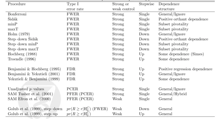
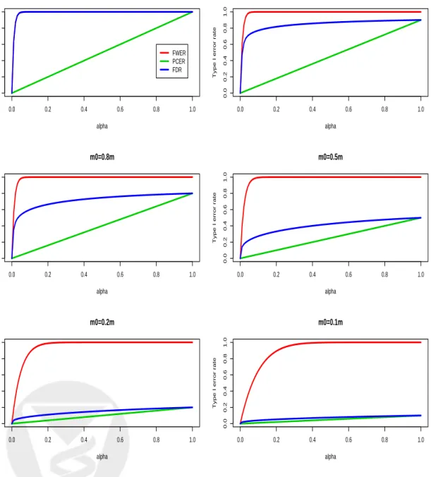
where β = 1−Φ(zα/2 −d) + Φ(−zα/2−d). Note that unlike the PFER, FWER, or PCER, the FDR depends on the distribution of the test statistics for the false null hypotheses through the random variableS. In general, the FDR is thus more complicated to compute. Figure 1 displays plots of the FWER, PCER, and FDR vs. the number of hypotheses m, for different proportions
m0/m= 1,0.9,0.8,0.5,0.2,0.1 of true null hypotheses, and for α = 0.05 and d= 1. In general, the FWER and PFER increase sharply with the number of hypothesesm, while the PCER remains constant (the PFER is not shown on the figure because it is on a different scale). Under the complete null m = m0, the FDR is equal to the FWER and both increase sharply with m. However, as the proportion of true null hypotheses m0/m decreases, the FDR remains relatively stable as a function of m and approaches the PCER. Figure 2 displays plots of the FWER, PCER, and FDR
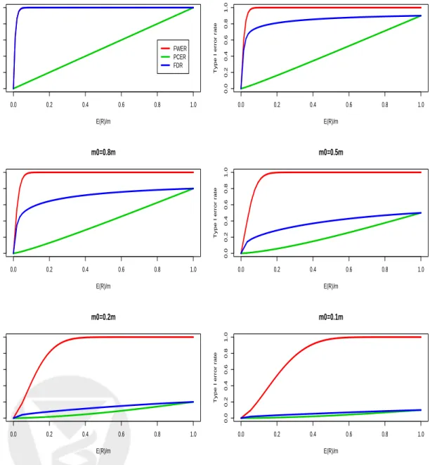
vs. individual test size α, for different proportionsm0/mof true null hypotheses, and form= 100 andd= 1. The FWER is generally much larger than the PCER, the largest difference being under the complete nullm=m0. As the proportion of true null hypotheses decreases, the FDR becomes closer to the PCER. Similar behavior of the error rates is displayed in Figure 3, which plots Type I error rates vs. expected proportion of rejected hypotheses E(R)/m, for different proportions
m0/mof true null hypotheses, and for m = 100 andd= 1. These plots can be used to compare the different Type I error rates one would expect for a given number of rejected hypotheses.
2.3 Adjusted p–values
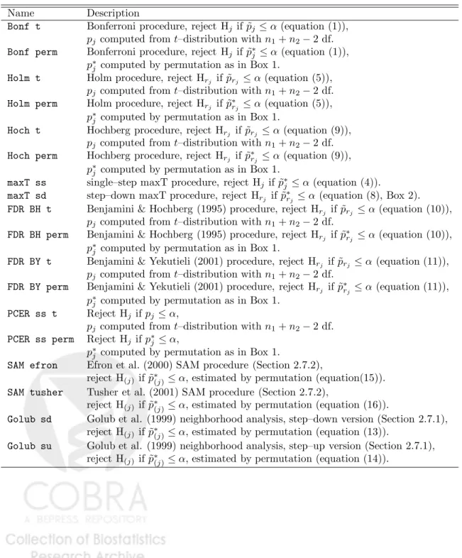
Unadjusted p–values. Consider first a single hypothesis H1, say, and a family of tests of H1,
with level–αnested rejection regions Sα such that: (a)pr(T1 ∈Sα|H1) =α for allα ∈[0,1] which are achievable under the distribution of T1, and (b) Sα0 = ∩α≥α0Sα for all α and α0 for which these regions are defined in (a). Rather than simply reporting rejection or not of the hypothesis, a
p–value connected with the test can be defined as p1 = inf{α :t1 ∈ Sα} (adapted from Lehmann
(1986), p. 170, to include discrete test statistics). Thep–value can be thought of as the level of the test at which the hypothesis H1 would just be rejected. The smaller the p–value p1, the stronger the evidence against the null hypothesis H1. Rejecting H1 when p1 ≤ α provides control of the Type I error rate at levelα. In our context, thep–value can also be restated as the probability of observing a test statistic as extreme or more extreme in the direction of rejection as the observed one, that is,p1 =pr(|T1| ≥ |t1||H1). Extending this concept to the multiple testing situation leads to the very useful notion of adjusted p–value.
Adjusted p–values. Let tj and pj =pr(|Tj| ≥ |tj||Hj) denote respectively the test statistic and
p–value for hypothesis Hj (genej), j= 1, . . . , m. Just as in the single hypothesis case, a multiple testing procedure may be defined in terms of critical values for the test statistics or p–values of individual hypotheses: e.g. reject Hj if |tj| ≥cj or if pj ≤αj, where the critical values cj and αj are chosen to control a given Type I error rate (FWER, PCER, PFER, or FDR) at a prespecified levelα. Alternatively, the multiple testing procedure may be defined in terms of adjustedp–values. Given any test procedure, the adjusted p–value corresponding to the test of a single hypothesis Hj can be defined as the level of the entire test procedure at which Hj would just be rejected, given the values of all test statistics involved (Hommel & Bernhard 1999, Shaffer 1995, Westfall & Young 1993, Wright 1992, Yekutieli & Benjamini 1999). If interest is in controlling the FWER, the FWER adjustedp–value for hypothesis Hj is
˜
pj = inf{α∈[0,1] : Hj is rejected at F W ER=α}.
The corresponding random variables for unadjusted (or raw) and adjusted p–values are denoted by Pj and ˜Pj, respectively. Hypothesis Hj is then rejected, i.e., gene j is declared differentially expressed, at FWERα if ˜pj ≤α. Adjusted p–values for other Type I error rates are defined simi-larly, that is, for the FDR, ˜pj = inf{α : Hj is rejected at F DR=α}(Yekutieli & Benjamini 1999). As in the single hypothesis case, an advantage of reporting adjusted p–values, as opposed to only
rejection or not of the hypotheses, is that the level of the test does not need to be determined in advance. Some multiple testing procedures are also most conveniently described in terms of their adjustedp–values and these can in turn be easily determined using resampling methods (Westfall & Young 1993).
Stepwise procedures. One usually distinguishes among three types of multiple testing
pro-cedures: single–step, step–down, and step–up procedures. In single–step procedures, equivalent multiplicity adjustments are performed for all hypotheses, regardless of the ordering of the test statistics or unadjusted p–values, that is, each hypothesis is evaluated using a critical value that is independent of the results of tests of other hypotheses. Improvement in power, while preserving Type I error rate control, may be achieved bystepwise procedures, in which rejection of a particular hypothesis is based not only on the total number of hypotheses, but also on the outcome of the tests of other hypotheses. Instep–downprocedures, the hypotheses corresponding to themostsignificant test statistics (i.e., smallest unadjusted p–values or largest absolute test statistics) are considered successively, with further tests depending on the outcomes of earlier ones. As soon as one hypoth-esis is accepted, all remaining hypotheses are accepted. In contrast, for step–up procedures, the hypotheses corresponding to the least significant test statistics are considered successively, again with further tests depending on the outcomes of earlier ones. As soon as one hypothesis is re-jected, all remaining hypotheses are rejected. The next section discusses single–step and stepwise procedures for control of the FWER.
2.4 Control of the family–wise error rate
2.4.1 Single–step procedures
For strong control of the FWER at level α, the Bonferroni procedure, perhaps the best known in multiple testing, rejects any hypothesis Hj with p–value less than or equal to α/m. The corre-spondingsingle–step Bonferroni adjusted p–values are thus given by
˜
pj = min mpj,1
. (1)
Control of the FWER in the strong sense follows from Boole’s inequality. Assume without loss of generality that the true null hypotheses are Hj, for j = 1, . . . , m0, then, for Pj having a U[0,1] distribution under Hj F W ER=pr(V ≥1) =pr m0 [ j=1 {P˜j ≤α}≤ m0 X j=1 pr P˜j ≤α ≤ m0 X j=1 pr Pj ≤α/m =m0α/m.
Closely related to the Bonferroni procedure is the ˇSid´ak procedure which is exact under the complete null for protecting the FWER when the unadjusted p–values are independently distributed as
U[0,1]. The single–step Sˇid´ak adjustedp–valuesare given by ˜
pj = 1−(1−pj)m. (2)
However, in many situations, the test statistics and hence thep–values are correlated. This is the case in microarray experiments, where groups of genes tend to have highly correlated expression levels due, for example, to co–regulation. Westfall & Young (1993) propose adjusted p–values for
less conservative multiple testing procedures which take into account the dependence structure among test statistics. Thesingle–step minP adjusted p–values are defined by
˜
pj =pr min
1≤l≤mPl ≤pj |H C
0, (3)
where HC0 denotes the complete null hypothesis and Pl the random variable for the unadjusted
p–value of the lth hypothesis. Alternatively, one may consider procedures based on thesingle–step
maxT adjusted p–values which are defined in terms of the test statisticsTj themselves
˜
pj =pr max
1≤l≤m|Tl| ≥ |tj||H
C
0. (4)
The following points should be noted regarding these four procedures.
1. If the unadjustedp–values (P1, . . . , Pm) are independent andPj has aU[0,1] distribution under Hj, the minP adjustedp–values are the same as the ˇSid´ak adjustedp–values.
2. The ˇSid´ak procedure does not guarantee control of the FWER for arbitrary distributions of the test statistics, however, it controls the FWER for test statistics that satisfy an inequality known as ˇSid´ak’s inequality: pr(|T1| ≤ c1, . . . ,|Tm| ≤ cm) ≥
Qm
j=1pr(|Tj| ≤ cj). This inequality, also known as the positive orthant dependence property, was initially derived by Dunn (1958) for (T1, . . . , Tm) having a multivariate normal distribution with mean zero and certain types of covari-ance matrix. ˇSid´ak (1967) extended the result to arbitrary covariance matrices, and Jogdeo (1977) showed that the inequality holds for a larger class of distributions, including the multivariate t– and F–distributions. When the ˇSid´ak inequality holds, the minP adjusted p–values are less than or equal to the ˇSid´ak adjustedp–values.
3. Computing the quantities in (3) using the upper bound provided by Boole’s inequality yields the Bonferronip–values, for unadjustedp–values Pl∼U[0,1] marginally under Hl.
In other words, procedures based on the minP adjusted p–values are less conservative than the Bonferroni or ˇSid´ak (under the ˇSid´ak inequality) procedures. In the case of independent test statis-tics, the ˇSid´ak and minP adjustments are equivalent as discussed in item 1, above.
4. Procedures based on the maxT and minP adjustedp–values control the FWER weakly under all conditions. Strong control of the FWER also holds under the assumption of subset pivotality (Westfall & Young 1993, p. 42). The distribution of unadjusted p–values (P1, . . . , Pm) is said to have thesubset pivotality property if the joint distribution of the sub–vector{Pj :j ∈Λ0}is identi-cal under the restrictions∩j∈Λ0Hj and HC0 =∩mj=1Hj, for all subsets Λ0 of{1, . . . , m}. The subset pivotality condition is important because it ensures that procedures based on adjusted p–values computed under the complete null provide strong control of the FWER. A practical consequence of this property is that resampling for computing adjustedp–values may be done conveniently under the complete null rather than the partial null hypotheses. Without subset pivotality, multiplicity adjustment is more complex.
5. The maxT p–values are easier to compute than the minP p–values and are equal to the minP
p–values when the test statisticsTj are identically distributed. However, the two procedures gener-ally produce different adjustedp–values, and considerations of balance, power, and computational
feasibility should dictate the choice between the two approaches. In the case of non–identically distributed test statisticsTj (e.g. t–statistics with different degrees of freedom), not all tests con-tribute equally to the maxT adjustedp–values and this can lead to unbalanced adjustments (Beran 1988, Westfall & Young 1993, p. 50). When adjustedp–values are estimated by permutation (Sec-tion 2.6) and a large number of hypotheses are tested, procedures based on the minPp–values tend to be more sensitive to the number of permutations and more conservative than those based on the maxT p–values. Also, the minP p–values require more computations than the maxTp–values, because the unadjusted p–values must be computed before considering the distribution of their successive minima (Ge & Dudoit 2002).
2.4.2 Step–down procedures
While single–step procedures are simple to implement, they tend to be conservative for control of the FWER. Improvement in power, while preserving strong control of the FWER, may be achieved by step–down procedures. Below are the step–down analogs, in terms of their adjustedp–values, of the four procedures described in the previous section. Letpr1 ≤pr2 ≤...≤prmdenote theobserved
ordered unadjusted p–values, and Hr1,Hr2, . . . ,Hrm the corresponding null hypotheses. For control
of the FWER at levelα, the Holm (1979) procedure proceeds as follows. Define
j∗ = min n j :prj > α m−j+ 1 o
and reject hypotheses Hrj, for j = 1, . . . , j∗−1. If no such j∗ exists, reject all hypotheses. The
step–down Holm adjustedp–values are thus given by
˜ prj = maxk=1,...,j n min (m−k+ 1)prk,1 o . (5)
Holm’s procedure is less conservative than the standard Bonferroni procedure which would multiply thep–values bymat each step. Note that taking successive maxima of the quantities min (m−k+ 1)prk,1
enforces monotonicity of the adjusted p–values. That is, ˜pr1 ≤ p˜r2 ≤... ≤p˜rm, and one
can only reject a particular hypothesis provided all hypotheses with smaller unadjusted p–values were rejected beforehand. Similarly, thestep–down Sˇid´ak adjusted p–values are defined as
˜ prj = max k=1,...,j n 1−(1−prk)(m−k+1) o . (6)
The Westfall & Young (1993)step–down minP adjusted p–values are defined by ˜ prj = max k=1,...,j n pr min l∈{rk,...,rm} Pl≤prk |HC0 o , (7)
and the step–down maxT adjusted p–values are defined by ˜ prj = max k=1,...,j n pr max l∈{rk,...,rm}|Tl| ≥ |trk| |H C 0o, (8)
where |tr1| ≥ |tr2| ≥ ... ≥ |trm| denote the observed ordered test statistics. Note that computing the quantities in (7) under the assumption thatPl ∼U[0,1] and using the upper bound provided by Boole’s inequality yields Holm’sp–values. Procedures based on the step–down minP adjusted
p–values are thus less conservative than Holm’s procedure. For a proof of the strong control of the FWER for the maxT and minP procedures the reader is referred to Westfall & Young (1993, Section 2.8). Step–down procedures such as the Holm procedure may be further improved by taking into account logically related hypotheses as described in Shaffer (1986).
2.4.3 Step–up procedures
In contrast to step–down procedures, step–up procedures begin with the least significantp–value,
prm, and are usually based on the following probability result of Simes (1986). Under the complete
null hypothesis HC0 and for independent test statistics, the ordered unadjusted p–values P(1) ≤ P(2) ≤...≤P(m) satisfy
pr P(j)> αj/m, ∀ j= 1, . . . , m|HC0
≥1−α,
with equality in the continuous case. This inequality is known as theSimes inequality. In important cases of dependent test statistics, Simes showed that the probability was larger than 1−α, however this does not hold generally for all joint distributions.
The Hochberg (1988) procedure, based on the Simes inequality, can be viewed as a step–up modifi-cation of Holm’s step–down procedure, since the orderedp–values are compared to the same critical values in both procedures. For control of the FWER at level α, define
j∗= max n j:prj ≤ α m−j+ 1 o
and reject hypotheses Hrj, forj = 1, . . . , j∗. If no such j∗exists, reject no hypothesis. Thestep–up
Hochberg adjusted p–values are thus given by
˜ prj = min k=j,...,m n min (m−k+ 1)prk,1 o . (9)
Related procedures include those of Hommel (1988) and Rom (1990). Step–up procedures have often been found to be more powerful than their step–down counterparts; however, it is important to keep in mind that all procedures based on the Simes inequality rely on the assumption that the result proved under independence yields a conservative procedure for dependent tests. More research is needed to determine circumstances in which such methods are applicable, and in particular, whether they are applicable for the types of correlation structures encountered in microarray experiments. Troendle (1996) proposed a permutation–based step–up multiple testing procedure which takes into account the dependence structure among the test statistics and is related to the Westfall & Young (1993) step–down maxT procedure.
2.5 Control of the false discovery rate
A different approach to multiple testing was proposed in 1995 by Benjamini & Hochberg. These authors argue that, in many situations, control of the FWER can lead to unduly conservative pro-cedures and one may be prepared to tolerate some Type I errors, provided their number is small in comparison to the number of rejected hypotheses. These considerations led to a less conservative approach which calls for controlling the expected proportion of Type I errors among the rejected hypotheses – thefalse discovery rate, FDR. More specifically, the FDR is defined asF DR=E(Q), where Q = V /R if R > 0, and 0 if R = 0, i.e., F DR = E(V /R | R > 0)pr(R > 0). Under the complete null, given the definition of 0/0 = 0 when R = 0, the FDR is equal to the FWER; procedures controlling the FDR thus also control the FWER in the weak sense. Note that earlier references to the FDR can be found in Seeger (1968) and Sori´c (1989).
Benjamini & Hochberg (1995) derived the following step–up procedure for (strong) control of the FDR for independent test statistics. Let pr1 ≤ pr2 ≤ ... ≤ prm denote the observed ordered
unadjustedp–values. For control of the FDR at levelα define
j∗= max n j :prj ≤ j mα o
and reject hypotheses Hrj, forj= 1, . . . , j∗. If no suchj∗exists, reject no hypothesis.
Correspond-ing adjustedp–values are
˜ prj =k=minj,...,m n min m k prk,1 o . (10)
Benjamini & Yekutieli (2001) proved that this procedure controls the FDR under certain depen-dence structures (positive regression dependency). They also proposed a simple conservative modi-fication of the procedure which controls the false discovery rate for arbitrary dependence structures. For control of the FDR at levelα, define
j∗= max n j :prj ≤ j mPmj=11/jα o
and reject hypotheses Hrj, forj= 1, . . . , j∗. If no suchj∗exists, reject no hypothesis. Correspond-ing adjustedp–values are
˜ prj =k=minj,...,m n min mPm j=11/j k prk,1 o . (11)
For a large number m of hypotheses, the penalty in this conservative procedure is about logm, as compared to the Benjamini & Hochberg (1995) procedure. Note that the Benjamini & Hochberg procedure can also be conservative, even in the independence case, as it was shown that for this step–up procedureE(Q)≤ m0
mα≤α . Until recently, most FDR controlling procedures were either designed for independent test statistics or did not make use of the dependency structure among the test statistics. In the spirit of the Westfall & Young (1993) resampling procedures for FWER control, Yekutieli & Benjamini (1999) proposed new FDR controlling procedures which use resam-pling based adjustedp–values to incorporate certain types of dependency structures among the test statistics (the procedures assume among other things that the unadjustedp–values for the true null hypotheses are independent of thep–values for the false null hypotheses).
In the microarray setting, where thousands of comparisons are performed simultaneously and a fairly large number of genes are expected to be differentially expressed, FDR controlling procedures present a promising alternative to more conservative FWER approaches. In this context, one may be willing to bear a few false positives as long as their number is small in comparison to the number of rejected hypotheses. The problematic definition of 0/0 = 0 is also not as important in this case.
2.6 Resampling
In many situations, the joint (and marginal) distribution of the test statistics is unknown. Re-sampling methods (bootstrap or permutation) can be used to estimate unadjusted and adjusted
p–values while avoiding parametric assumptions about the joint distribution of the test statistics. In the microarray setting, the joint distribution under the complete null hypothesis of the test statistics (T1, . . . , Tm) can be estimated by permuting the columns of the gene expression data matrix X. Permuting entire columns of this matrix creates a situation in which the response or
covariate Y is independent of the gene expression levels, while attempting to preserve the cor-relation structure and distributional characteristics of the gene expression levels. Depending on the sample size n, it may be infeasible to consider all possible permutations, and in such a case a random subset of B permutations (including the observed) may be considered. The manner in which the responses/covariates are permuted depends on the experimental design, for example, for a two–factor design, one should permute the levels of the factor of interest within the levels of the other factor (see Scheff´e (1959), Section 9.3, and Section 3.2.2 for an example).
Box 1. Permutation algorithm for unadjusted p–values.
For the bth permutation,b= 1, . . . , B
1. Permute the ncolumns of the data matrixX.
2. Compute test statisticst1,b, . . . , tm,b for each hypothesis.
The permutation distribution of the test statisticTj for hypothesis Hj,j= 1, . . . , m, is given by the empirical distribution of tj,1, . . . , tj,B. For two–sided alternative hypotheses, the permutationp–value for hypothesis Hj is
p∗j =
PB
b=1I |tj,b| ≥ |tj|
B ,
where I(·) is the indicator function, equaling 1 if the condition in parentheses is true, and 0 otherwise.
Permutation adjusted p–values for the Bonferroni, ˇSid´ak, Holm, and Hochberg procedures can be obtained by replacingpj byp∗j in equations (1), (2), (5), (6), and (9). The permutation unadjusted
p–values can also be used for the FDR controlling procedures described in Section 2.5. For the step–down maxT adjusted p–values of Westfall & Young (1993), the null distribution of successive maxima maxl∈{rj,...,rm}|Tl|of the test statistics needs to be estimated (the single–step case is simpler and omitted here as we only need the distribution of the maximum maxl∈{r1,...,rm}|Tl|).
Box 2. Permutation algorithm for step–down maxT adjusted p–values – based on Algorithms 2.8 and 4.1 in Westfall & Young (1993).
For the bth permutation,b= 1, . . . , B
1. Permute the ncolumns of the data matrixX.
2. Compute test statisticst1,b, . . . , tm,b for each hypothesis. 3. Next, compute successive maxima of the test statistics
um,b = |trm,b| uj,b = max uj+1,b,|trj,b| forj=m−1, . . . ,1,
whererj are such that|tr1| ≥ |tr2| ≥...≥ |trm|for theoriginal data.
The adjusted p–values are estimated by
˜ p∗rj = PB b=1I uj,b≥ |trj| B ,
with the monotonicity constraints enforced by setting ˜
p∗r1 ← p˜r∗1, p˜∗rj ←max ˜p∗rj,p˜r∗j−1 forj= 2, . . . , m.
The reader is referred to Ge & Dudoit (2002) for a fast permutation algorithm for estimating minP adjustedp–values.
2.7 Recent proposals for microarray experiments
Efron et al. (2000), Golub et al. (1999), and Tusher et al. (2001) have recently proposed resampling algorithms for multiple testing in microarray experiments. However, these procedures were not presented within the standard statistical framework for multiple testing. In particular, the Type I error rates considered were rather loosely defined, thus making it difficult to assess the properties of the multiple testing procedures. These recent proposals are reviewed next, within the framework introduced in Sections 2.2 and 2.3.
2.7.1 Neighborhood analysis of Golub et al.
Golub et al. (1999) were interested in identifying genes that are differentially expressed in pa-tients with two type of leukemias, acute lymphoblastic leukemia (ALL, class 1) and acute myeloid leukemia (AML, class 2) (the study is described in greater detail in Section 3.2.3). In their so–called
neighborhood analysis, the authors compute a test statistictj for each gene (P(g, c) in their paper)
tj = ¯
x1j−x¯2j
s1j+s2j
,
where ¯xkj and skj denote respectively the average and standard deviation of the expression levels of genejin the classk= 1,2 samples. This statistic is based on anad hocdefinition of correlation, and resembles at–statistic with an unusual standard error calculation (note 16 in Golub et al.). It
is not pivotal,i.e., its null distribution depends on parameters of the distribution which generated the data, and a standard two–samplet–statistic should be preferred (note that this definition of pivotality is different from subset pivotality in Section 2.4). Statistics such astj have been used in meta–analysis to measure effect sizes (National Reading Panel 1999).
Golub et al. use the term “neighborhood” to refer to sets of genes with test statistics Tj greater in absolute value than a given critical value c, that is, sets of rejected hypotheses {j :Tj ≥c} or
{j : Tj ≤ −c} (these sets are denoted by N1(c, r) and N2(c, r) in note 16 of Golub et al.). The ALL/AML labels were permuted B = 400 times to estimate the complete null distribution of the numbersR(c) =V(c) =Pjm=1I(Tj ≥c) of false positives for different critical valuesc(similarly for the other tail, withTj ≤ −c). Figure 2 in Golub et al. contains plots of the observedR(c) =r(c) and permutation quantiles ofR(c) against critical values cfor one–sided tests 2. A critical value c
is then chosen so that the chance of exceeding the observed r(c) under the complete null is equal to a prespecified level α, that is,
G(c) =pr R(c)≥r(c)|HC0=α. (12)
Golub et al. provide no further guidelines for selecting the critical valuecor discussion of the Type I error control of their procedure. Like some PFER, PCER, or FWER controlling procedures, the neighborhood analysis considers the complete null distribution of the number of Type I errors
V(c) = R(c), however, instead of controllingE(V(c)), E(V(c))/m, or pr(V(c) ≥ 1), it seeks to control a different quantity, pr(R(c) ≥ r(c)|HC0), which can be thought of as a p–value under HC0 for the number of rejected hypotheses R(c) and is thus a random variable. For simplicity, consider continuous test statistics and two–sided hypotheses. Then, conditional on the observed ordered absolute test statistics, |t|(1) ≥ . . . ≥ |t|(m), the function G(c) is left–continuous, with discontinuities at|t|(j),j= 1, . . . , m, that is,
G(c) = pr R(c)≥m|HC0 pr R(c)≥j |HC0 pr R(c)≥0|HC0 = pr |T|(m)≥c|HC0 , ifc≤ |t|(m), pr |T|(j)≥c|HC0 , if|t|(j+1) < c≤ |t|(j), 1≤j≤m−1, 1, if|t|(1)< c.
Here, |T|(j) denote the ordered absolute test statistics, |T|(1) ≥ . . . ≥ |T|(m), and, in principle, different realizations of |T|(j) could correspond to different hypotheses. AlthoughG(c) is decreas-ing in c within intervals (|t|(j+1),|t|(j)], it is not in general decreasing overall, and there may be several values of c with G(c) = α. Hence, one must decide on an appropriate procedure for se-lecting the critical valuec. Two natural choices are given by stepwise procedures, as described next.
Step–down procedure. A step–down procedure would be to letc=|t|(j∗−1), where
j∗ = min n j:G(|t|(j))> α o = min n j :pr |T|(j)≥ |t|(j)|HC0 > α o ,
and reject hypotheses H(j), for j = 1, . . . , j∗−1. If no such j∗ exists, reject all hypotheses. The corresponding adjustedp–values are
˜ p(j)= max k=1,...,j n pr |T|(k)≥ |t|(k)|HC0 o . (13)
2We are aware that our notation can lead to confusion when compared with that of Golub et al. We chose to
follow the notation of Sections 2.2 and 2.3 to allow easy comparison with other multiple testing procedures described in the present article. For comparison with Golub et al. note that we use Tj to denoteP(g, c),cto denote r, and
Hence, the step–down adjustedp–values for the neighborhood analysis of Golub et al. are based on thep–valuespr |T|(j)≥ |t|(j)|HC
0
for the order statistics. Note that, unlike the Westfall & Young maxT procedure, where the adjustedp–values are based on pr maxl∈{rj,...,rm}|Tl| ≥ |trj| |HC0
for
thefixed ordering{rj} of the observed test statistics, the maxima in equation (13) could be taken
over different sets of hypotheses for different realizations of Tj. Because of this difference, it is unlikely that the step–down version of neighborhood analysis provides strong control of any Type I error rate, as the subset pivotality condition is not satisfied. A straightforward argument shows that the step–down procedure does, however, control the FWER weakly.
Step–up procedure. The corresponding step–up procedure would be to let c=|t|(j∗), where
j∗= max n j:G(|t|(j))≤α o = max n j:pr |T|(j)≥ |t|(j)|HC0≤α o ,
and reject hypotheses H(j), for j = 1, . . . , j∗. If no such j∗ exists, reject no hypothesis. The corresponding adjustedp–values are
˜ p(j)= min k=j,...,m n pr |T|(k)≥ |t|(k)|HC0 o . (14)
Again, it is unlikely that this procedure provides strong control of any Type I error rate, as the sub-set pivotality condition is not met. Furthermore, because of the step–up nature of the procedure and the non–monotonicity of the functionG(c), the FWER is not even controlled weakly. In this step– up procedure, hypothesis H(j) is rejected at nominal level α whenever pr |T|(k)≥ |t|(k) |HC0 ≤α
for somek≥j, thus each hypothesis is given several chances at rejection.
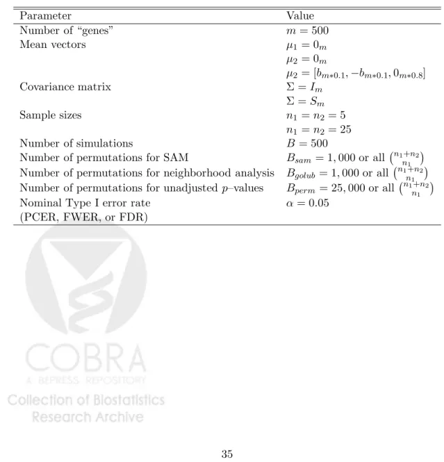
Figures 4 and 5 display plots of the observed number of rejected hypothesesr(c) and 95th permu-tation quantile of R(c) against the critical value c for data simulated from a model described in Table 3. Also shown are plots of the “Type I error rate” G(c) vs. c. These figures illustrate the non–monotonicity of G(c) and the possibility of having several values of c with G(c) = α. The plots of the step–down and step–up adjusted p–values demonstrate the importance of selecting the proper cin the case of several “crossings” of the observedr(c) with quantiles of R(c). For a fixed criterion α = 0.05, the step–up procedure starts from the left and looks for the first time G(c) dips below α = 0.05, while the step–down procedures starts from the right and looks for the first time G(c) rises above α = 0.05. When G(c) is monotone in c, the two procedures should yield the same results, otherwise, the step–up procedure generally produces a larger number of rejected hypotheses, but does not provide weak control of the FWER.
As a final remark, note that the number of permutations B = 400 used in Golub et al. (1999) is probably not large enough for reporting 99th quantiles in Figure 2. A better plot for Figure 2 of Golub et al. might be of the error rate G(c) = pr(R(c) ≥r(c) |HC0) vs. the critical values c, as this does not require a prespecified level α.
2.7.2 Significance Analysis of Microarrays (SAM) of Efron et al. and Tusher et al.
We consider two variants of the Significance Analysis of Microarrays or SAM multiple testing procedure, the original version in Efron et al. (2000) and the more recent Tusher et al. (2001) and Chu et al. (2000) version. Note that these manuscripts also address the question of choosing appropriate test statistics for different types of responses and covariates. Here, we focus only on
the proposed methods for dealing with the multiplicity problem and assume that a suitable test statistic is computed for each gene. The two SAM procedures are described next.
1. Compute a test statistic tj for each gene j and define order statistics t(j) such that t(1) ≥
t(2)≥. . .≥t(m) 3.
2. PerformB permutations of the responses/covariatesy1, . . . , yn. For each permutationb com-pute the test statisticstj,b and the corresponding order statisticst(1),b ≥t(2),b≥. . .≥t(m),b. Note that t(j),b may correspond to a different gene thant(j).
3. From theB permutations, estimate the expected value (under the complete null) of the order statistics by ¯t(j)= (1/B)
P
bt(j),b.
4. Form a Quantile–Quantile plot (so–called “SAM plot”) of the observedt(j) vs. the expected ¯
t(j).
5. – Efron et al. For a fixed threshold ∆, genes with|t(j)−t¯(j)| ≥∆ are declared “significant”,
i.e., the corresponding hypotheses H(j) are rejected.
– Tusher et al. For a fixed threshold ∆, let j0 = max{j : ¯t(j) ≥ 0}, j1 = max{j ≤ j0 :
t(j)−t¯(j) ≥ ∆}, and j2 = min{j > j0 :t(j)−¯t(j) ≤ −∆} 4. All genes with j ≤j1 are called “significant positive” and all genes with j ≥j2 are called “significant negative”. Define the upper cut–point cutup(∆) = min{t(j) : j ≤ j1} = t(j1) and the lower cut– point cutlow(∆) = max{t(j):j≥j2}=t(j2). If no such j1 (j2) exists, setcutup(∆) =∞ (cutlow(∆) =−∞).
6. – Efron et al. For a given threshold ∆, the expected number of false positives is estimated
by applying step 5 to each of theB permuted datasets. That is, for each permutationb, compute the number of genes with|t(j),b−t¯(j),b| ≥∆, where ¯t(j),b=Pb06=bt(j),b0/(B−1) is the average of the order statistics excluding the bth permutation, and average this number over permutations.
– Tusher et al. For a given threshold ∆, the expected number of false positives is
esti-mated by computing for each of theB permutations the number of genes withtj,babove
cutup(∆) or belowcutlow(∆), and averaging this number over permutations.
7. A threshold ∆ is chosen to control the expected number of false positives, PFER, under the complete null, at an acceptable level.
Both SAM procedures return for each value of the threshold ∆ the following quantities: the number of rejected hypotheses Ref ron(∆) = m X j=1 I |T(j)−¯t(j)| ≥∆ , Rtusher(∆) = m X j=1 I Tj ≥cutup(∆) +I Tj≤cutlow(∆) =j1+m−j2+ 1,
3The notation for the ordered test statistics is different here than in Efron et al. (2000) and Tusher et al. (2001)
to be consistent with previous notation whereby we sett(1)≥t(2)≥. . .≥t(m) andp(1)≤p(2)≤. . .≤p(m).
4This is our interpretation of the description in the SAM manual (Chu et al. 2000): “For a fixed threshold ∆,
starting at the origin, and moving up to the right find the firsti=i1such thatd(i)−d¯(i)≥∆”. That is, we take the “origin” to be given by the indexj0.
an estimate of the expected number of false positives, PFER, under the complete null d P F ER0ef ron(∆) = 1 B B X b=1 m X j=1 I |t(j),b−t¯(j),b| ≥∆, d P F ER0tusher(∆) = 1 B B X b=1 m X j=1 I tj,b≥cutup(∆) +I tj,b≤cutlow(∆) ,
and a “false discovery rate”
d
F DR0ef ron(∆) =P F ERd 0ef ron(∆)/Ref ron(∆),
d
F DR0tusher(∆) =P F ERd 0tusher(∆)/Rtusher(∆).
At first glance, there does not seem to be a big difference between the two versions of SAM. Both procedures should reject the same sets of hypotheses (genes) for a given value of the threshold ∆, if |t(j) −¯t(j)| ≥ ∆ whenever j ≤ j1 or j ≥ j2, that is, whenever t(j)−t¯(j) is monotone in j. A fundamental difference exists, however, in the estimation of the expected number of Type I errors,
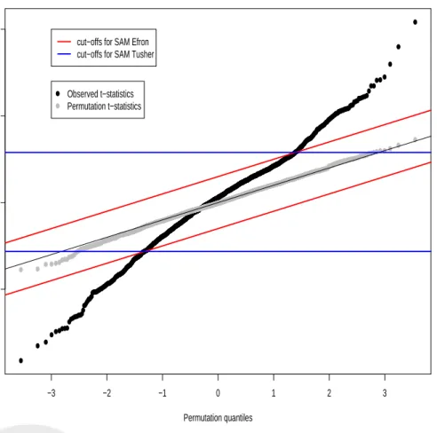
P F ER =E(V|HC0), which leads to the choice of ∆ in each version. In Efron et al., the PFER is estimated by applying exactly the same steps to the original and permuted data,i.e., the PFER is estimated by counting the number of genes with order statistics at least ∆ away from the expected order statistics. In contrast, Tusher et al. compute order statistics only for the original data to obtain global cut–offs for the test statistics. These cut–offs are actually random variables, as they depend on the observed test statistics. In the permutation, the cut–offs are kept fixed and the PFER is estimated by counting the number of genes with test statistics above/below these global cut–offs. Figure 6 gives a graphical representation of the two variants: in the Quantile–Quantile plot of the test statistics, the Efron cut–offs are parallel to the identity line and the Tusher cut–offs are horizontal lines. For a fixed threshold ∆, the two procedures produce different estimates of the PFER. Next, we derive adjusted p–values for the Efron et al. and Tusher et al. procedures. For simplicity, it is assumed that the test statistics are continuous and hence that there are no ties. Also, rather than working with the PFER, we work with the PCER, which is simply the PFER divided by the total number of hypotheses and is a number between 0 and 1.
Adjusted p–values for Efron et al. SAM procedure. For the Efron et al. procedure, let
P CER0ef ron(∆) =E(Vef ron(∆)|HC0)/m=
Pm
j=1pr |T(j)−t¯(j)| ≥∆|HC0
/mdenote the expected proportion of false positives under the complete null for a given threshold ∆. Here, ¯t(j) is taken to be a fixed estimate of E(T(j)|HC0). One may then express the procedure in terms of the following adjustedp–values
˜
p(j)=P CER0ef ron(|t(j)−t¯(j)|), (15) which can be estimated by permutation. Rejection of H(j) for ˜p(j) ≤α controls the PCER at level
α in the weak sense. Since the Efron et al. procedure is based on the distribution of the order statisticsT(j) under the complete null, the subset pivotality condition of Westfall & Young (1993) does not hold. Note that the adjusted p–values ˜p(j) are not necessarily monotone in j, as the differences |t(j)−t¯(j)| are not necessarily monotone. Thus, a test statistic Ti could possibly have a smaller adjusted p–value than a more “extreme” test statistic Tj with |Tj| ≥ |Ti|. A stepwise
version of the Efron et al. procedure could be devised to deal with this feature.
Adjusted p–values for Tusher et al. SAM procedure. Similarly, for the Tusher et al.
procedure, let P CER0tusher(∆) = E(Vtusher(∆) | HC0)/m =
Pm j=1 pr Tj ≥ cutup(∆) | HC0 + pr Tj ≤cutlow(∆)|HC0
/mdenote the expected proportion of false positives under the complete null for a given threshold ∆. One may then express the procedure in terms of the following adjusted
p–values ˜ p(j)=P CER0tusher(∆(j)), (16) where ∆(j)= ( max{t(k)−t¯(k):j ≤k≤j0}, ifj≤j0 max{¯t(k)−t(k):j0 < k≤j}, ifj > j0
for j0 = max{j : ¯t(j) ≥ 0}. Due to the possibility that t(k) −¯t(k) < 0 for some k ≤ j0 or ¯
t(k)−t(k) < 0 for some k > j0, it may happen that ∆(j) < 0 (this problem is not addressed in Tusher et al.). In such cases, the null H(j) is never rejected and we define ˜p(j) = 1. Rejection of H(j) for ˜p(j) ≤α controls the PCER at levelα in the strong sense. Note that the rejection regions
S∆= (−∞, cutlow(∆)]∪[cutup(∆),∞) are nested, that is,S∆0 ⊆S∆for ∆0≥∆. Furthermore, the ∆(j)’s are monotone inj in each of the tails, thus the adjustedp–values are monotone in jfor each tail (unlike thep–values for the Efron et al. procedure). Thep–values are however not symmetric, ast(j) =tand t(j) =−t could correspond to different ∆(j)and cut–offs (cutlow(∆(j)), cutup(∆(j))). Both SAM procedures thus aim to control the PFER (or PCER), but the Efron et al. procedure only controls this error rate in the weak sense. The only difference between the Tusher et al. version of SAM and standard procedures which reject the null Hj for|tj| ≥ c is in the use of asymmetric critical values chosen from the Quantile–Quantile plot (see Braver (1975) for the use of asymmetric critical values). Otherwise, SAM does not provide any new definition of Type I error rate nor any new procedure for controlling this error rate. In summary, the SAM procedure in Efron et al. amounts to rejecting H(j)whenever|t(j)−¯t(j)| ≥∆, where ∆ is chosen to control the PFER weakly at a given level. By contrast, the SAM procedure in Tusher et al. rejects Hj whenevertj ≥cutup(∆) ortj ≤cutlow(∆), wherecutlow(∆) and cutup(∆) are chosen from the Quantile–Quantile plot and such that the PFER is controlled strongly at a given level.
Control of FDR. The term “false discovery rate” is misleading, as the definition in SAM is
dif-ferent than the standard definition of Benjamini & Hochberg (1995): the SAM FDR is estimating
E(V|HC
0)/Rand notE(V /R) as in Benjamini & Hochberg. Furthermore, the FDR in SAM can be
greater than one (cf. Table 3, p. 16 in Chu et al. (2000)). The issue of strong vs. weak control is only mentioned briefly in Tusher et al. and the authors claim that “SAM provides a reasonably accurate estimate for the true FDR”.
Additional comments. The Efron SAM procedure considers the distribution of the order
statis-ticsT(j)under the complete null hypothesis and rejects the null hypothesis H(j)for large deviations of T(j) from its expected value under the complete null. This approach could be refined by ac-counting for the different variances of the order statistics under the complete null,i.e., by declaring genej differentially expressed if|t(j)−t¯(j)| ≥sd(j)∆, where sd(2j)=Pb(t(j),b−¯t(j))2/B. A further