UC Irvine Previously Published Works
Title
Simulating California reservoir operation using the classification and regression-tree algorithm
combined with a shuffled cross-validation scheme
Permalink
https://escholarship.org/uc/item/6vh7s39d
Journal
WATER RESOURCES RESEARCH, 52(3)
ISSN
0043-1397
Authors
Yang, Tiantian
Gao, Xiaogang
Sorooshian, Soroosh
et al.
Publication Date
2016-03-01
DOI
10.1002/2015WR017394
License
https://creativecommons.org/licenses/by/4.0/ 4.0
Peer reviewed
RESEARCH ARTICLE
10.1002/2015WR017394
Simulating California reservoir operation using the
classification and regression-tree algorithm combined
with a shuffled cross-validation scheme
Tiantian Yang1, Xiaogang Gao1, Soroosh Sorooshian1, and Xin Li2
1
Department of Civil and Environmental Engineering, University of California, Irvine, California, USA,2Cold and Arid Regions Environmental and Engineering Research Institute, Chinese Academy of Sciences, Lanzhou, China
Abstract
The controlled outflows from a reservoir or dam are highly dependent on the decisions madeby the reservoir operators, instead of a natural hydrological process. Difference exists between the natural upstream inflows to reservoirs and the controlled outflows from reservoirs that supply the downstream users. With the decision maker’s awareness of changing climate, reservoir management requires adaptable means to incorporate more information into decision making, such as water delivery requirement, environ-mental constraints, dry/wet conditions, etc. In this paper, a robust reservoir outflow simulation model is pre-sented, which incorporates one of the well-developed data-mining models (Classification and Regression Tree) to predict the complicated human-controlled reservoir outflows and extract the reservoir operation patterns. A shuffled cross-validation approach is further implemented to improve CART’s predictive per-formance. An application study of nine major reservoirs in California is carried out. Results produced by the enhanced CART, original CART, and random forest are compared with observation. The statistical measure-ments show that the enhanced CART and random forest overperform the CART control run in general, and the enhanced CART algorithm gives a better predictive performance over random forest in simulating the peak flows. The results also show that the proposed model is able to consistently and reasonably predict the expert release decisions. Experiments indicate that the release operation in the Oroville Lake is signifi-cantly dominated by SWP allocation amount and reservoirs with low elevation are more sensitive to inflow amount than others.
1. Introduction
Reservoirs and dams are the major infrastructures in California for surface water resources management, flood control, and ecosystem protection. Decision makers in California are under increasing pressure because of the emerging unsustainable water-supply problems caused by population growth, environmen-tal degradation, and climate change. California’s severe challenge of meeting rising water demands with limited resources has been widely recognized by decision makers after the state experienced the recent drought [DWR, 2013a, 2013b]. Such a changing situation brought the awareness of policy makers and water management agencies, such as the California Department of Water Resources (CDWR) and the U.S. Bureau of Reclamation (USBR), to timely establish and enforce water regulations and policies to promote water management efficiency in the vast reservoir systems in California. From the downstream water users’ point of view, the amount of upstream inflows to reservoirs might not be sufficient information to establish proper water management plans for agriculture irrigation, ground water pumping, ecosystem protection, etc. To make efficient and prompt water planning, downstream users require a robust estimate on the actual amount water released from an upper-stream reservoir, which are expert release decisions by reser-voir operators.
In order to estimate the controlled releases or storage, which are also termed as reservoir system yields, res-ervoir simulation models are widely used [Louks and Sigvaldason, 1981].Lund and Guzman[1999] concluded that simulation models were more common in practice and, therefore, were more likely to be trusted as a standard compared to optimization models. In early times, Sigvaldson [1976] developed an innovative approach for simulating reservoir responses using a priority ranking concept. Chaturvedi and Srivastava
[1981] developed a screen-simulation model using two types of linear programming methods for a large
Key Points:
AI&DM approaches are useful tools to assist decision making in reservoir management
A newly developed shuffled cross-validation scheme is robust against overfitting
The enhanced CART algorithm is able to reproduce expert reservoir operation decisions Supporting Information: Supporting Information S1 Correspondence to: T. Yang, [email protected] Citation:
Yang, T., X. Gao, S. Sorooshian, and X. Li (2016), Simulating California reservoir operation using the classification and regression-tree algorithm combined with a shuffled cross-validation scheme,Water Resour. Res.,52, 1626–1651, doi:10.1002/ 2015WR017394.
Received 13 APR 2015 Accepted 28 JAN 2016
Accepted article online 2 FEB 2016 Published online 6 MAR 2016
VC2016. American Geophysical Union. All Rights Reserved.
Water Resources Research
complex water resources system. In the recent decades, many advanced reservoir simulation models were developed and became favored by many government agencies and research institutes, such as the HEC-5 simulation model developed by USACE [Bonner, 1989], DWRSIM developed by CDWR [Barnes and Chung, 1986;Chung et al., 1989], the WEAP21 model [Yates et al., 2005], the Calsim model [Draper et al., 2004], etc. As concluded byJohnson et al. [1991], the simulation models were only useful if the operating policies/rules incorporated in the simulation could realistically reflex the actual operation. In practice, reservoirs were always operated by so-called rule curves, which defined an empirically desired reservoir storage-release relationship [Louks and Sigvaldason, 1981]. However, Oliveira and Loucks [1997] pointed out that it was widely acknowledged that system operators often deviated from these rules to adapt to specific condition, objectives, or constraints that may exist at various times, even though the graphic rules provided a guid-ance for reservoir operation.Draper et al. [2004] also criticized that many simulation models were severally restricted by the complex coding of operating rules, which jeopardized the transparency to users. Therefore, in order to enhance the use of reservoir simulation models, it is of great importance of using suitable techni-ques to reproduce the actual release decisions and derive realistic and transparent reservoir operating poli-cies/rules governed by both the traditional hydrological conditions (i.e., inflow, storage volume, precipitation, etc.) and many other nontraditional decision variables (i.e., water delivery and transfer, dry and wet conditions, downstream river stage, etc.).
To reach this goal, the attempts of using artificial intelligence and data-mining (AI&DM) techniques to simu-late reservoir operation have gained much popularity.Kuczera and Diment[1988] developed a WASP (Water Assignment Simulation Package), which employed ‘‘What if’’ logic to explore the operating policy in a water transfer system.Raman and Chandramouli[1996] derived a general reservoir release rules using an artificial neural network algorithm.Shrestha et al. [1996] reconstructed the actual operation rules using a fuzzy-logic approach and compared the generated release with observation.Rieker and Labadie [2012] used a rein-forced learning algorithm to simulate the long-term reservoir operation strategies in the Truckee River of California and Nevada.Hejazi et al. [2008] evaluated the sensitivities of hydrologic information’s time scale and seasonality in reservoir historical releases in California and the Great Plain in U.S.Corani et al. [2009] used a Lazy Learning algorithm to reproduce human decisions in reservoir management in Lake Lugano.
Bessler et al. [2003] extracted the operating rules for a single-reservoir in U.K. using the decision tree rithm, linear regression and evolutionary algorithm, and found out that the results with decision tree algo-rithms were superior over the others. Compared among these three types of approaches,Bessler et al. [2003] also concluded that the decision tree algorithm had an advantage, which allowed the derived rules could be audited and further improved by domain experts. As it is compared to artificial neural network approaches, it is also believed that the simple Boolean logic used in decision tree approaches is more understandable to reservoir operators and easier to practice in real-world application.
Building on these previous works that focus on applying AI&DM techniques to reservoir management, in this study, we attempt to build a simple but efficient decision tree regression model to simulate controlled reservoir releases for nine major reservoirs in California, and investigate the impacts of multiple types of information on reservoir release decision making. In detail, three types of decision tree methods are tested and compared on nine major reservoirs in California, including the Classification and Regression Tree (CART) combined with a newly developed shuffled validation scheme, the original CART algorithm with a standard twofold cross-validation scheme, and a benchmark Random Forest approach [Breiman, 2001].
The objectives of this study are to (1) develop a novel shuffled cross-validation scheme and jointly use with the CART algorithm, (2) apply the enhanced CART algorithm on nine reservoirs in California and compare with the original CART and Random Forest algorithms, and (3) evaluate the influences from multiple deci-sion variables on reconstructing the expert reservoir decideci-sions in California, including the daily releases, storage changes, and trajectories.
Compared to other pioneer studies, we extend the number of decision variables from only hydrological information’s time scale and seasonality [Hejazi et al., 2008] to 15 types of distinct information. Compared to
Corani et al. [2009], in which high accuracy was achieved in reproducing human’s decisions in a single lake in Italy, in this study, we aggressively attempt to reproduce the controlled outflow decisions in nine major reservoirs in California. The technique used in this study belongs to the same algorithm family thatBessler et al. [2003] employed but enhancement is introduced.
This paper is organized into six sections: section 2 provides the information about the nine major reservoirs and the data used. The methodologies, including CART algorithm, Random Forest algorithm, shuffled cross-validation scheme, and Gini diversity index are introduced in section 3. Section 4 presents the simulation results of reservoir controlled outflows, storage daily changes, storage trajecto-ries, and the sensitivity analysis on deci-sion variables. Discusdeci-sion, limitation, and future works are presented in section 5. Section 6 summarizes the conclusions and major findings.
2. Selected Reservoirs and Data
In this study, nine major reservoirs in California are selected, namely, the Trinity Lake, Don Pedro Reservoir, New Excheq-uer Reservoir, Folsom Lake, Friant Reser-voir, New Melones ReserReser-voir, Oroville Lake, Success Lake, and Shasta Lake. Most of the reservoir operation data and hydrological data are collected from the California Data Exchange Center (CDEC), which is an official data-sharing portal used by water agencies, decision makers, and water
Figure 1.Locations of the selected reservoirs with elevations in parentheses (m).
Table 1.Basic Information for Selected Reservoirs, Snow Course Station, and Downstream River Gaugesa
Name River Basin Station Type ID Latitude Longitude Elevation (m) Agency Function Trinity Lake Trinity Res. CLE 40.801 2122.762 722.4 USBR WS, FC, EP Others
S.C. BBS 40.967 2122.867 1981.2 WRD D.G. DGC 40.645 2122.957 487.7 USGS Don Pedro
Reservoirs
Tuolumne Res. DNP 37.702 2120.421 253.0 TID FC, WS, Others S.C. HRS 38.158 2119.662 2560.3 CDWR S/S
D.G. MOD 37.627 2120.988 27.4 USGS New Exchequer
Reservoirs
Merced Res. EXC 37.585 2120.270 267.9 MID WS, FC, Others S.C. STR 37.637 2119.550 2499.4 CDWR S/S
D.G. CRS 37.425 2120.663 50.3 CDWR
Folsom Lake American Res. FOL 38.683 2121.183 142.0 USBR WS, HP, Others S.C. HYS 39.282 2120.527 2011.7 USBR
D.G. AMF 38.683 2121.183 0.0 CDWR S/S
Friant Dam San Quaquin Res. MIL 37.001 2119.705 177.1 USBR FC, WS, Others S.C. NLL 37.257 2119.225 2438.4 SCE
D.G. MEN 36.811 2120.378 51.8 USGS New Melones
Reservoir
Stanislaus Res. NML 37.948 2120.525 346.0 USBR WS, HP, FC, Others S.C. BLD 38.450 2120.033 2194.6 USBR
D.G. OBB 37.783 2120.750 35.7 CDWR
Oroville Dam Feather Res. ORO 39.540 2121.493 274.3 CDWR O/M WS, FC, HP, EP, Others S.C. KTL 40.140 2120.715 2225.0 CDWR O/M
D.G. GRL 39.367 2121.647 28.0 CDWR O/M
Success Dam Tule Res. SCC 36.061 2118.922 210.9 USACE FC, WS, Others S.C. OEM 36.243 2118.678 2011.7 CAL FIRE
D.G. TRL 36.087 2119.430 73.2 USACE
Shasta Dam Sacramento Res. SHA 40.718 2122.420 325.2 USBR WS, HP, EP, Others S.C. SLT 41.045 2122.478 1737.4 USBR
D.G. IGO 40.513 2122.524 205.1 USGS
a
Res.: Reservoir; S.C.: Snow Course; D.G.: Downstream Gauge; WS: Water Supply; FC: Flood Control; HP: Hydropower; EP: Ecosystem Protection; Others: Navigation, Recreation, Groundwater Recharge, etc.; WRD: Weaverville Ranger District; CDWR S/S: CA Dept of Water Resources/Snow Surveys; USBR: U.S. Bureau of Reclamation; USACE: U.S. Army Corps of Engineers; TID: Turlock Irrigation District; MID: Merced Irrigation District; CDWR O/M: CA Department of Water Resources/O & M; SKCNP: Sequoia and Kings Canyon National Parks; SCE: Southern California Edison Company, Big Creek; USGS: US Geological Survey.
users in California. The CDEC installs, maintains, and operates a collection of extensive, centralized hydro-logic operational, and historical data (http://www.water.ca.gov/floodmgmt/hafoo/hb/cdecs/) gathered from various agencies and utilities throughout the United States. Data supporting agencies include the National Weather Service (NWS), the U.S. Army Corps of Engineering (USACE), the U.S. Bureau of Reclamation (USBR), the U.S. Geological Survey (USGS), the California Department of Water Resources (DWR), the Sacramento Municipal Utility District (SMUD), Pacific Gas & Electric (PG&E), the East Bay Municipal Utility District (EBMUD), and multiple local water agencies. In addition, we retrieve the snow depth data and downstream flow information from each reservoir’s nearby snow course station and river gauge station in the down-stream service area, respectively. A summary of selected reservoir, snow course station, and downdown-stream gauge is provided in Table 1. Figure 1 shows the corresponding locations of the selected major reservoirs in California.
The reservoir operation data are categorized into model input (decision variables) and output (target varia-bles). We summarize the types of model inputs and outputs as follows:
1. The first type of model input is the reservoir storage volume, which is widely used by USACE in California as the guidance for reservoir releases. The relationship between releases and storage volumes or water levels is always represented as graphical charts termed as ‘‘rule curves,’’ which represent the empirically desired reservoir operation criteria to meet water supply objective, flood control, and engineering con-straints. It is worth to mention that in model training phase, the storage volume is intentionally lagged for one time step (1 day) for all experiments. It means that current release decisions are based on the ini-tial storage of the day instead of the ending storage of that day, which is similar to the approach employed byRaman and Chandramouli[1996]. In the verification phase, current storage input is calcu-lated by the mass-continuity function using the simucalcu-lated releases on the previous time step (day). 2. The second type of model input primarily includes mostly the traditionally hydrological data for the daily
reservoir operation, such as the reservoir daily inflow, the daily accumulated precipitation (point mea-surement), snow depth in reservoir’s upstream mountain area, and the flow conditions in the down-stream water supplying area.
3. The third type of model input is the wet/dry conditions. CDWR uses the Water Year Index (WYI) for the Sacramento Valley and the San Joaquin Valley to classify the water-supply conditions in a water year. In California, WYI is an important guideline for water planning and management [DWR, 2013b, 2009, 2005]. Officially, the WYIs are determined by the State Water Resources Control Board (SWRCB), which catego-rizes five types of water year: (1) wet, (2) above normal, (3) below normal, (4) dry, and (5) critical year. The calculation and classification examples for WYIs for the Sacramento Valley and the San Joaquin Valley are included in supporting information (SI) for interested readers.
4. Besides the WYIs, there are six different river indices commonly used in California, which are the opera-tional climate predictors forecasted and calculated by CDWR Snow Survey office in the beginning of each water year. According to the communication with CDWR, these indices are also used by other water agencies as indicators for evaluating the climate conditions and operating their facilities for the entire state. More detailed information of these indices can be found in CDWR Snow Survey office. Generally, the calculation of these indices is based on a linear regression method using multiple weather informa-tion, ground-based measurements, and decades of experiences of on-site hydrologists. Namely, the six river indices are the Sacramento Valley’s October–March runoff, April–July runoff, and water year total runoff sum and the San Joaquin Valley’s October–March runoff, April–July runoff, and water year total runoff sum.
5. The fifth type of model input is the State Water Project (SWP) allocation amount. This variable partially represents the influence of policy or law changes related to water transferring and allocation, because the amount of water transferred by SWP must abide with the California Water Codes (laws), agreements, and water rights among multiple stakeholders, and water agencies. In California, the SWP is designated to provide specific amounts of agricultural and municipal water supplies to its 29 agencies over the entire state. However, based on California’s current water-supply condition, the SWP water supply is sub-ject to change over time. Once a change of the prosub-jected water supply is authorized by the governor and the SWRCB, the 29 agencies can only receive and use the officially announced amount of water under jurisdictional rights, unless further announcement is released. For example, on 31 January 2014, the CDWR announced an amendment to the SWP allocation, in which the SWP allocation to farmers and
agricultural water agencies is dropped to 0% due to continuing drought conditions in California. This change of regulation is enforced by California Governor Brown’s drought declaration made on 17 Janu-ary 2014. The infrastructures in California were operating under this action until another announcement was made on 18 April 2014, increasing the SWP allocation back to 5%. These changes in the allocation percentages as a result of the governor’s announcements are retrieved from the California Water Control Board and the SWP official document archive.
6. The last model input concerns the influence of seasonality on reservoir operation, which is the month of a year.
7. The model output (target variable) is the controlled reservoir daily outflow.
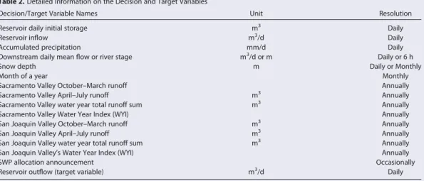
Most of the data for the selected reservoirs cover 16 years from 1 October 1997 to 31 December 2013, except the Trinity Lake (CLE), New Exchequer Reservoirs (EXC), and Shasta Lake (SHA), of which the data start on 24 March 2003, 30 March 1999, and 1 January 2001, respectively. A summary of the decision varia-bles and target variable is provided in Table 2.
3. Methodology
3.1. Classification and Regression-Tree (CART) Algorithm
The method we employ is a white-box and tree-like data-mining technique, termed the Classification and Regression Tree (CART) algorithm, combined with a novel shuffled cross-validation scheme. CART was origi-nally introduced byBreiman et al. [1984], and further developed byBreiman[1996, 2001] into bagging-tree and random forest, respectively. Given a set of decision variables (inputs or predictor) and target variables (outputs), the mechanism in CART is to repeatedly find a classification of the target variable associated with its decision variables based on selected splitting rules so that any new prediction will be the most similar to its observation in terms of the splitting rule defined measurement. The classification tree will eventually divide the whole training data set space into multiple classes (leaves). Each class consists of a set of rules that splits the decision variable spaces. The regression tree takes the average of the target variable values in each class and stores the corresponding splitting rules. Once a new set of decision variable is given to the regression tree, an estimated target value will be returned following the stored splitting rules. In this study, the regression tree is primarily used.
Mathematically, CART is a nonparametric data-mining algorithm capable of predicting continuous depend-ent variable (target variable,~y5Rm) with categorical and continuous predictor variable (decision variables,
~x5Rn). CART uses a binary tree to recursively partition the decision variable space into subsets in which the distribution of target variable is successively more homogenous [Chipman et al., 1998]. Before each split in CART, the prior data set is called ‘‘parent’’ node and the two split sub-data sets are referred to ‘‘children’’ nodes. The partitioning procedure searches through all values of the decision variable~xto find the variable
~xj2nthat provides the best partition of the target variable~yby maximizing the homogeneity of target vari-able~yj~xi~xjand~yj~xi> ~xjin the ‘‘child’’ nodes [Razi and Athappilly, 2005]. The maximum of homogeneity
Table 2.Detailed Information on the Decision and Target Variables
Decision/Target Variable Names Unit Resolution
Reservoir daily initial storage m3
Daily
Reservoir inflow m3
/d Daily
Accumulated precipitation mm/d Daily
Downstream daily mean flow or river stage m3
/d or m Daily or 6 h
Snow depth m Daily or Monthly
Month of a year Monthly
Sacramento Valley October–March runoff Annually
Sacramento Valley April–July runoff m3
Annually Sacramento Valley water year total runoff sum m3
Annually
Sacramento Valley Water Year Index (WYI) Annually
San Joaquin Valley October–March runoff m3
Annually San Joaquin Valley April–July runoff m3
Annually San Joaquin Valley water year total runoff sum m3
Annually
San Joaquin Valley’s Water Year Index (WYI) Annually
SWP allocation announcement Occasionally
Reservoir outflow (target variable) m3
is governed by the selected splitting rule, such as to minimize the summation of relative errors in ‘‘child’’ nodes (equation (1)) [Hancock et al., 2005].
arg minðREðdÞÞ5arg min X L 0 ðyl2yLÞ 2 1X R 0 ðyr2yRÞ 2 ! (1)
whereylandyrare the left and right ‘‘child’’ nodes with L and R numbers of target variables,yLandyRare the mean of resulting target variables in the left and right ‘‘child’’ nodes, anddis the decision or splitting rule governing the partition of the data the decision variable~x. The resulting ‘‘child’’ nodes are recursively partitioned into smaller subnodes until preset stopping criteria are met in the tree-growing procedure. The stopping criteria could be number of iteration, minimum number of samples in final ‘‘child’’ nodes (classes or leaf), or/and maximum of decision tree depth (size). In this study, the minimum number of samples in a leaf is set to 10, the maximum size of decision tree is set to 20, and number of iteration is set to be relaxed. CART has many advantages which could be suitable for reservoir operation and favored by decision makers. The nature of data-driven mechanism of decision tree model provides the transparency in its model frame-work, which allows decision maker to audit and improve the simulation quality [Bessler et al., 2003]. CART is a nonparametric algorithm, in which the simple Boolean logic used in each split is able to provide reasona-ble physical interpretation of historical data. Moreover, the CART algorithm is computationally efficient [Breiman et al., 1984;Lewis, 2000]. The low cost computation characteristic is able to bridge modeling frame-work with the increasing amount of data in the so-called era of ‘‘big data.’’
The applications of CART algorithm, bagging-tree, and random forest are numerous in literature.De’ath and Fabricius[2000] employed CART in analyzing ecological data.Lewis[2000] applied CART in developing clini-cal decision rules.Prasad et al. [2006] used bagging-tree and random forest in ecological prediction. The use of CART algorithm is also very popular in many other fields, such as finance engineering [Fayyad et al., 1996], system-failure detection [Chebrolu et al., 2005], ecosystem modeling [Araujo and New, 2007;Elith and Leathwick, 2009], remote-sensing data analysis [Xu et al., 2005], and reservoir operation [Bessler et al., 2003;
Kumar et al., 2013a, 2013b;Li et al., 2014;Sattari et al., 2012;Wei and Hsu, 2008].Steinberg and Colla[2009] andWu et al. [2008] also summarized that CART is one of the top 10 algorithms in the field of data mining.
3.2. Random Forest
To obtain a good predictive performance, the output classes (tree leaves) have to be high. However, the risk of overfitting the observed data will accordingly increase. One mean to resolve this weakness is to use an ensemble method, such as bagging [Breiman, 1996], boosting [Freund and Schapire, 1996], random forest [Breiman, 2001] etc. Large-scale empirical comparison has been conducted byCaruana and Niculescu-Mizil
[2006], in which the Random Forest algorithm achieved excellent performances compared to numerous supervised learning algorithms. According toLiaw and Wiener[2002], differs from the standard trees, each node is split using the best among a subset of predictors randomly chosen at that node, instead of all deci-sion variables. This counterintuitive strategy turns out to perform very well compared to many other classi-fiers, including discriminant analysis, support vector machines, and neural networks, and is robust against overfitting [Breiman, 2001]. Therefore, in this study, Random Forest algorithm is also employed as a bench-mark algorithm for comparison. Experiments are carried out comparing the observed controlled outflows with the results from random forest, the CART algorithm combined with a shuffled cross-validation scheme, and a standard CART algorithm with twofold cross validation as control run on nine major reservoirs in Cali-fornia. Some settings for the use of random forest are listed as follows: the number of trees in a forest is set to be 200; the number of variables in the random subset at each node is set to be 10; and the minimum of samples in a leave is 1 with the purpose of obtaining a fully developed tree.
3.3. Shuffled Cross-Validation Scheme
A major issue may arise when using the CART model on the data that contain significant random noises. This issue is termed as ‘‘overfitting’’ [Breiman et al., 1984], in which any statistical model, such as the CART algorithm, tends to give a very good or near ‘‘perfect’’ fitting to the training data instead of an accurate estimate of the relationship between the target and decision variables, resulting in a poor predictive capability on a model ‘‘unseen’’ data. To overcome this problem, model ensemble approaches are com-monly used in the decision tree algorithms, such as the strategy adopted in Random Forest [Breiman,
2001]. Using the model ensemble approach, the weak learners associated with poor predictive perform-ances are constantly eliminated in the tree growing process. Different from the model ensemble approach, in this study, we attack the ‘‘overfitting’’ problem of CART by shuffling the training data, and maximizing the posterior performances to select the best model structure, i.e., the decision tree depth. The attempt is to efficiently use limited data to ensure a sufficient number of training samples that con-tain distinct information which are recognizable to the CART algorithm so that accurate predictions on any unseen data can be stabilized.
In order to achieve such a goal, we develop a shuffled cross-validation scheme and jointly use with the CART algorithm. The cross-validation scheme, also called the rotation estimation [Bauer and Kohavi, 1999;
Geisser, 1975, 1993], is a model-validation technique for evaluating predictive performance of a statistical model on an independent or unseen data set [Arlot and Celisse, 2010;Breiman et al., 1984;Burnham and Anderson, 2002;Picard and Cook, 1984]. Several commonly used methods are the hold-out method, the K-fold method [Breiman and Spector, 1992;Kohavi, 1995], and the leave-one/p-out cross-validation method [Allen, 1974;Geisser, 1975;Stone, 1977]. In this section, we introduce the shuffled cross-validation scheme. Generally, the concept is to randomly shuffle the training data and break the training data structure to ensure that the training data set contains even data points that represent all kinds of conditions, such as the operations in dry, wet, and normal years. Different from the random forest concept that the decision variables are randomly selected in developing each individual tree, the proposed scheme first creates many CART models using full decision variables but detects the weak learner (model with poor predictive per-formances) based on the posterior maximum likelihood of model performances on a prepartitioned data sets from the training data sets. In addition, there is no ensemble of multiple trees in the proposed scheme and only one final tree is built using CART algorithm.
Using the proposed scheme, the CART algorithm is iteratively used to develop many decision tree models with different model structures (tree depths). In addition, data are repeatedly shuffled by many times to create many independent training, validating, and testing data sets. The performances of these decision trees on the different shuffled training data sets are evaluated by the Nash-Sutcliffe model-efficiency coefficient [Nash and Sutcliffe, 1970] and stored in an archive. The reasons that we use the Nash-Sutcliffe model-efficiency coefficient are (1) the Nash-Sutcliffe model-efficiency coefficient is a popular measure of the accuracy in evaluating decision tree models [Arlot and Celisse, 2010; Burnham and Anderson, 2002;
Picard and Cook, 1984], and (2) it is a normalized index that addresses the differences between simulation and observation. The commonly used RMSE criterion may not be the appropriate measure given the mag-nitudes of outflows that can vary significantly depending on the size of the reservoirs in the system. Then, a maximum-likelihood method is employed to select the best decision tree model according to model’s predictive performances on a temporary hold-out data set within the whole training data set. The best model is further used to predict the reservoir controlled releases on the test data set, which model never sees during the training and validating period. The purpose of using maximum-likelihood method is to prevent model from giving a nonreproducible good prediction on one single shuffled training data set, especially when the shuffled training data set happens to have similar hydrological conditions with the validating data set.
In order to further illustrate the mentioned shuffled cross-validation scheme, a detailed procedure is listed as: (1) the data are split into a training set and a test set, which is identical to the hold-out method. The training set includes about 80% of the data, and the test set includes the remaining data; (2) the training data set is then shuffled and further split into two subsets, with the first subset containing about another 80% of the training data and the second one containing the remaining data; (3) we iterate one of the struc-tural parameter of CART (decision tree depth) from (2) to user-defined maximum and build a corresponding decision tree model using the first subset; (4) the Nash-Sutcliffe model-efficiency coefficient has been calcu-lated for each model using the second subset; (5) the model with the highest Nash-Sutcliffe model-effi-ciency coefficient is selected, and the corresponding decision tree depth has been stored; (6) the processes of (2)–(5) are repeated for many times (e.g., 50,000 iterations), and the possibility functions of the numbers of candidate models in each tree depth are obtained; (7) the best decision tree depth is chosen based on the highest likelihood of the numbers of candidate models falling into each tree depth; (8) the verification experiment is carried on using the hold-out data set from Step (1). The flowchart of this shuffled cross-validation scheme is shown in Figure 2.
The proposed scheme differs from the cross-validation methodology. The scheme combines the strength of (a) the hold-out methodology, (b) the K-fold method that, in our scheme, K approximately equals to 2, and the data used for training are about 60% of the whole data sets, (c) the leave-p-out method in which the training data set is shuffled and left about 20% of the training data set out, and (d) the maximum-likelihood estimation. The main purpose of combining these techniques is to ensure that the train-ing data contain the proper predict-abilities so that the selected model is able to utilize the historical informa-tion in predicting any model ‘‘unseen’’ (independent) data.
3.4. Gini Diversity Index
In the decision tree growing stage, as the same to all decision tree family, CART relies on the splitting rule that measures how well a split will result in the most homogenous ‘‘child’’ nodes. Two types of splitting rules, namely, the Gini index of diversity criterion and Twoing criterion, are originally intro-duced by Breiman et al. [1984]. The Gini diversity index is a standard and broadly used rule in CART. According toBreiman et al. [1984], the Gini diver-sity index measures the impurity of a node, while the Twoing criterion choo-ses a split that balances the data sets in the ‘‘child’’ nodes, which is not related to a node impurity measure. The use of Gini diversity index in CART is also favored by many researchers in the feature selection problem [Chandra et al., 2010; Guyon and Elisseeff, 2003; Qi et al., 2006; Sandri and Zuccolotto, 2008, 2010] , as well as in the field of reservoir operation [Tsai et al., 2012;Wei, 2012]. Follow-ing these previous works, in this study, we also adopt Gini diversity index as the splittFollow-ing rule in CART and use it as the measure to quantify decision variable’s contribution. According toTimofeev[2004], Gini diver-sity index is calculated by the impurity functioniðtÞshown in the following equation (2):
iðtÞ5X
k6¼l
pðkjtÞpðljtÞ (2)
wherek;l21;2;. . .;Kare the index of the class (leaves);pðkjtÞis the conditional probability of class k pro-vided that is in node t. The maximization of homogeneity of all child nodes will be equivalent to maximiza-tion of change of impurity funcmaximiza-tionDiðtÞ, as shown in equation (3):
arg maxðDiðtÞÞ5arg max 2X K k51 p2ðkjt pÞ1Pl XK k51 p2ðkjt lÞ1Pr XK k51 p2ðkjt rÞ " # (3)
wheretp,tl, andtrare the parent, left ‘‘child,’’ and ‘‘right’’ child nodes, respectively;PlandPrare the probabil-ity of left ‘‘child’’ and right ‘‘child’’ nodes, respectively.
The details of other splitting rules and measurements are available in literatures, such as the Twoing rules [Breiman et al., 1984], the Quinlan’s information gain measure (IM) [Quinlan, 1979, 1986], Marshall Correction [Mingers, 1989], and a random selection of attribute for splitting. The comparisons of different measures are also numerous, such as the works byMingers[1989] andBuntine and Niblett[1992].
4. Results
In this section, experiment settings and simulation results are demonstrated. The simulated reservoir con-trolled outflows are compared with observation under three different scenarios, including CART combined with shuffled cross-validation scheme, original CART with twofold cross validation, and random forest. Using the simulated controlled outflows, reservoir daily storage changes and storage trajectories are further calcu-lated. The contributions of decision variables from different methods are compared using the Gini diversity index.
4.1. Experiment Settings
As introduced in section 2, though the data lengths for the nine major reservoirs in California (Table 2) are not same, most of them are from 1 October 1997 to 31 December 2013. Based on a commonly accepted ‘‘80/20’’ split rule, we hold out the data from 1 January 2010 to 31 December 2013 as test period and the rest are used for training and cross validation. In the shuffled cross-validation scheme, the tree depth for each iteration are set from 2 to 20 and the training data are shuffled 50,000 times, as shown in section 3.3: Steps (2)–(5). This means that there are 700,000 ((152211)3 50,000) candidate decision tree models being constructed and validated using the shuffled training data. The Nash-Sutcliffe model-efficiency coeffi-cient is calculated to evaluate the model performance and compare the candidate models. There are total 19 CART models with tree-depth parameters ranging from 2 to 20 are constructed using 50,000 shuffled training data sets, but not all of the models are qualified to be the candidate model. In each shuffle, one candidate model is obtained by selecting the best one among the 19 CART models. Therefore, after 50,000 shuffles, a total of 50,000 candidate models are created, which fall into 19 types of CART models. Each type of tree contains certain numbers of the candidate model. Figure 3 plots the frequency histograms of candi-date models in the 19 types of CART models applied to California major reservoirs (CLE, DNP, EXC, FOL, MIL, MNL, ORO, SCC, and SHA) using the shuffled cross-validation scheme (red). The best depth for decision tree models applied to the reservoir has the maximum frequency, which indicates that this type of decision tree model is expected to have the most stable and accurate predictive performance on the ‘‘unseen’’ data. The selected depths for reservoirs CLE, DNP, EXC, FOL, MIL, MNL, ORO, SCC, and SHA are 12, 14, 13, 11, 13, 9, 9, 12, and 15, respectively. In Figure 3, the frequency histogram of using CART with a standard twofold cross validation is also shown. The corresponding maximum of the best tree depths for the nine reservoirs are 9, 12, 8, 8, 8, 6, 7, 7, and 9, respectively. A slightly higher tree depth and larger size of tree are chosen when using the shuffled cross-validation scheme. With regard to random forest, the final depths from one random candidate tree are 24, 24, 26, 31, 25, 28, 26, 29, and 29 for the nine reservoirs, respectively.
4.2. Simulation Results for Controlled Outflows, Storage Changes, and Trajectories
Using the selected decision tree depths from the previous section, we test the predictive capability of the decision tree model on the hold-out data set (31 December 2010 to 31 December 2013). The purpose is to examine the actual model’s predictive performance. Because the hold-out data are never used in any train-ing process, here they are considered as an independent future scenario. The closer the predicted outflow to the observation, the better predictive performance the model has. The predicted daily outflows from the nine major reservoirs in California are shown in Figure 4.
To mathematically quantify and compare models’ performance, we chose four statistical measurements suggested byGupta et al. [1998], namely, Root-Mean-Square-Error (RMSE), correlation coefficient (R), Nash-Sutcliffe Model Efficiency (NSE), and Peak Flow Difference (PDIFF). In Table 3, the computed statistics for
nine reservoirs’ controlled outflows simulation are summarized. The formula for calculating the selected sta-tistical measurements are listed as follows:
RMSE5 ffiffiffiffiffiffiffiffiffiffiffiffiffiffiffiffiffiffiffiffiffiffiffiffiffiffiffiffiffiffiffiffiffiffiffiffiffiffi XN i51 ðQobs;i2Qsim;iÞ2 N v u u u u t (4) R5 XN i51
ðQobs;i2Qobs;iÞðQsim;i2Qsim;iÞ
ffiffiffiffiffiffiffiffiffiffiffiffiffiffiffiffiffiffiffiffiffiffiffiffiffiffiffiffiffiffiffiffiffiffiffi XN i51 ðQobs;i2Qobs;iÞ s ffiffiffiffiffiffiffiffiffiffiffiffiffiffiffiffiffiffiffiffiffiffiffiffiffiffiffiffiffiffiffiffiffiffiffi XN i51 ðQsim;i2Qsim;iÞ s (5) NSE512 XN i51 ðQobs;i2Qsim;iÞ2 ffiffiffiffiffiffiffiffiffiffiffiffiffiffiffiffiffiffiffiffiffiffiffiffiffiffiffiffiffiffiffiffiffiffiffi XN i51 ðQobs;i2Qobs;iÞ s (6)
PDIFF5Qobs;m2Qsim;m; m5arg maxðQobs;iÞ;i21;2;. . .;N; (7) where Qsim and Qobs are the simulated and observed outflow, respectively; Qobs and Qsim are the mean of the observed and simulated outflow, respectively; j is the time when maximum peak flow happens during the verification period; and N is the total number of days during the verification period.
In order to further verify the proposed model, despite of the comparison with actual releases, the storage volume changes and storage trajectories are also investigated. Using the simulated outflow and the
Figure 4.Reservoir controlled outflow comparison between observed daily releases (black) with the simulated releases with CART com-bined with shuffled cross-validation scheme (red), CART without shuffling scheme as control run (blue), and random forest (green).
following mass-continuity equation, we calculate the storage volume changes and storage level trajectory for each reservoir during the verification period.
DSt5Inflow2Outflow1Precip:2Evapration1Gain&Loss (8)
St5Sinitial1
Xt i51
DSt (9)
whereDStis the daily storage change at time step t;Stis the storage volume at time step t;Sinitialis the start-ing storage volume.
According to equation (8), the storage daily change equals the total inputs to the reservoir subtracts the total outputs of the system. The precipitation, lake-surface evaporation, and gains and losses data are obtained from the CDEC data sets for each reservoir.
The comparison between the calculated-storage changes and the observed-storage changes is shown in Figure 5 and the corresponding Root-Mean-Square-Error (RMSE), correlation coefficient (R), and Nash-Sutcliffe Model Efficiency (NSE) are presented in Table 4.
According to equation (9), we further calculate the storage trajectories from 31 December 2010 to 31 December 2013, as shown in Figure 6. In Figure 6, the starting storage volume is fixed on 31 December 2010 for reservoirs. The storage trajectories are obtained by accumulating all the simulated daily storage changes throughout the whole verification period. The observations (black line) are the actual daily storage volume archived in CDEC. The corresponding statistics are presented in Table 5.
4.3. Importance of Decision Variables
It is of particular interest to discover which decision variable has the most influence on the reservoir opera-tors’ decisions. As we mentioned above, the Gini diversity index is used to mathematically quantify the con-tribution of decision variables. Generally, according to equations (2) and (3), the smaller the Gini diversity index, the purer a set of ‘‘child’’ node is. The Gini diversity index for a ‘‘parent’’ node is always higher than
Table 3.Root-Mean-Square-Error (RMSE), Correlation Coefficient (R), Nash-Sutcliffe Model Efficiency (NSE), and Peak Flow Difference (PDIFF) Between the Observed Reservoir Controlled Outflow and Simulated Results With Different Methods, Including Combined CART and Shuffled Cross Validation (CART1SCV), CART With Twofold Cross Validation (CART Ctrl), and Random Forest (RF)a
Reservoir Methods RMSE (m3/s) R NSE PDIFF (m3/s)
CLE CART1SCV 16.423 0.919 0.836 5.396 CART Ctrl 27.197 0.745 0.560 2161.452 RF 21.447 0.850 0.720 262.627 DNP CART1SCV 22.688 0.946 0.872 235.762 CART Ctrl 23.695 0.900 0.818 292.142 RF 22.734 0.931 0.861 270.624 EXC CART1SCV 12.034 0.938 0.837 215.118 CART Ctrl 16.142 0.898 0.796 235.426 RF 14.622 0.941 0.833 236.682 FOL CART1SCV 46.937 0.901 0.701 140.299 CART Ctrl 55.217 0.805 0.601 243.043 RF 55.081 0.928 0.726 167.500 MIL CART1SCV 26.452 0.957 0.832 29.226 CART Ctrl 40.659 0.804 0.641 253.703 RF 20.152 0.931 0.848 223.615 NML CART1SCV 13.913 0.913 0.830 22.835 CART Ctrl 16.848 0.906 0.801 258.618 RF 14.707 0.915 0.822 222.901 ORO CART1SCV 34.412 0.960 0.920 85.225 CART Ctrl 65.272 0.852 0.713 2544.229 RF 35.793 0.970 0.959 2120.037 SCC CART1SCV 4.734 0.926 0.811 212.893 CART Ctrl 5.688 0.897 0.735 217.231 RF 4.695 0.900 0.799 216.789 SHA CART1SCV 71.466 0.874 0.742 267.461 CART Ctrl 80.168 0.847 0.701 2964.309 RF 74.627 0.877 0.748 2379.122 a
that of two descendant nodes (‘‘child’’ nodes), which indicates that the employed split using one of the decision variables is able to rationally partition the data and result in a better homogeneity in the ‘‘child.’’ Here we first sum up the Gini diversity index of all resulting ‘‘child’’ nodes for all splits using each decision variable. Then, the summation of the Gini diversity index for each decision variable is normalized to a value between 0 and 1, following the rule that decision variable with smaller Gini index summation has higher normalized value. Such normalization ensures that the decision variable with higher contribution or sensi-tivity in generating the model output has a higher value than others. In other words, the closer the normal-ized Gini diversity to 1, the more efficient and dominating the decision variable is in splitting the target
Figure 5.Reservoir daily storage changes comparison between observed storage changes (black) with the calculated results with CART combined with shuffled cross-validation scheme (red), CART without shuffling scheme as control run (blue), and random forest (green).
variable. Using a pie-graph for each reservoir, we present the normalized decision variable importance from the CART combined with shuffled cross validation, CART control run, and random forests in Figures (7 and 8), and 9, respectively. For better illustration and discussion, the WYIs for Sacramento Valley and San Joaquin Valley in Table 2 are grouped as Dry/Wet conditions, and the six decision variables associated with river indi-ces are categorized as runoff condition. Therefore, there are total nine categories of decision variables, which are compared in Figures 7–9, namely storage, dry/wet condition, runoff condition, SWP allocation, reservoir inflow, seasonality/month, precipitation, snow depth, and downstream river stage.
5. Discussions
5.1. Comparison of Simulated Outflows
As shown in Figure 3, the highest posterior maximum likelihood suggests that the most proper tree size in CART that allows the model has good predictive performances, and more importantly, guaranties model’s stabil-ity on randomly constructed ‘‘unseen’’ data. The distribution shapes of the best tree depth of both CART com-bined with shuffled cross validation and CART control run indicate that either a larger or smaller tree might increase the prediction uncertainty. Similar experiments were presented inBreiman et al. [1984], in which
Breiman et al. [1984] concluded that too small a tree will not use some of the classification information, and therefore result in a large misclassification rate. On the other hand, the misclassification rate originally decreases as tree size grows, and then climbs after it hits a minimum. For our reservoir cases, the proper tree sizes found by the CART combined with shuffled cross-validation scheme are consistently higher than that using CART only (Figure 3), because the shuffling scheme introduces more predictive information which the fixed training data set might not contain. Considering that the number of decision variable is over 10, the levels of tree selected by the posterior histogram are not too high to lose the transparency of the Boolean logic in the decision tree algo-rithm. Comparably, the final tree depths with random forest are significant higher than that with both CART1SCV and CART control run for each reservoir. This indicates that there are more final classes or leaves in random forest than CART algorithms than that with other two methods. In the experiments, all random forests are set to be fully grown and use the best subset of decision variable in each split instead of all variables [Liaw and Wiener, 2002], which is robust against overfitting [Breiman, 2001]. Nevertheless, this strategy in random
Table 4.Root-Mean-Square-Error (RMSE), Correlation Coefficient (R), and Nash-Sutcliffe Model Efficiency (NSE) Between the Observed Reservoir Daily Changes and Calculated Changes Using Simulated Daily Releasesa
Reservoir Methods RMSE (3107m3) R NSE
CLE CART1SCV 0.168 0.959 0.920 CART Ctrl 0.254 0.907 0.817 RF 0.209 0.937 0.877 DNP CART1SCV 0.162 0.944 0.885 CART Ctrl 0.199 0.910 0.827 RF 0.195 0.916 0.835 EXC CART1SCV 5.508 0.069 0.083 CART Ctrl 5.499 0.043 0.067 RF 5.504 0.056 0.055 FOL CART1SCV 0.475 0.800 0.638 CART Ctrl 0.500 0.673 0.447 RF 0.407 0.782 0.652 MIL CART1SCV 0.174 0.879 0.730 CART Ctrl 0.351 0.510 0.092 RF 0.157 0.858 0.727 NML CART1SCV 0.132 0.948 0.876 CART Ctrl 0.156 0.933 0.864 RF 0.146 0.939 0.882 ORO CART1SCV 0.302 0.979 0.958 CART Ctrl 0.568 0.924 0.851 RF 0.398 0.963 0.927 SCC CART1SCV 0.162 0.944 0.885 CART Ctrl 0.199 0.910 0.827 RF 0.195 0.916 0.835 SHA CART1SCV 0.664 0.932 0.854 CART Ctrl 0.703 0.919 0.838 RF 0.624 0.937 0.873 a
forest will consequently produce a final tree with a more complex structure and a higher depth than the stand-ard decision trees. If the tree complexity or the number of final classes is not the primary concern, then the ran-dom forest method is suggested because of its ability to provide diverse predictions. In applying the ranran-dom forest method, it is also important to mention that the higher depths might result in potential loss of logical interpretation for certain splits of decision variables.
According to the comparison of simulated controlled outflows (Figure 4), in terms of the magnitude and variation, the simulated results from all scenarios (CART1SCV, CART control, and Random Forest) are very
Figure 6.Reservoir storage trajectory comparison between the actual storage volume (black) with the calculated results with CART com-bined with shuffled cross-validation scheme (red), CART without shuffling scheme as control run (blue), and random forest (green).
similar to the observation, except the CART control run in MIL, in which numbers of stepwise predictions fail to capture the actual releases. Both of the predicted and observed releases (Figures 4b–4e and 4h) tend to decrease as the drought conditions in California become more severe after 2011. The controlled outflow peaks at the beginning of 2011 (Figures 4a, 4b, 4d, 4e, 4g, and 4i) are well predicted with the proposed method and random forest, while the CART control tends to underestimate (Figures 4d, 4e, and 4i) on almost all the cases. Notably, all methods fail to predict the first high peak in MIL and SCC (Figures 4e and 4h). In the case of SCC (Figure 4h), another following peak (around spring in 2011) is captured by all meth-ods. However, there are some overestimates when using random forest and CART control run. Similar to the case of SCC, all methods fail to predict the first small peak in MIL (Figure 4e). Except CART control run, all other methods are able to successfully capture the second and third peak in 2011. The unsuccessful predic-tion on the first peak in SCC and MIL might be due to some unknown situapredic-tions that current decision varia-bles do not consider, such as an emergent water delivery request from the downstream area, the maintenance of reservoir releasing gates, special reservoir operation during drought condition [Kelly, 1986;
Yang et al., 2015], etc. The model performance could be further improved once historical records about res-ervoir and downstream local information are employed.
It is believed that another important factor that has critical influences on reservoir operation is the water demand. Currently, the water demand is not included in the designed decision variable set due to its avail-ability. We think that even though the water demand from agriculture can partially be represented by stor-age variation and seasonality/month, the actual daily demands from residential, industrial, and agriculture are better predictors. This is because that none of selected reservoirs in the experiment are specifically built only for agriculture water-supply purposes and most of the reservoirs are associated with multiple function-alities. Nevertheless, as mentioned in the previous section, the adding of more influencing and suitable information or predictors is easy and achievable using AI&DM techniques.
The statistical performances of the simulated outflows are satisfactory for all methods. Generally, the NSEs of each reservoir range from 0.560 to 0.959 (Table 3). According toMoriasi et al. [2007], model simulation can be judged as satisfactory if NSE is greater than 0.50 for streamflow. According to Table 3, some reser-voirs are easier to simulated (has higher NSE values) than others. Even though the selected reserreser-voirs have different locations, sizes, and watersheds characteristics, we think that the difficulties in simulating the
Table 5.Root-Mean-Square-Error (RMSE), Correlation Coefficient (R), and Nash-Sutcliffe Model Efficiency (NSE) Between the Observed Reservoir Trajectories and Calculated Trajectories Using Simulated Daily Releasesa
Reservoir Methods RMSE (3107m3) R NSE
CLE CART1SCV 7.092 0.991 0.967 CART Ctrl 21.843 0.941 0.788 RF 13.479 0.979 0.881 DNP CART1SCV 12.404 0.984 0.842 CART Ctrl 13.637 0.938 0.744 RF 14.507 0.977 0.824 EXC CART1SCV 6.434 0.997 0.926 CART Ctrl 12.397 0.973 0.724 RF 22.386 0.945 0.699 FOL CART1SCV 14.480 0.888 0.686 CART Ctrl 25.001 0.844 0.280 RF 11.183 0.903 0.784 MIL CART1SCV 7.471 0.859 0.058 CART Ctrl 28.452 0.438 20.052 RF 13.583 0.630 0.015 NML CART1SCV 21.194 0.976 0.770 CART Ctrl 33.927 0.942 0.411 RF 30.745 0.956 0.516 ORO CART1SCV 17.115 0.991 0.927 CART Ctrl 62.411 0.970 0.300 RF 18.973 0.996 0.935 SCC CART1SCV 12.404 0.978 0.724 CART Ctrl 18.007 0.968 0.642 RF 15.637 0.984 0.714 SHA CART1SCV 26.889 0.969 0.887 CART Ctrl 95.094 0.882 0.103 RF 24.523 0.973 0.933 a
releases are largely due to the reservoir’s functionalities and the predictivity of the decision variables. Most of the selected reservoirs are located along the Sierra Nevada Mountain (Figure 1) and the snowmelt during runoff season is the main supplement for reservoir inflow, the local hydrology’s influences on the operation complexity could be negligible.
As shown in Table 3, CART combined with shuffled cross-validation scheme outperforms the other two methods for four out of nine reservoirs with regard to RMSE and NSE values, while the results for the other five reservoirs are very competitive to the best values generated by either random forest or CART control run. For each reservoir, the RMSE, correlation coefficient, and NSE values with CART with shuffled cross vali-dation and random forest are higher than CART control run, which indicate that these two methods have superior performances over the original CART algorithm in our study cases. Except for FOL, the Peak Flow Difference (PDIFF) calculated with CART combined with shuffled cross-validation scheme is consistently smaller than that with the other two methods. Even though the CART control run can reach smaller Peak Flow Difference value for FOL, the calculated RMSE, R, and NSE are all worse than that with the other two methods. Comparing CART control run with random forest, the latter seems to have better performances on predicting the peak flows, especially for SHA (Shasta Lake) and ORO (Oroville Lake), and random forest has consistent higher correlation coefficient values. In daily reservoir operation, the response to peak flow is always of great importance. When there is a high flow, effective and efficient operation considers the resil-ience of reservoir so that proper amount of water is stored for future sustainable supply. More importantly,
an actual release decision needs to prevent the downstream area from flooding even an increase of release or a deliberate spill is needed. This is also the reason that downstream river stage information from each reservoir’s service area is included as one of the model inputs. With respect to the overall performances on RMSE, R, NSE, and PDIFF, CART combined with shuffled cross-validation scheme will be able to more effec-tively predict the expert reservoir release decisions than the other two methods, especially under peak flow conditions.
5.2. Comparison of Storage Daily Changes and Trajectories
In Figures 5 and 6, the storage daily changes and storage trajectories are presented and the corresponding statistics tables are shown in Tables 4 and 5, respectively. In Figure 5, the calculated storage daily changes from all methods are very close to the observed values, especially for CLE, DNP, EXC, MNL, ORO, and SHA (Figures 5–5c, 5f, 5g, and 5i). The major discrepancies between the simulated values and observation hap-pen in predicting three positive peak changes in FOL, two negative changes in SCC (Figures 5d and 5h), and some midlevel changes in MIL (Figure 5e). The differences are mainly due to the discrepancies between observed and simulated releases (Figure 4), as well as the errors in quantifying the losses and gains in each reservoir, such as the overestimates on reservoir evaporation, and unmeasured tributary inflows to reser-voirs, which tend to cause positive changes in daily storage. Comparing the RMSE, R, and NSE values in Table 4, CART with shuffled cross-validation scheme overperforms other two methods in CLE, DNP, ORO,
and SCC, while random forest is superior over other two in SHA. With regard to other reservoirs, the statistic values with CART with shuffled cross-validation scheme and random forest are competitive and slightly bet-ter than the CART control run.
Using the storage daily changes, the storage trajectories are further calculated with a forced starting value (on 31 December 2010) for reservoirs. Figure 6 shows the comparison between the calculated storage tra-jectories and observed storage volume. The corresponding RMSE, R, and NSE values are shown in Table 5. As shown in Figure 6 and Table 5, CART control run seems to give the worst simulation results of storage trajectory, and the differences to observation are relatively larger than the other two methods, especially for FOL, MIL, ORO, SCC, and SHA (Figures 6d, 6e, and 6g–6i). Random forest is able to give better results than the CART control run and the simulation results are similar to that with CART combined with cross-validation scheme in CLE, DNP, FOL, ORO, and SHA (Figures 6a, 6b, 6d, 6g, and 6i). In some cases, such as EXC, MIL, NML, and SCC (Figures 6c, 6e, 6f, and 6h), the simulation results with CART combined with shuffled cross validation are slightly better than that with random forest. According to the statistics presented in Table 5, CART with shuffled cross-validation scheme is able to produce better RMSE, R, and NSE in five out of nine reservoirs, including CLE, DNP, EXC, MIL, NML, and SCC. Random forest overperforms the other two methods in FOL and SHA. For CART control run, a dramatic discrepancy in matching actual storage trajecto-ries is observed in MIL. The primary reason is the failure of predicting the magnitude and variations of
discharges during 2011. The differences between simulated and observed daily releases accumulate over time and result relatively large discrepancy in storage trajectories. Generally, the results produced by CART with shuffled cross-validation scheme can reach the best statistics for most of the study cases as compared to other methods, and the calculated storage trajectories using the proposed method are significantly closer to observation than the CART control run.
Due to the fact that the storage trajectory is calculated by accumulating the daily storage changes to the starting storage volume, errors in certain days might be cancelled with each other. For example, an overesti-mate on the first day and an underestioveresti-mate on the second day might induce a near-perfect storage volume on the third day. Another potential uncertainty source is the autoregulation characteristics of the model. A fully regulated or perfectly trained model would produce a storage trajectory that repeatedly crosses the actual storage trajectory, such as only limited periods shown in the CLE, FOL, SCC, and SHA cases (Figures 6a, 6d, 6h, and 6i). In an ideal case, a given model may predict a low release once the storage volume is low and a high release when the storage volume is high. Such a model could regulate the simulated storage volume to remain within an acceptable uncertainty range. However, the autoregulation effect could be weakened by different model settings. In our designed experiment, the temporal resolution is daily and storage volume is only 1 of the 15 variables. Therefore, the model’s autoregulation capacity is limited. For example, model might find out daily inflow to be more strongly correlated with daily release decisions than the storage volume. This is because the actual release contains relatively high noise while storage variations are always slower and smoother.
Even though the two facts mentioned above might result in errors and uncertainties in storage trajectories, a robust storage trajectory calculation employed in this study is still able to give decision makers certain confidence in evaluating the model performances, especially for seasonal time scale or shorter prediction lead time. As the confidence in the quality of input data deteriorates, shorter prediction or simulation time scales will become more realistic and operational, such as seasonal scale or weekly scale. Shorter time scale simulation will allow users to recursively test model performances and gradually adjust model settings and forcing data. Longer period of simulation will inevitably bring more uncertainty in the results and cause hes-itations from decision makers to practically use the AI&DM techniques. Nevertheless, the validation and test should be conducted in relatively long time scale, such as years, to expose both pros and cons of any pro-posed simulation model.
5.3. Reservoir Operation Patterns
As mentioned in section 3.4, the decision variables contributions are measured by the normalized Gini diversity index, which allows a sensitivity analysis of the decision variables and discoveries of certain reser-voir release patterns. According to Figures 7–9, one interesting finding is that without any prior information, all methods consistently detect that the historical release decisions in the Oroville Lake are very sensitive to the changes of SWP allocation. On average, the SWP allocation explains over 24% of the total variations of ORO’s releases decisions according to Figures 7–9. As the most vital fresh headwater supply source for the SWP delivery, the Oroville Lake provides about 4.3173109m3of water every year to 29 state water agen-cies in the central and southern parts of California. The SWP water delivery obligation makes the Oroville Lake very unique among all the nine reservoirs. The contribution percentage of SWP allocation amount ranks as the second largest one among all decision variables and the decision variable with the largest con-tribution is the downstream river stage.
Different from the consistent model results in ORO, both CART combined with shuffled cross validation and random forests find out that the contributions of SWP allocation are about 10% and 15% in explaining the historical release patterns in the Shasta Lake (Figures 7i and 9i) and Trinity Lake (Figures 7a and 9a), respec-tively. Comparably, CART control run shows there is nearly 0% contribution from SWP allocation (Figures 8a and 8i). The Shasta Lake and the Trinity Lake (CLE) are the largest and second largest reservoirs, respectively, in the California’s Central Valley Project (CVP). Part of the SHA and CLE releases will flow to the Sacramento River and merge with the water from the Feather River. Eventually, the merged streamflow is jointly used and delivered to the Central and Southern California for agriculture, residential, and ecological uses, accord-ing to the multiagencies water sharaccord-ing agreements between SWP and CVP [DWR, 2005, 2009, 2013b;USBR, 2004]. Therefore, it is reasonable to infer that the SWP allocation can also impact the reservoir operation decisions in both Shasta Lake and Trinity Lake. The contributions of SWP allocation could be limited in these
two reservoirs as compared to the main headwater source of SWP, which is Oroville Lake. According to Fig-ures 7 and 9, the contributions of SWP allocation on the release decisions in SHA and CLE are estimated to be 10–15% lower than that in the Oroville Lake. The fact that CART control run fails to detect the influence from this variable in SHA and CLE is mainly due to that the best tree depth of CART control run reaches maximum values around 9 and 7 for CLE and SHA, respectively. The final tree depth with CART control run is consistently smaller than that with other two methods (Figure 3). The trees developed by CART control run might not be fully grown or even not using the SWP allocation variable in splitting the training data. Another interesting finding is that the reservoir inflows play a more important role in the reservoirs with lower elevations. According to Figures 7–9, the contributions of inflows account for over 50% of the total variation of the release decisions in FOL and MIL, which is in agreement among all methods. Surprisingly, FOL and MIL are the two reservoirs with the lowest elevations as compared to others. The elevations of FOL and MIL are 142 and 177 m, respectively (Table 1). It is believed that for the low-elevation reservoirs, the operation rules turn to be more simplistic when it is compared to those in high/medium elevation reser-voirs. With less risk of being suffering from flooding, the priority of water supply for low reservoirs becomes higher. Moreover, low-elevation reservoirs have fewer obligations to transfer water to other areas, because they are already closer to water demand areas, such as farmland, residents, and industry, as compared with high/medium elevation reservoirs. The operation rules for these reservoirs are mostly to mitigate the defi-ciency between the available water and demands. In other words, the management of the outflows depends mostly on the available water that these reservoirs receive from upper-stream area, which is the inflow amount. Despite of the agreement that all methods detect inflow is the most important variable in explaining releases in FOL and MIL, the inflow contribution estimations with CART control run are relatively higher than that with the other two methods. In the case of MIL (Figure 8e), the CART control run quantifies that the influence from seasonality on release decisions is about 3.75%, which is significantly smaller than the estimates from CART with shuffled cross validation (Figure 7e) and random forests (Figure 9e). Because the Firant Dam (MIL) is located in the central valley area of California (Figure 1), where agriculture activities and farm lands are intensive, the seasonal demands for irrigating crops can significantly impact MIL’s release decisions. Even though the CART control run underestimates the influences from seasonality, the contribution from downstream river stage is found to be significantly larger than that with other two meth-ods. It is possible that the seasonality changes are also embedded in the variation of downstream river stage. The dependence among decision variables will be further discussed in the next section.
With regard to the low-elevation reservoirs, we further investigate the extreme case of the Folsom Lake, in which models show that the inflow is largely dominating over 80% of the reservoir release decisions. We find out that the spill events in Folsom Lake are more frequent and intensive than other reservoirs. During the spill events, most of the rule curves designed for flood control, water supply, or hydropower generation will be no longer applicable, and the inflow and outflow are almost equivalent to each other, which results in a high correlation between inflow and outflow. However, the high dependence between these two varia-bles does not undermine the argument that sometimes the storage-release rule curve has its limitation and might not sufficiently represent the actual release decisions. We think that the use of AI&DM techniques, which directly fits the actual releases with multiple decision variables, is able to rationally mimic the histori-cal expert reservoir operation and provide transparent and logihistori-cal representation of daily decision making process.
According to the Figures 7–9, it is also noticed that the operation of many reservoirs rely on the down-stream river stage. We infer that it is because the downdown-stream status is very crucial to release operation dur-ing high flow periods. Traditional flood control rules are highly dependent on seasonality and may have different rule curves for various months. However, if the downstream river status already exceeds a certain level and the reservoir storage-based rule curves still allow extra releases, the reservoir operator has to intentionally reduce the releases, therefore, deviate from the predefined graphical operating policies/rules. We also expect that there are other similar situations that the actual releases are different from a predefined rule curve, such as when an urgent water delivery requests are made by downstream users, or a change of SWP allocation, or a facility suddenly temporarily becomes off-line.
Also, we carried out a sensitivity test of removing downstream gauge information from the experiments. We found out that the contribution of seasonality/month dramatically increased for the Oroville Lake (ORO), New Melones Reservoir (NML), and Trinity Lake (CLE), which indicated that the downstream river stage