UC Merced
UC Merced Electronic Theses and Dissertations
Title
Optimization Framework For Improved Comfort & Efficiency
Permalink https://escholarship.org/uc/item/3p37v8xh Author Yadav, Ashish Publication Date 2019 Peer reviewed|Thesis/dissertation
University of California
Merced
Optimization Framework For Improved Comfort &
Efficiency
A thesis submitted in partial satisfaction of the requirements for the degree
Master of Science in Electrical Engineering and Computer Science
by
Ashish Yadav
c
Copyright by Ashish Yadav
The thesis of Ashish Yadav is approved.
Stefano Carpin
Wan DU
Alberto E. Cerpa, Committee Chair
University of California, Merced 2019
Table of Contents
1 Introduction . . . 1
2 Related Work . . . 7
2.1 Occupancy Detection & Prediction . . . 8
2.2 Occupant Comfort . . . 10
3 System Requirements . . . 13
3.1 Human Thermal Comfort . . . 15
3.1.1 Conditions of the occupant study . . . 15
3.1.2 Comfort App Design . . . 16
3.2 Occupancy Detection & Prediction . . . 18
3.3 System Identification . . . 22
4 Model Predictive Control . . . 26
4.1 Optimization Constraints . . . 26 4.2 Objective function . . . 27 5 System Implementation . . . 30 6 Case Study . . . 35 6.1 Environmental Conditions . . . 35 6.2 Performance Metrics . . . 36 6.3 Model Accuracy . . . 38 7 Results . . . 41
7.1 Thermal Comfort Analysis . . . 41
7.2 Cost and Energy Analysis . . . 45
7.2.1 Cost Analysis —& Energy Analysis . . . 47
8 Discussion . . . 49
9 Conclusion . . . 51
List of Figures
1.1 Energy consumption in a building: 2017 (US) . . . 2
1.2 HVAC System Architecture . . . 3
2.1 OFFICE System Overview . . . 8
3.1 Comfort voting page (left) and feedback (right) . . . 14
3.2 Comfort Voting page in web format . . . 16
3.3 Drift strategy setpoints to save energy . . . 17
3.4 Actuated flow (CFM) as occupancy changes . . . 18
3.5 GridEye Sensor before deployment . . . 19
3.6 8x8 thermal array sensing an occupant . . . 20
3.7 Occupancy sensors before deployment . . . 22
5.1 OFFICE System Architecture . . . 31
5.2 OFFICE Grafana Node Map . . . 33
5.3 OFFICE Zone Temperature Plots . . . 34
6.1 3-D Model of building . . . 36
6.2 Temperature prediction versus ground truth . . . 37
6.3 Model error characteristics for each zone . . . 38
6.4 Zone 1: Temperature prediction versus ground truth . . . 39
7.1 Example of thermal comfort for all zones in WebCTRL . . . 42
7.2 Thermal preferences vote distribution for the users in our building. Val-ues [-3,-2,-1,0,1,2,3] corresponds to [Cold, Cool, Slightly Cool, Neutral, Slightly Warm, Warm, Hot] in our comfort app. . . 44
7.3 Zone temperature variation across the day for all zones for a selected day 44 7.4 Votes distribution in our comfort app as a function of the time of the
day. . . 46 7.5 Operation cost of OFFICE vs WebCTRL . . . 47 7.6 Energy consumption of OFFICE vs WebCTRL . . . 48
List of Tables
3.1 MPC variables and descriptions . . . 24
7.1 Room thermal satisfaction survey report . . . 41
7.2 Quality of Thermal Comfort . . . 42
Acknowledgments
First, I would like to thank my advisor Alberto Cerpa for his support and guidance throughout my graduate study. I am also thankful for the delightful company and help of my colleagues, Alex Beltran, Daniel Winkler and Claudia Chitu who demonstrated to me what an excellent graduate student is supposed to be. I would also like to express my gratitude to my parents, Shiv Ram Yadav and Neelam Yadav, and my brother, Manish Yadav for their loving support and I am thankful to my wife, Suhani Nagpal for her trust and believing in me and making this work possible and my time at UC Merced all the more enjoyable.
Specifically, I would like to acknowledge the work included in this thesis which were co-authored by myself, my peers, and my Advisor. All chapters are based on our recent submission to Sensys ’19. Section 3.2 of Chapter 3 is based on the publication, OBSERVER [ECC14], with primary author Varik L Erickson who used to work in the same lab. Section 3.1 is based on the publication Thermovote [EC12]. And once again, Professor Cerpa and Daniel Winkler who helped make all the above possible with guidance and editing.
I would like to thank and show my appreciation to all people involved in this project, for their volunteer time and valuable participation: from the personnel work-ing in the buildwork-ing where this project took place to the assistant director from Facili-ties Management Team, James Brugger for his unconditioned support and expertise. Special thanks to Alex Beltran for his very important contributions and collaboration.
Vita
1989 Born, Himachal Pradesh, India 2007-2011 Bachelor of Technology, Computer Science, Jaypee University of Information Technolog. Himachal,India
2012-2017 Technical Associate, SpurTree Technologies–Bangalore,India. 2017-2019 Master of Science, Electrical Engineering and Computer Sci-ence, University of California–Merced.
Publications
Ashish Yadav, Ahmed Sabbir Arif, Effects of Keyboard Background on Mobile Text Entry, In Proceedings of the Effects of Keyboard Background on Mobile Text Entry(MUM 2018) Nov 2018.
Abstract of the Thesis
Optimization Framework For Improved Comfort &
Efficiency
by
Ashish Yadav
Master of Science in Electrical Engineering and Computer Science University of California, Merced, 2019
Professor Alberto E. Cerpa, Chair
The Internet of things (IoT) is the extension of Internet connectivity into physical devices and everyday objects. Embedded with electronics, Internet connectivity, and other forms of hardware (such as sensors), these devices can communicate and interact with others over the Internet, and they can be remotely monitored and controlled [Wik19].
The term internet of things has evolved by many fold due to convergence of multi-ple technologies like machine learning, embedded systems, wireless-sensors, real-time analytics, etc. A growing number of IoT devices are being developed for consumer use, including connected vehicles, home automation, wearable technology, connected health, and remote monitoring devices. We want to apply some of these technologies and techniques to make commercial spaces smarter.
Buildings are responsible for a significant portion of energy consumption in the US, accounting for more than 40% of US primary energy consumption. Heating, ventilation and air-conditioning (HVAC) accounts for nearly 50% of that use. Con-ditioning buildings is important since people spend 87% of their time in the place they live (residential) and the place they work (commercial). Despite this massive expense, many users are dissatisfied with the thermal conditions in buildings. Savings
made in HVAC systems therefore have a major impact in energy consumption and cost, together with reduction of greenhouse emissions for the nation. Equally critical is to provide thermal quality of service to their users, so people are comfortable in the place they reside and work.
In this thesis, we explore the trade off between commercial building HVAC energy consumption and the quality of thermal conditioning provided to users. We argue that optimal HVAC control cannot be achieved due to lack of critical information, namely where the users are inside the building,what do they want with respect to thermal comfort and how each zone responds to thermal changes. In this work we present OFFICE,a model predictive control (MPC) framework for smart building HVAC control. The framework has several components that help addressing the current HVAC control systems shortcomings, including
1. occupancy sensing in real-time
2. occupancy prediction models based on historical occupancy data 3. human-in-the-loop comfort feedback
4. data-driven thermodynamic building models, and 5. weather forecasting data
All these components provide the necessary input to our model predictive control optimization framework that minimizes monetary costs in energy use while maintain-ing quality comfort bounds for the buildmaintain-ing’s users based on real-time user’s feedback. We developed a large system that involves all the above components, replacing the Building Management System control algorithms, taking over full control of the HVAC system. We tested our framework OFFICE in a real LEED Gold certified university building with over 20 workers performing their daily tasks for 4 weeks, and we showed that we could obtained monetary costs savings of more than 10% while at the same
time reducing the users’ dissatisfaction levels with thermal comfort from 25% to 0% dissatisfaction, significantly improving the quality of thermal service provided to the building’s users.
CHAPTER 1
Introduction
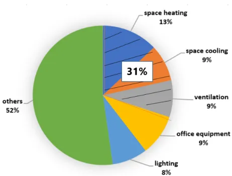
Buildings are an essential piece of our daily lives and individuals invest 87% of their energy inside buildings [KNO01]. To keep up the thermal comfort in buildings, a lot of vitality is utilized to condition these spaces. In the US buildings represent 40% of energy utilization [Adm] and of that half of energy goes to heating, ventilation, and cooling (HVAC) [D12] Figure 1.1.
The goal of conditioning office spaces is largely missed since 75% of occupants report that they are dissatisfied with their thermal comfort [EC12]. In addition to uncomfortable occupants, a common issue is that spaces are conditioned whilst they may be unoccupied, or not ventilated appropriately based on the real quantity of occupants inside the room, losing enormous energy.
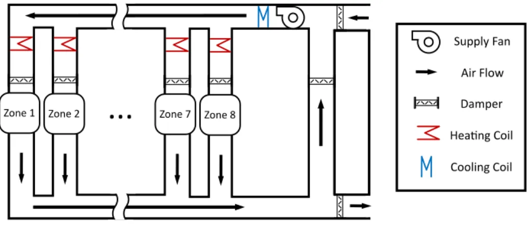
In the US, 88% of the large commercial building stock has centralized HVAC systems [D12]. The most prevalent HVAC system is the single duct terminal reheat, which is composed by an Air Handler Unit (AHU) that is a big fan (usually located on the building’s roof) and heating and cooling coils that can modify the air’s tem-perature, and Variable Air Volume (VAV) boxes that take this pre-conditioned air from the main duct, heat it if necessary (thus the terminal reheat), and control the air flow provided to its controlled zone. The air is mixed in each zone and excess air is returned by the return duct (which may have an additional fan). In many instal-lations, the returned air goes to an economizer, which decides to recirculate a certain percentage of the air in order to save energy. Figure 1.2 shows the basic HVAC system architecture.
Figure 1.1: Energy consumption in a building: 2017 (US)
It is vital to point out that the principal intention of HVAC systems is to provide thermal comfort to its occupants, and doing it in an energy efficient way that min-imizes power cost. So there is a clear trade-off in this situation, where in order to satisfy user thermal comfort requirements, the system must spend energy, which we ultimately want to minimize. If the only goal is to reduce energy consumption, the solution to this problem is simple, since we would simply turn off the HVAC system completely. We would also like to point out that by controlling both air flow and air temperature, the VAV achieves thermal comfort in each zone. Given the initial condi-tions (zone temperature) and the zone’s thermodynamic model, the VAV´s objective is to achieve a potentially new zone temperature in a finite amount of time. This goal can be achieved in many ways, and the set of possible solutions can be depicted by a line in the air flow and temperature two-dimensional space, where any point in the line provides a viable solution to the problem. For example, if a zone is too cold for user comfort and we need to increase the zone temperature, a possible solution could be providing a small value of air flow, but with an air temperature much hotter
...
Zone 1 Zone 2 Zone 7 Zone 8
Supply Fan Air Flow Damper Heang Coil
Cooling Coil
Figure 1.2: HVAC System Architecture
than the zone goal temperature, such that after the hot supply air provided and the zone’s air is mixed, the zone’s temperature will increase and reach our goal temper-ature. Another solution could be to supply air that is only slightly hotter than our goal temperature, but increase the air flow significantly, achieving the same result. To make matters a little more complicated, zones are also controlled for ventilation requirements, which means that the variable air flow is also restricted by minimum flow requirements to remove the buildup of CO2 in the zone.
In this thesis, we argue that we need three pieces of information currently missing
in all HVAC systems to design a system that minimizes energy costs subject to comfort constraints:
(a) the distribution of occupants in all the zones/rooms (both real-time and fu-ture),
(b) the thermal preferences of the occupants, and (c) the thermodynamic model of each zone.
In other words, we need to know where users are (and will be), what users want, andhow each zone responds to changes. Currently, this information does not exist or is not available to HVAC engineers defining the operational control rules of the HVAC
systems. The state-of-the-art in building control is to make certain assumptions to fill this gap. First, occupancy is assumed to be homogeneous in all zones to maximum occupancy, so adequate ventilation levels can be set during the building “occupied hours”. Second, what constitutes a comfortable temperature range is defined by the facility manager in an arbitrary way during “occupied hours”, and those bounds are relaxed during the rest of the time (“unoccupied hours”). Finally, the HVAC control rules do not take advantage of any knowledge of the zone dynamics (e.g. loads, external walls insulation, solar gain, etc.), and they assume that the VAV boxes have been properly sized and configured at commissioning time when the building was constructed, and no changes to walls or internal space configuration have happened. Clearly, many of these assumptions are violated in practice, which leads to users being uncomfortable and building energy bills being higher than they should be.
It is not enough to know whether a room is occupied or not as previously explained in [ECC11], but rather it is critical to also know the actual number of occupants. This is because we can control the ventilation rate if we know the actual occupancy count based on ASHRAE 62.1 standard [ASH07b] and we can provide better thermal conditioning strategies with this information. In addition, since the time it takes to condition a room may be orders of magnitude larger that the time it take users to move from one zone to another one, we need to predict the movement of building’s users in order to do pre-conditioning ahead of time. In our work, we leverage previous work in occupancy sensing [BEC13] and occupancy prediction [ECC14] to solve the answer to the question where users are (and will be).
In addition, we also leverage previous work related to human-in-the-loop feed-back [EC12,WBE16] in order to get real-time estimation of users comfort requirements to address the question what users want. Note that by catering to any comfort needs of any user, we expect our solution to satisfy their quality of service requirements at the expense of potentially increasing energy use and cost.
constantly collects data from building to find the optimum parameters of a gray-box model approach based on physical thermodynamic principles and model parameters from the data to answer the question of how each zone responds to changes.
OFFICE integrates all the above data together with weather prediction data into a MPC framework. Our system minimizes the cost of HVAC energy subject to the physical limitations of the HVAC system, the thermodynamic model learned from the system identification procedure, the user’s real-time and predictive occupancy, the user’s real-time comfort feedback and the current and predictive weather to achieve the best energy efficiency cost subject to the thermal comfort constraints of the user.
We would like to highlight the main contributions of our work as follows:
1. We develop a novel model predictive control (MPC) framework that optimally manages the trade off between energy cost and quality of comfort to the building users, by including input data from where users are (and will be), what users want, how zones react to changes, and current and forecast weather data. 2. We develop a novel data-driven system identification process together with a
gray-box thermodynamic model, that it is simple enough to run in a control loop, yet powerful enough to permit sensible control decisions of the thermal zone.
3. We evaluate the system under realistic conditions in a LEED Gold certified building1 [Cou17], which is being used by 20+ users in their daily tasks. We compare our results with the best control strategies designed by experienced building HVAC engineers, showing a significant improvement in both quality of thermal comfort to the users and overall energy cost.
To our knowledge, this is the first work that combines occupancy sensing and
1LEED: an acronym for Leadership in Energy and Environmental Design. The U.S. Green
Build-ing Council’s LEED green buildBuild-ing program is the preeminent program for the design, construction, maintenance and operations of high-performance green buildings in the U.S.
prediction, human comfort feedback, data-driven thermodynamic models and weather forecasting into a holistic framework for HVAC building control.
The rest of my thesis is organized as follows: Chapter 2 shows the related work, Chapter 3 explains the main components that feed into our framework. Chapter 4 explains in detail the model predictive control framework, and Chapter 5 discusses system implementation details including the building communication interface for sensing and actuation. Then, Chapter 6 explains the conditions of the experiments, and Chapter 7 presents the results of the performance evaluation. Chapter 8 discusses the results and limitations of the system, and finally Chapter 9 concludes.
CHAPTER 2
Related Work
The use of MPC for HVAC control has been explored in the literature before [KMB13a, MKD12, KB11, MMB15, SGM16, CAN14, SFC18]. MPC is a very popular model be-cause it provides opportunities for optimal energy management in HVAC control, being suitable in situations of conflicting constraints and objectives, such as physical constrains of the building, and indoor comfort ranges. However, most of this work has been done from a theoretical control theory point of view, with the experimentation mostly done in simulation.
In addition to traditional MPC models, work has been done in [MB12, PVR13, PMV13] to build a stochastic model predictive control. These efforts focus on un-certainty of occupancy and thermal load predictions and minimization the time the system falls outside the comfort ranges while optimizing the energy use. None of these systems do occupancy detection but consider occupancy as part of the load of the system, even though greater savings can be achieved with demand-response ven-tilation when occupancy is taken in consideration. In our work, we use deterministic MPC, i.e., whenever we have probability distribution functions to model our system inputs and constraints, we take the most likely value instead of using the full distribu-tion of values. However, as we mendistribu-tioned above, we consider a wider range of inputs into our MPC framework than this related work, including real-time and predictive occupancy, real-time user comfort feedback, data-drive thermodynamic zone models and weather forecasting to solve the optimization problem. While we could have used the more powerful stochastic MPC framework in our formulation, we decided to leave
Figure 2.1: OFFICE System Overview
this for future work.
2.1
Occupancy Detection & Prediction
Due to its importance for the MPC, suitable approaches for occupancy estimation and forecast were studied extensively [ECC11, MCM12, EAC13, BEC13, ECC14, SAS17]. In [KJD09], the authors explore the use of cameras to estimate occupancy. They do not, however, address how cumulative error can affect estimates of occupancy. Even a single error will cause error to propagate forward, as mentioned above. The total ground truth for different times of the day was also limited to a total of 4 hours.
Cameras are also used as optical turnstiles by the authors of [EAC]. In order to measure occupancy for several areas, they mount multiple strategically placed cam-eras in hallways. Unlike [KJD09], however, they discuss cumulative error reduction strategies. To estimate the error, they impose maximum occupancy limits and use a
particle filter with a live data occupancy model. However, since their approach uses a model, their approach also requires a non-trivial amount of ground truth occupancy data (2 weeks), collected using webcams. The occupancy RMSE achieved was 1.83 persons, more than 5 times the ThermoSense’s [BEC13] error.
In [BLT10], occupant counts are achieved by counting peaks within the his-tograms, as well as PIR sensors in order to detect occupancy for certain areas and elderly people are tracked using Imote2 motes with Enalab cameras and utilizing a motion histogram for a period of 1 week. Since the camera has to continually poll the room to generate the histograms of motion, the power consumption will be high during occupancy periods. This system also has the privacy issue ; cameras need to be placed directly in the room.
The authors of [SBK11] use active radio frequency identification (RFID) tags to determine occupancy instead of relying on PIR sensors alone. The limitation of this strategy is that each occupant must have an RFID tag and that tag must be co-located with the occupant at all times.
The papers [LSS10, ABD11] describe methods that uses door sensors with PIR sensors to obtain a binary measurement of occupancy. They minimize instances in which overly still occupants become invisible to the PIR sensor by adding door sensors. Although this technique improves binary occupancy measurement, these systems do not provide an accurate estimate of occupancy.
The papers [LHD09, MMC11] estimates occupancy by measuring a variety of pa-rameters.For 5 and 1 week deployments, they collected ground-truth data using video camera and a voluntary electronic tally counter for the user to measure room occu-pancy. In these deployments, they utilize multiple sensors to estimate occupancy; CO2, CO, lighting, temperature, humidity, motion, and acoustics. They define mul-tiple feature vectors for each parameter, which are then used to estimate occupancy with multiple models. While this multi-sensor approach works well for occupancy es-timates alone, when combined with a ventilation strategy, this approach will not work
well. They assume that room occupancy estimates will not be affected by ventilation. However, as ventilation will affect CO2 and humidity levels and therefore occupancy estimates, ventilation rates based on occupancy estimates from this system are likely to result in wild fluctuations in ventilation actuation and underventilation periods. In this case, even with the known calibration and response time problems [FFS06], ven-tilation is better controlled directly by CO2 sensors. Essentially, if CO2 or humidity is used as a sensory input, either you can control ventilation or estimate occupancy, not both at once.
The work in [GIB12] was the first attempt to quantify the inclusion of occupancy data with an MPC control strategy, showing its great potential via simulations. This was followed by [BC14], which used a very specific occupancy sensor infrastructure to provide real-time occupancy in an MPC formulation to provide additional energy savings. In our approach, we take into consideration not only real-time occupancy, but predicted occupancy as well. Perhaps more importantly, our work includes real-time user’s comfort feedback as well as a data-driven thermodynamic model of each zone to guide the MPC optimization process. So in our work, we use the model developed in [ECC11, ECC14] in order to predict future occupancy based on real-time data.
2.2
Occupant Comfort
Thermal comfort is critical as the main goal of an HVAC system is to provide quality of thermal comfort to the building users. However, it is difficult to establish objective models of comfort that represent human preferences. This issue has been debated for a long time because of its somehow subjective definition. The first work addressing this issue was Fanger’s seminal work on Predictive Mean Vote (PMV) [Fan70]. However, this model is subject to significant differences observed across gender, age, clothing preferences, physical fitness, as recent studies and experiments in built environments have proved it recently [RVL15,WPL19]. In order to cope with this model limitations,
many systems have been designed to include the human-in-the-loop and ask users to provide their real-time thermal preferences.
Previous work have also used building occupants as participatory sensors [RES10]. These systems collect thermal comfort information from building occupants by bring-ing humans into the loop [EC, BTG13, JB12, Bur14, Rob14], and then use PMV to determine temperature setpoints to improve comfort. These works conclude that col-lecting sensation data like ”Feeling Too Cold” improves usability because users can not determine their ideal temperature. All studies resulted in savings in energy and enhanced satisfaction. In addition to PMV, a multi-arm bandit framework [MJK13] and an optimization model [HW13] were used to identify enhanced temperature set-points based on voting patterns.
Comfy [Rob14] is a system which also gives users the ability to vote for their comfort. They take votes in the form of Hot, Comfy, Cold. They were able to reduce HVAC cost by 22.95% by doing additional strategies such as expanded the heating and cooling setpoints to have a larger deadband. This is similar to our methods, but the algorithm used for saving energy is not stated.
Including human-in-loop is done mostly by a voting platform, as it has been the case of many systems in the literature [EC12, PKJ13, JGB13, WBE16]. Participatory sensing with a human-in-the-loop system has many advantages, including more precise information of specific users’ thermal preferences, more democratic thermal consensus when multiple user sharing a zone have different thermal preferences, and overall energy efficiencies by conditioning the spaces based on what the users actually want instead of trying to guess the comfort range by a subjective decision taken by a facility manager. In our paper we include the feedback mechanisms to motivate a user to vote and to keep them engaged.
Research carried out in [YAL14] investigates the use of various feedback mecha-nisms to improve an occupant’s office space’s energy efficiency by reminding / enabling the occupant to disable unnecessary equipment (lights, computers, etc.) when the
user is not in the office. In our work, we wish to reduce the energy consumption of the HVAC system while it conditions the user’s space. For this reason, we must leverage energy savings against occupant comfort. We included a physical feedback mechanism which a voter can feel as soon as he/she votes from the vents in the room. In our work, we leverage these techniques and use the ThermoVote system [EC12] as our comfort app for OFFICE. Furthermore, we use the drift control strategy pre-viously developed in [WBE16].
In summary, we believe our work is the first attempt in the literature to holistically combine real-time and predictive occupancy, real-time thermal user feedback, data-driven thermodynamic models and weather forecast into a model predictive control framework in order to optimally control the tradoff between energy use and comfort.
CHAPTER 3
System Requirements
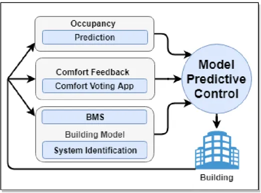
Figure 2.1 depicts a high-level overview of the our system. When the system is installed, occupants within the space are given access to a thermal comfort voting application, which allows each user to vote for their comfort in their working space as frequently as they like. In addition, a wireless network of low-power occupancy sensors are installed overhead to track the distribution of occupants across the space during operation. As the HVAC system runs its control strategy and daily operation occurs in the space, we collect votes from the occupants and track their movement using the overhead sensors. In addition, as the HVAC system runs, we periodically (every 2 minutes) sample the current values of temperature air flow in each zone and the main loop via the BACNet communication protocol, as later explained in Section 5. With this data collected, we have a clear understanding of the recent and current thermal conditions of the space, occupancy distribution, and comfort.
Every 5 minutes, our systems processing pipeline is started, which first retrieves all recent votes, occupancy distribution, and building data samples from the databases where they are stored. With the recent comfort votes from the users across the space, the system chooses the appropriate heating and cooling set points for each zone, such that the occupants will remain comfortable. Using the current distribution of occupants, the system identifies unoccupied or under-occupied zones, candidates for reduced conditioning for energy savings. Using a blended Markov chain [ECC11] trained on historical occupancy data from the running building, the current occu-pancy is sampled from the model to statistically predict the occuoccu-pancy in the near
Figure 3.1: Comfort voting page (left) and feedback (right)
future. Finally, local weather prediction is queried from the public Wunderground API [wun19] to determine expected weather trends.
Finally, we maintain a gray-box thermodynamic model of the building using data-drivensystem identification, which will later be used to predict how the thermal state of the building will respond to a given control sequence. These collected data samples and models are all then used to define, initialize, and solve a model predictive control optimization problem that finds the building actuations minimizing system operation costs subject to occupant comfort constraints based on their voting feedback. These optimized actuations are then communicated with the building and applied for each zone and the main AHU loop. After sufficient time has passed, the processing pipeline will be run again, accounting for any new conditions that have been sensed in the space for future control.
3.1
Human Thermal Comfort
3.1.1 Conditions of the occupant study
To better understand the initial environment and the human factor particularities we run a pre-study survey. This study is approved by the IRB (Institutional Review Board), and the participants were selected to be those who work in the space chosen as the location for our predictive thermal control. The subjects in our study are from a large range of ages from 21 to 60 years old, with a 37% female population from a total of 16 people. From this study we found that 75% of them work between 31 and 40 hours per week from 6AM to 7PM, being exposed to different thermal conditions across the workday. 31.25% have a private office and the rest of them shares a space with few other colleagues. When asked how their thermal preferences compare with their colleagues, 31.25% of the volunteers answered that they prefer a warmer room and 31.25% specified that they prefer a colder room. 56.25% of the people that took this pre-survey answered that they have contacted the facilities team regarding the temperature conditions up to 8 times per person in the last 12 months. 12.50% of them found their thermostat as ineffective and 75% of them do not have a thermostat to control the room temperature. 37.50% of them reported that room temperature enhances their ability to work and 25% believe that it interferes with their ability to work. 37.50% said that they avoided their office because of thermal discomfort and 80% of the total population did clothing adjustment (more or less clothes) when it was necessary. This supports the hypothesis that the thermal comfort has a great impact on the self reported productivity in office spaces, in addition to personal satisfaction. We asked questions related to a new control such as how quickly they would expect their space to be conditioned after adjusting the thermostat and 56.25% answered that they expect to be done in more than 10 minutes. Asking the study’s participants about their satisfaction previous to the new building control, we found that 25% of them felt dissatisfied. With this image in mind, we designed a system to
Figure 3.2: Comfort Voting page in web format
better suit the occupants’ preferences, which thrives in dynamic thermal conditions and is built on a modern infrastructure including open source frameworks.
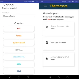
3.1.2 Comfort App Design
To facilitate user interaction with our system, we designed an application in a web for-mat(website) Figure 3.2 distributed to the occupants for iOS and Android platforms, with credentials. It is based on HTML5 and with this feature, content changes in one place are automatically propagated on the mobile phone versions, without passing through the AppStore or Google Play for updates. The app “look and feel” is shown in Figure 3.1. In the left side is the page with the vote buttons whilst in the right side is the page with the green feedback, designed to help the user understand their energy footprint in relatable terms, such as how many hours an electric car could travel or how many hours a building could be powered. Once a vote is issued by a user it is stored in a MySQL database, from where the system incorporates the average vote per zone to find the temperature bounds for that specific zone which will be input
Figure 3.3: Drift strategy setpoints to save energy
into the MPC as constraints.
In our experiments, we allow the bounds to start drifting apart by 1/2◦F every 30 minutes, but remaining between 68 and 76◦F for occupied space and between 55 and 90◦F for unoccupied zone, according to the policies chosen by the building managers. This drift begins when 1 hour has passed since the last issued vote in a zone and makes possible energy savings by allowing the temperature to “float” between these expanding bounds. In normal usage, heating/cooling setpoints are chosen based on occupant voting patterns. However, if these bounds are held unnecessarily tightly, extra energy will be consumed. An example of using drift strategy is shown in Figure 3.3. This figure illustrates that the bounds have started to relax at 12:00 when people go for lunch and in the vote’s absence, at 13:00 they reached the occupied limits (provided by the facility management team) and after 17:00, since the building was empty, the bounds exceeded the previous limits to go closer to the ones for the unoccupied schedule. The zone temperature is not correlated with the bounds values but it is important to remain within the limits. The way the bounds are changing with the drift is retrieved from [WBE16], using the constants mentioned there for the
Figure 3.4: Actuated flow (CFM) as occupancy changes
Fanger formulation (PMV) [Fan70]. In practice, we receive votes from the users that describe how they feel on a scale from cold to hot as in Figure 3.1. By taking the average of all recent votes in the zone as an actual mean vote (AMV) and setting equal to the PMV formulation, we find new bounds values for use in control.
3.2
Occupancy Detection & Prediction
In order to truly condition a building efficiently, it is necessary to be able to reli-ably detect the distribution of occupants throughout the space. A system can save significant energy based on occupancy, as both ventilation and conditioning codes
Figure 3.5: GridEye Sensor before deployment
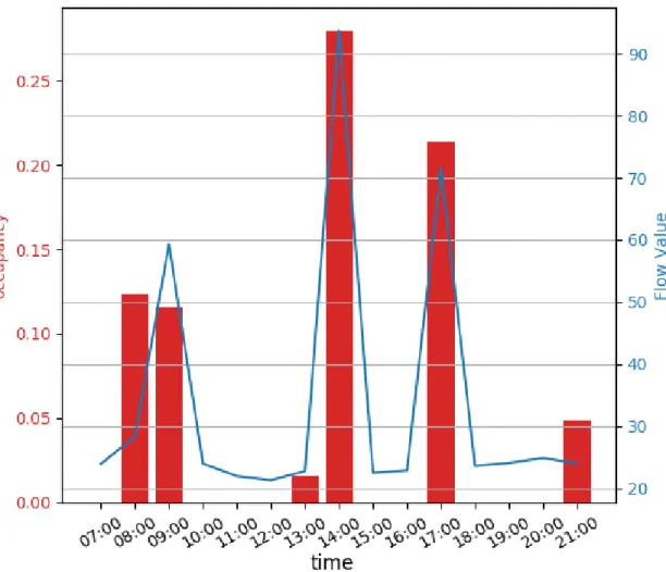
are explicitly defined based on occupancy levels as defined by ASHRAE standards [ASH07b] [ole73]. In an unoccupied zone, ventilation can be set to a minimum level based on the square footage of the zone, and as occupancy increases, ventilation must increase proportionally to prevent buildup of CO2 and other undesired contaminants produced by the occupants as demonstrated in Figure 3.4. We can see in the figure that as the mean occupancy increases, the ventilation tends to closely follow, and that when occupancy goes to zero, ventilation holds steady at a minimum level based on the square footage to be code compliant. Thermal conditioning of the air exhausted into the space, however, changes based on the 0/1 boundary of occupancy. If there are no occupants in the space, the air blown into the zone does not need to be con-ditioned, saving a significant amount of energy. However, if at least one occupant is present, the temperature of the zone must be maintained to keep the occupants comfortable within the space.
For the our system to consider occupancy in its control decisions, we wish to have both occupancy measurement and prediction for the building. For occupancy
mea-Figure 3.6: 8x8 thermal array sensing an occupant
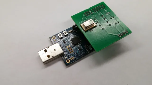
surement, we employ a wireless sensor network of occupancy sensors with Panasonic PIR and Grideye sensors as proposed by [BEC13] and shown in Figure 3.7 and Fig-ure 3.5. The installed devices periodically poll the PIR sensor for recent movement, and if necessary the Grideye captures a thermal image Figure 3.6. Using an expo-nential weighted moving average to maintain a background of the space, background subtraction is used to find active regions in a new frame based on the standard devia-tion of temperature values for each pixel. Then, running an 8-connected components algorithm, we identify the distinct active “blobs” in the frame, which identify the unique heat sources in the frame. As demonstrated in [BEC13], we use a linear re-gressor trained on historical data that maps the size of the largest active blob, the number of blobs, and the number of total active pixels in the image to the predicted number of people in the frame, which we have found to work well in practice. The number of people output by the regressor is then stored in a database to be used later in the processing pipeline.
To allow occupancy prediction, we use a blended markov chain as introduced in [ECC11]. This model is trained with historical data traces of occupancy in this building, and maintains transition matrices for occupancy distribution specific to the time-of-day. This allows our system to query the model with the current distribution of occupants throughout the space and get the predicted future sequence of occu-pancy, with states in the model occurring closest to the current time-of-day being most heavily considered. Since we only consider states observed in the training data as opposed to observable states, there might be states that are not available in a transition matrix for that specific time of day. Suppose we are predicting occupancy for hour Hx. After 3600 steps, we are in some state S, the hours changes from H to Hx, and the model will switch to Hx hourly transition matrix. It is possible the transition matrix for hour Hx for occupancy state S has no probability. This hap-pens when state S never occurs in the Hx training data. Even though in reality the state S can occur in hour Hx, if S does not occur in hour Hx of the training data, then we cannot calculate the transition probabilities for S. This can not be solved by introducing a small probability value of transition to another state as the next selected state may not be represented in the transition matrix as well. The markov chain becomes a random walk until the observed data set captures a particular state. Also, sink state can occur if the next transition matrix does not contain a probabil-ity for the current state. To tackle these issues, rather than considering the closest distance transitions we linearly combine the different transition matrices to obtain blended transition matrix to include all observed states. This increases the number of preferred states available for transition and decreases the chance to select states outside the slot boundaries completely.
Specifically, this type of model will learn time-specific behaviors and sequences, such as occupants morning influx when business hours start, or noontime lunch move-ment. With the ability to predict future occupancy, our system will be able to consider future movement of people and pre-condition the space accordingly.
Figure 3.7: Occupancy sensors before deployment
3.3
System Identification
In optimization, we must consider how the building will react to system inputs such as zone flow and temperature adjustment. As shown in [KMB13b], a resistor-capacitor model can be used to model the thermodynamics of a building where the capaci-tance represents the heat storage capacity of each zone, analogous to room size, and resistance represents how insulated the zones are from each other (i.e. thickness of walls/doors). In this way, we model zone temperature dynamics as follows with model variables enumerated in Table 3.1:
Mn
d
dtTzn = (Tsn−Tzn)cpmzn +Qn+ (To−Tzn)/Rn,o (3.1)
Here, the three terms on the right side represent heat flow from the HVAC system through the vents into the zone, the load due to equipment or machinery, and heat flow from the outside of the building into the zone, respectively. In addition, the Mn term on the left hand side denotes the capacitance of the zone, impacting the
rate at which the zone’s thermal status can be changed. While there may be heat exchangebetweenzones as well, temperature conditions between two indoor zones will
very similar in general, making the heat transfer negligible. In addition, by including these terms, the model becomes highly non-linear, making optimization significantly more difficult.
Before this thermal model can be used, we must estimate values for each zone’s capacity (M), thermal load (Q), and thermal resistance to the outside of the building (R). In practice, the load within each zone and resistance to the outside are difficult to estimate accurately by simply observing the space; factors that contribute to load may be difficult to observe, such as electronic equipment whose heat varies over time depending on usage, appliances in the space that are not constantly running, etc. Similarly, the resistance to the outside of the building is dependent on the insulative abilities of the walls, windows, and doors of the external walls and the area each covers the wall. In contrast, the capacitance of each zone in the building will be directly proportional to the amount of air that can be stored in the zone, which can be determined through most standard floor plans of the indoor space. We note that while this estimate will not consider the space occupied by furniture and people, we consider it a fairly close approximation. In this way, we compute the M values directly, reducing the number of unknown parameters that must be fit from data in the next step.
The remaining parameters, R and Q, are learned periodically using thermal data traces collected within the building. In this way, our model will maintain its relative accuracy over time, as these conditions may be changing based on equipment and personnel usage of the space. To estimate the resistance and load parameters of our system, we use our thermodynamic model of Equation 3.1 and data traces of the system in operation in a least squares analysis to find the values of Q and R that minimize the error of the model given those parameters. This operation is run daily in our system to ensure the model will adapt to changing conditions in the space, such as movement of equipment between zones (printers, computers) or changing working hours of the occupants.
Type Symbol Description
Constants Mn Capacity of a zone
cp Heat capacity of air
Rn,i Resistance between zoneiand zone n
Rn,o Resistance between zonenand outside
ηc, ηh Cooling and heating efficiency
rg Monetary cost of gas per kwh
re Monetary cost of electricity per kwh
τ, N Number of time steps and zones
Tc,min(t) Min cooling temperature
Ts,max(t) Max heating temperature
Ro Required ventilation per occupant
Ran Required ventilation for an area
An Area of a zone
Variable Tzn(t) Zone Temperature
Tsn(t) Supply air temperature to a zone
Tc(t) Cooled air temp from AHU
Tm(t) Mixed Air Temperature
D(t) Damper position for outside air
Tr(t) Return temperature
mzn(t) Mass flow into a zone
ms(t) Total mass flow of all zones
ρu,n(t),ρl,n(t) Upper/lower comfort penalty
φp Penalty coefficient
t, n Time, Zone
Given or To(t) Outside air temperature
Pre-calculated Q Thermal load
On(t) Occupancy
Vmin,n(t) Min ventilation required for a zone
T+
zn(t),T −
zn(t) Upper and lower comfort bounds
As with any process where parameters must be fit to data, it is important that the datapoints used are well-distributed, representing the full data space [Ram69]. In other words, if all datapoints have the same or similar values, a bad parameter fit is likely. For example, if we use temperature values from a conditioned space, the value of load and resistance won’t be reasonable. We use least squares regression to choose the best parameters for our chosen model using the data traces from the building. In our application, during building operation the indoor temperature conditions are relatively constant. For this reason, we require homogeneous distribution of input points on the entire temperature range. We have found that it is best to use data from the mornings when the HVAC system first conditions the space, and nights/weekends when the HVAC system is turned off and the interior temperature drifts due to load and external conditions only.
CHAPTER 4
Model Predictive Control
4.1
Optimization Constraints
To constrain the system, we first must include the thermodynamic model as intro-duced in Equation 3.1:
Constraint 1: Thermal Model of Equation 3.1
The remaining optimization constraints are based on the physical properties of the system, building regulations that the HVAC system must follow, and comfort constraints. In addition, in cases where zone temperatures are outside of comfort ranges as initial conditions for optimization, an upper and lower penalty is added as well to prevent the optimization from becoming infeasible, but guide the zone temperature into a comfortable range as quickly as possible.
Constraint 2: Tc(t) ≤ Tm(t) – The cooling coil can only cool the air received from
the economizer.
Constraint 3: Tc(t)≥Tc,max – Cooling capacity of cooling coil.
Constraint 4: Ts(t)≥ Tc(t) – Heating coils can only increase the temperature of the
air supplied by the AHU.
Constraint 5: Ts(t)≤Ts,max – Max capacity of heating coil.
Constraint 6: mzn(t) ≥Vmin,n(t) – The zone’s minimum ventilation required for
Constraint 7: mzn(t)≤mmaxn – The VAV’s maximum ventilation capacity.
Constraint 8: 0≤D(t)≤1 – Physical damper constraint.
Constraint 9: D(t)≥Dmin – Minimum outside air requirement. Constraint 10:
N
P
n=1
mzn(t)≤AHUmax – The fan’s maximum ventilation capacity.
Constraint 11: ρun(t) +T
+
zn ≥Tzn(t)≥T
−
zn−ρun(t) – Comfort bound
Constraint 12: ρun(t)≥0, ρln(t)≥0 – Penalty functions can only increase cost
By honoring these system constraints, the model predictive control will respect the requirements and limitations of the physical HVAC system when considering potential actuations.
4.2
Objective function
To choose the best actuation sequences possible, we create the objective function such that the cost of system operation is minimized. In our HVAC system, the three primary energy consumers are AHU ventilation and cooling (both electricity) and heating (gas). While there are further consumers such as water pumps for heating and cooling, these are more minor consumers, and are not considered in our model. Similarly to the thermodynamic model previously presented in Section 3.3, we can use the temperature values before and after heating and cooling to compute the amount of energy that has been transferred. For instance, we can compute the energy used for cooling at times t ∈1. . . τ as
Pc = cp ηc τ X t=1 ms(t)(Tm(t)−Tc(t)) (4.1)
whereTm(t) is the warmer mixed air,Tc(t) is the cooler output,ms(t) is the mass flow
rate,cp is the heat capacity of air, andηcis the efficiency of the air conditioner. With
defined in Table 3.1, this equation will provide the kWh consumed in heating, which can then be multiplied into the cost of electricity re to convert to monetary value.
The mixed air temperature Tm is a mixture of the return temperature Tr and the
outside temperature (To), the ratio of which is controlled by the economizer damper
position D(t). At D(t) = 1, 100% of the mixed air is recirculated, and at D(t) = 0, 100% of the air comes from the outside.
Tm(t) = D(t)Tr(t) + (1−D(t))To(t) (4.2)
While fresh air is required to prevent buildup of gases in the space, more re-circulation allows the system to save energy, as the re-circulated air has already been conditioned to roughly the desired temperature. The return temperature, then, is a mixture of outgoing air temperature from each zone, weighted by that zone’s mass air flow:
Tr(t) = N P n=1 mzn(t)Tzn(t) ms(t) (4.3) The technique to measure energy consumed for heating is similar to that of cooling. We consider the temperature increase across the heating coil in each zone and the mass flow of air to get
Ph = cp ηh N X i=1 τ X t=1 mzi(t)(Tsi(t)−Tc(t)) (4.4)
where mzi is the mass flow for zone i, Tsi is zone i’s supply temperature into the
room, andTc(t) is the cool air temperature in the main loop. Finally, we consider the
cost of the fan, which was found to be a squared increase with respect to mass flow in [KMB13b] with an efficiency factor of ηf:
Pf = τ
X
t=1
ηfms(t)2 (4.5)
Considering the differing costs for gas and electricity, the minimization problem can be written as follows where re and rg are the dollar costs per kWh for electricity
.108 $/kWh for electricity. In our deployment, this means the optimized actuations will prefer to provide more gas heating due to the cheaper costs, but under different pricing conditions OFFICE will find the appropriate control that will minimize costs for any pricing.
min
mn(t),Tzn(t),Tsn(t),Tc(t),D(t)
t∈1...τ,n∈1...N
re(Pc+Pf) +rg(Ph) +Cs
subject to: Constraints 1-12
(4.6)
As the objective function and constraints are nonlinear with respect to the optimiza-tion variables, the optimizaoptimiza-tion problem as written is non-convex which may cause the optimized solutions to be local and not global optima. Future work may consider the process of model linearization, but analysis must be done to ensure model accuracy is not substantially reduced. In practice, our system models the thermodynamics of the 8 zones of our test building (N = 8) 1 hour into the future, at 10 minute inter-vals (τ = 6). Despite model non-convexity, a solution is found in seconds using the Julia [BEK14] optimization framework’s IPOPT solver for our test building.
When optimization is finished, it returns the optimal setpoints of discharge tem-perature and mass flow for each VAV in the system, damper position in the econo-mizer, and temperature setpoint for cooling in the AHU for the next hour into the future at 10 minute intervals. In addition, for each of these discrete timesteps, the optimization provides the state of the system subject to the optimal control, as pre-dicted by the thermodynamic model. In practice, although optimization considers the evolution of the system for a time window of 1 hour into the future, when opti-mization is finished only the first set of actuations (i.e. actuations at t = 0) are sent to the building for actuation. Then, 10 minutes in the future, all data is queried and optimization is completed again to correct for any error in prediction that may have occurred.
CHAPTER 5
System Implementation
Our system has several modules that require data gathering capabilities, as discussed in Sections 5 and 4. In this section we explain the building interaction with various modules that form this system, and practical considerations in its design. Figure 5.1 provides a detailed view of the system architecture, along with the backbone storage systems that maintain the large amount of data required in processing. Due to the different types of data we maintain for our processing pipeline, we maintain two distinct databases; for data sources that are periodic such as building sensor data, a time-series data called Influx [inf13] is used, and for data that is not time-series is stored in a relational MySQL [MyS95] database.
Building control is not easy. Incorrect actuation commands can result in discom-fort to the occupants in the space, reduction of hardware lifetime through an unex-pectedly high number of physical cycles, or even direct damage of HVAC equipment. This is especially risky due to the reliance of the system on high data quality from the various data sources in the space. In our experience, it is common for embedded sensors within the building equipment to become miscalibrated or simply fail, and similarly we have found actuators that will not obey a request to change states. For these reasons, the highly modularized structure of our system has been instrumental to maintaining a high quality of control. To ensure system operation, a number of fail safes have been implemented; features within the Influx time-series database have allowed us to create custom alarms to sense when sensors have not provided data for a period of time, allowing us to detect and correct issues in our deployments, and
Figure 5.1: OFFICE System Architecture
modules in the processing pipeline add a layer of redundancy on actuation requests to ensure our model predictive control output can never exceed pre-defined minimum and maximum values for control.
The Influx database manages real-time data arriving from periodic data sources. Sensor data is collected by the Building Management System (BMS) periodically throughout the day (every 2 minutes). This sensor data is gathered from sensors such as flow and temperature sensors throughout the HVAC system. While the BMS collects high-resolution data of all points, limitations in the WebCTRL system cause it to severely slow down when third-party applications fetch this data in bulk. As this is a critical system to the facilities management crews on campus, we circum-vent this limitation by fetching this data directly from the devices themselves using a data communication protocol for Building Automation and Control Networks called BACnet [LHM12], and stored in the Influx time series database. In addition, the dis-tributed network of occupancy sensors introduced in Section 3.2 periodically sample and transmit occupancy data to a network-enabled border router in the space, where
it is relayed to Influx as well. In contrast, the relational MySQL database manages non-periodic data. For instance, as the thermal comfort application introduced in Section 3.1 receives votes from the users, they are recorded and stored in MySQL to maintain the source of the vote, associated zone for conditioning, etc. To facili-tate easy use of this database, the comfort voting application has WEB and Mobile applications built on top of Django(Python) with better support for MySQL.
The time-series database is critical after optimization as well. When the model predictive control finds an optimal solution, it provides a set of setpoints that must be conveyed to the building, and these actuations are all stored in Influx. Once the actuations are validated, a separate module fetches these points from influx and initiates communication with the building. Although the actuations can be set via the Bacnet protocol directly to the actuators in the system, this will cause issues when WebCTRL tries to overwrite the setpoints using its own strategy. Instead, our system communicates with the WebCTRL service’s SOAP API as a middleman and overwrites the WebCTRL setpoints, which prevents the interference of the WebCTRL control strategy and allows the facilities techs familiar with the WebCTRL system to have full visibility of the control decisions of the OFFICE system.
As building actuation is done on the scale of minutes, the time it takes to solve for a single optimization problem is less than 5 seconds. Once the optimizer solves the problem, a set of control inputs is obtained, such as the mass flow, discharge tempera-ture, damper positions and supply temperature which is saved in Influx database. The predicted values as explained in section [4] are also saved in the same database.Once everything is in place, we run an actuation script every 5 minutes to read the actu-ation points from database and these control set points are then transmitted to the BMS using BMS’s SOAP based API, which then uses its own built-in PID loops to achieve the set points passed to the building’s equipment.
An example of how we control would be setting the point for the mass flow. Our solution contains the flow for each zone which can then be set as required mass flow
Figure 5.2: OFFICE Grafana Node Map
via the BMS. We only adjust the set-point, and the building is capable of changing the supply fan’s speed and damper position for each zone to meet the needs of all the zones. Every actuation period the points we set include all zones’ mass flow, zones’ supply temperature, discharge temperature at building level. In order to utilize the return air from HVAC system we modify the outside air damper position which help us to conserve energy as the amount of air that needs to be reheated reduces and less energy is spent on reheating the air going in.
Integration with the actual BMS is done in a such way that if the facility manage-ment team would like to take control over, it is possible to make an instantly switch from our strategy to the BMS control strategy. As a final layer of oversight, the OFFICE system features monitoring and dashboarding visualization to be used by the facilities techs. We used Grafana [Gra14] and a web application build on NodeJS to integrate a visual monitoring and dashboaring system with our Influx Database to keep track of active wireless sensors for occupancy detection, as well as email alerts in case of a failures, or if a certain zone is not behaving as expected, etc. Figure 5.2
Figure 5.3: OFFICE Zone Temperature Plots
gives an overall picture of the mean number of occupants in a particular room based on a mote and Figure 5.3 provide a historical picture of zone temperature of all the zone. In case a zone temperature goes beyond set bounds, the team gets an email notification with a a visual notification on the dashboard.
In the case that the OFFICE system does something incorrect, we provide the facilities techs with a “kill switch” that immediately terminates OFFICE control and returns to the WebCTRL strategy. To date this feature has not been used.
CHAPTER 6
Case Study
6.1
Environmental Conditions
To perform a comparison of our system against state-of-the-art building control, it is deployed in a LEED Gold certified building housing the facilities management crew and various administrative staff of our university Figure 6.1. The region within the building under our control is approximately 5000 square feet, and is controlled by 1 air handler unit divided into 8 zones, each provided by a variable air volume (VAV) unit. The HVAC system is controlled by a WebCTRL building management system. In total, the zones cover 4 offices, around 20 cubicles, a conference room, a break room, and an open hallway occupied by two receptionist desks, with each type having its own pattern of usage.
As the university is maintained by the department of facilities and its occupants, our occupants have abnormal hours. Maintenance personnel arrive as early as 5 am and cleaning staff frequently use the building until midnight. In all, there are 18 full-time staff members and several part-time student workers in the building, with more coming in and out as a central operating base. The system was evaluated for a total of 4 weeks ; as the building management system is inactive on weekends, our system analysis includes 20 days of operation on weekdays.
Figure 6.1: 3-D Model of building
6.2
Performance Metrics
To determine the merit of the our system, we launch it in our building for 20 days, and compare its operation with the baseline WebCTRL strategy with respect to several metrics. In practice, it is infeasible to run the two control strategies at the same time, so it is difficult to compare them under identical conditions; for instance, the outdoor weather changes daily, so the control sequences will change as well. To make sure we have as fair a comparison as possible, for each day of operation under the system, we take the day’s 24-hour outdoor temperature profile, and compare it to our data under WebCTRL operation. When we find the WebCTRL day with the most similar temperature trend, we use it to compare to our system operation. We note that in some cases, more than one day may map to the same WebCTRL day, leading to repeated trends for analysis in WebCTRL data.
The primary purpose of the building management system is to make the indoor en-vironment comfortable for the building occupants. To compare comfort under the two systems, we perform a pre and post-study survey with each occupant in the building to understand how their thermal conditions are under the existing baseline strategy,
Figure 6.2: Temperature prediction versus ground truth
and how they change under the control of our system. This provides us the clearest view into the comfort provided by the system to this building’s occupants. In addi-tion, to provide a more quantitative analysis on the more general populaaddi-tion, we use Fanger’s formula for PMV [Fan70] to estimate comfortable temperature bounds for the “standard” occupant within the current seasonal conditions. With these bounds in mind, we can step through all data from a system’s operation, and any time the zone temperature goes outside the bounds, we add the distance from the bound to a sum.By conducting this analysis on both systems, we can directly compare how well in the more general sense the two systems can maintain comfortable conditions.
Figure 6.3: Model error characteristics for each zone
control strategy costs as little money and consumes as little energy as possible. Al-though minimizing system operational costs and consumed energy are not equivalent goals, we wish to reduce both energy consumption and costs in comparison to the baseline strategies. While we do not have access to direct measurement of energy con-sumption or costs in the running system, we can use the energy and cost equations derived in Section 4.2 to compute the energy consumed in heating, cooling, and AHU fan using the data trends from the OFFICE system and its most similar weather day under the WebCTRL strategy. While these equations describe the “ideal” energy transfer in the system and will not include energy losses due to heat dissipation or other inevitable sources of loss, it provides us the ability to compare these systems in exactly the same way for comparison.
6.3
Model Accuracy
As our system runs its control within the test building, the model predictive con-trol framework is optimizing concon-trol actuations based on the model describing the
Figure 6.4: Zone 1: Temperature prediction versus ground truth
expected building reaction. To determine whether the thermodynamic model is cap-turing the effects within the building, we can compare MPC’s predicted temperature at time t = +10m to the ground truth temperature that actually occurred at time t= +10m. For instance, Figure 6.2 demonstrates the ground truth zone temperature in Zone 5, against the temperature predicted by the model 10 minutes earlier. We can see in this specific example that the predicted values closely follow the true ones, but that at some times (i.e. 07:00) the model predicts temperatures to increase too quickly, or others (i.e. 19:00) the model predicts the temperature will decrease too quickly.
future conditions, the distribution of errors across our 20 days of deployment is shown for each zone in the system in Figure 6.3. In this figure, the center line within each box is the median error for that zone, the upper and lower ends of the boxes define quartiles 1 and 3, the whiskers denote extreme data not considered outliers, and the crosses represent outliers. We can see here that with the exception of zones 1 and 3, the median error for all zones is below 1 degree Fahrenheit, with outliers exceeding 2 degrees. While we believe this is reasonable performance in the more general case, it is clear that the model had difficulty making accurate predictions for zones 1 and 3. Zone 1 is a break room in the building, and has many characteristics that make prediction difficult. As a break room, occupancy patterns were found to be very sporadic and appliances (1 fridge, 2 vending machines, 1 printer) cause irregular thermal load in the room that was difficult to model. Zone 1’s error in prediction can be seen in Figure 6.4. Zone 3, an open cubicle area, had the main door to the outside, which resulted in a large influx of outside air every time somebody entered or exited the building. It is important to note that while some zones have higher modeling error, the OFFICE framework will be able to provide control as long as the model predicts future states in the direction of the ground truth. In these cases, OFFICE’s periodic re-solve of control optimization with corrected initial conditions will guide the solution towards the desired state, even if it is sub-optimal w.r.t. cost. To demonstrate this point, Section 7 will show that the OFFICE system is capable of improved occupant comfort and energy savings despite this challenge in modelling.
CHAPTER 7
Results
For our analysis, we want to compare the state-of-art building control that is op-erational in the top of the line green buildings with our OFFICE control strategy. We think this is valid baseline comparison as this represents the best strategy that is implemented in current top quality building stock in the U.S. As mentioned in Section 6.2, we are interested in comparing both the quality of thermal comfort and the energy use/cost results between the two systems.
7.1
Thermal Comfort Analysis
Table 7.1 shows the results from the pre-survey and the post-survey. The first thing to notice is that the satisfaction level in the pre-survey for the WebCTRL baseline strategy is very good. Only 25% of users are dissatisfied, with 50% of all users being satisfied or somewhat satisfied. Previous work has shown that the percentage of users
Satisfaction level Pre-survey Post-survey Satisfied or very satisfied 25.0% 30.0%
Somewhat satisfied 25.0% 50.0%
Neutral 25.0% 20.0%
Somewhat dissatisfied 18.75 % 0.0%
Dissatisfied 6.25% 0.0%
Figure 7.1: Example of thermal comfort for all zones in WebCTRL
Total Sum No of Days Average
WebCTRL 3543.3 84 42.2
OFFICE 459.8 20 23.0
Table 7.2: Quality of Thermal Comfort
dissatisfied was in general much larger, varying from 50% to 75% [EC12, WBE16]. This is not completely surprising though, as the building went through LEED Gold certification process and two very experienced HVAC engineer tuned up the control routines in the building to make them as efficient as possible, debugging comfort issues with users in the process. In the post-survey column, we see the results of the post-survey after running the OFFICE system. The level of dissatisfaction is zero percent, and 80% of the users were satisfied or somewhat satisfied, with the remaining 20% being neutral.
of thermal comfort than OFFICE. Figure 7.1 shows an example of thermal comfort for all the zones when running WebCtrl for a single day. As mentioned in Section 6.2, we use Fanger’s formula for the Predictive Mean Vote (PMV) [Fan70] to estimate com-fortable temperature bounds for the “standard” occupant within the current seasonal conditions, as defined by ASHRAE standard 55 [ASH07a]. Office-like environments do not require special thermal needs, so they are considered Class C environments according to the classification scheme included in ISO 7730 [Iso05]. The maximum high/low end of the comfort range for Class C environments has PMV values of +/-0.7, which we determined to be a temperature range between 70◦F and 76◦F. From Figure 7.1 we see that over the course of the day, many zones get close to the the tem-perature limits, and specifically zones 1 and 3 exceeds the low and high limits several times during the day. The figure shows clearly that WebCTRL exceeds the comfort temperature bounds and would tend to provide poor quality of thermal comfort to its occupants. In order to provide more quantitative results over the course of many more days, we step through all data from both WebCTRL and OFFICE, and any time the zone temperature goes outside the bounds, we add the distance from the bound to sum, i.e. we calculate the L1 distance when bounds are exceeded. The results are shown in Table 7.3. From the table, we see that WebCTRL produces a significantly larger distance when comfort bounds are violated, with an average distance across all zones of 42.2/day versus OFFICE 23.0/day, an 83.5% decrease in quality of comfort by WebCTRL compared to OFFICE.
Figure 7.2 shows the thermal preferences vote distribution for all the users in our building. We see that ∼41% of all the users’ votes were on the hot/warm side of the scale, with ∼32% of all the users’ votes on the cold/cool side, and ∼27% of all users’ vote being neutral. This figure provides an indication that temperatures might be on the warmer side for the majority of the zones. To verify this intuition based on the users thermal preferences, we plot in Figure 7.3 the zone average temperature variation from all zones across different times of the day for a sample experimental day.
Figure 7.2: Thermal preferences vote distribution for the users in our building. Values [-3,-2,-1,0,1,2,3] corresponds to [Cold, Cool, Slightly Cool, Neutral, Slightly Warm, Warm, Hot] in our comfort app.