econstor
www.econstor.eu
Der Open-Access-Publikationsserver der ZBW – Leibniz-Informationszentrum Wirtschaft
The Open Access Publication Server of the ZBW – Leibniz Information Centre for Economics
Standard-Nutzungsbedingungen:
Die Dokumente auf EconStor dürfen zu eigenen wissenschaftlichen Zwecken und zum Privatgebrauch gespeichert und kopiert werden. Sie dürfen die Dokumente nicht für öffentliche oder kommerzielle Zwecke vervielfältigen, öffentlich ausstellen, öffentlich zugänglich machen, vertreiben oder anderweitig nutzen.
Sofern die Verfasser die Dokumente unter Open-Content-Lizenzen (insbesondere CC-Lizenzen) zur Verfügung gestellt haben sollten, gelten abweichend von diesen Nutzungsbedingungen die in der dort genannten Lizenz gewährten Nutzungsrechte.
Terms of use:
Documents in EconStor may be saved and copied for your personal and scholarly purposes.
You are not to copy documents for public or commercial purposes, to exhibit the documents publicly, to make them publicly available on the internet, or to distribute or otherwise use the documents in public.
If the documents have been made available under an Open Content Licence (especially Creative Commons Licences), you may exercise further usage rights as specified in the indicated licence.
zbw
Koopman, Siem Jan; Nguyen, Thuy Minh
Working Paper
Fast Efficient Importance Sampling by State Space
Methods
Tinbergen Institute Discussion Paper, No. 12-008/4
Provided in Cooperation with:
Tinbergen Institute, Amsterdam and Rotterdam
Suggested Citation: Koopman, Siem Jan; Nguyen, Thuy Minh (2012) : Fast Efficient Importance Sampling by State Space Methods, Tinbergen Institute Discussion Paper, No. 12-008/4, http:// nbn-resolving.de/urn:NBN:nl:ui:31-1871/38495
This Version is available at: http://hdl.handle.net/10419/87536
TI 2012-008/4
Tinbergen Institute Discussion Paper
Fast Efficient Importance Sampling by
State Space Methods
Siem Jan Koopman
1Thuy Minh Nguyen
21 Faculty of Economics and Business Administration, VU University Amsterdam, and
Tinbergen Institute;
Tinbergen Institute is the graduate school and research institute in economics of Erasmus University Rotterdam, the University of Amsterdam and VU University Amsterdam.
More TI discussion papers can be downloaded at http://www.tinbergen.nl
Tinbergen Institute has two locations: Tinbergen Institute Amsterdam Gustav Mahlerplein 117 1082 MS Amsterdam The Netherlands Tel.: +31(0)20 525 1600 Tinbergen Institute Rotterdam Burg. Oudlaan 50
3062 PA Rotterdam The Netherlands Tel.: +31(0)10 408 8900 Fax: +31(0)10 408 9031
Duisenberg school of finance is a collaboration of the Dutch financial sector and universities, with the ambition to support innovative research and offer top quality academic education in core areas of finance.
DSF research papers can be downloaded at: http://www.dsf.nl/
Duisenberg school of finance Gustav Mahlerplein 117 1082 MS Amsterdam The Netherlands Tel.: +31(0)20 525 8579
Fast Efficient Importance Sampling
by State Space Methods
Siem Jan Koopman
(a,b)Thuy Minh Nguyen
(c)(a) Department of Econometrics, VU University Amsterdam (b) Tinbergen Institute
(c) Deutsche Bank, London
January 30, 2012
Some keywords: Kalman filter; Monte Carlo maximum likelihood; Simulation smoothing.
JEL classification: C32, C51.
Acknowledgements: We would like to thank Andr´e Lucas and Marcel Scharth for giving comments on an earlier version of this paper. The usual disclaimer applies.
Address of correspondence: S.J. Koopman, Department of Econometrics, VU University Amsterdam, De Boelelaan 1105, NL-1081 HV Amsterdam, The Netherlands.
Fast Efficient Importance Sampling by State Space Methods
Siem Jan Koopman and Thuy Minh Nguyen
Abstract
We show that efficient importance sampling for nonlinear non-Gaussian state space models can be implemented by computationally efficient Kalman filter and smoothing methods. The result provides some new insights but it primarily leads to a simple and fast method for efficient importance sampling. A simulation study and empirical illustration provide some evidence of the computational gains.
1
Introduction
For the modeling of an observed time seriesy1, . . . , yn, we consider a parametric model that
we formulate conditionally on a time-varying parameter vector θt. The conditional model
for the observations is given by
yt|θt∼p(yt|θt;ψ), t= 1, . . . , n, (1)
where ψ is a fixed parameter vector, with observation density p(yt|θt;ψ) that is possibly
non-Gaussian and may represent a nonlinear relation between yt and θt. Conditional on θ1, . . . , θn, the observationsy1, . . . , ynare serially independent. The time-varying parameters
inθtcan represent different features of the model including constant, variance and regression
coefficients. Different dynamic specifications for the parameters inθt can be adopted. In our
analysis, the conditional observation density and the dynamic model forθt must be specified
but both may depend on the fixed parameter vector ψ.
When (i) the conditional observation density is Gaussian, (ii) the relation betweenytand θt is linear and (iii) the dynamic model for θt is linear Gaussian, our time series modelling
framework reduces to the linear Gaussian state space model as discussed, for example, in Durbin and Koopman (2001, Part I). In this framework, we can rely on the celebrated Kalman filter and its related smoothing method for the signal extraction ofθt, the maximum
likelihood estimation of ψ and the forecasting of yt. However, when we depart from one of
the three assumptions, these analyses cannot be carried out using the Kalman filter. We then rely on numerical methods to evaluate the high-dimensional integrals that are required for such analyses. In this paper we discuss Monte Carlo estimation based on importance sampling methods.
The general ideas of importance sampling are established in statistics and econometrics, see Kloek and Van Dijk (1978), Ripley (1987), and Geweke (1989). Importance sampling techniques for state space models have been explored by Danielsson and Richard (1993), Shephard and Pitt (1997), Durbin and Koopman (1997), So (2003) and Jungbacker and Koopman (2007). A textbook treatment is given by Durbin and Koopman (2001). The performance of this approach to Monte Carlo estimation relies on the successful construction of an importance density. Several methods for designing an importance density for time series modelling have been proposed. For example, Shephard and Pitt (1997) and Durbin and Koopman (1997) adopt an importance density based on the mode of the conditional density.
In this paper we consider the efficient importance sampling (EIS) method of Liesenfeld and Richard (2003) and Richard and Zhang (2007) where the sampling is based on a global approximation of the original model. We show that EIS can be implemented using standard Kalman filter methods. It leads to a simple and fast procedure for importance sampling. We discuss how the resulting EIS procedure is related to the procedure of Shephard and Pitt (1997) and Durbin and Koopman (1997), hereafter referred to as SPDK. A simulation study provides the evidence of the computational efficiency gains.
The remainder of the paper is organized as follows. In Section 2 we review the EIS and SPDK methods for constructing the importance density for nonlinear non-Gaussian state space models. In Section 3 we show how the EIS method can be implemented using state space methods and illustrate the gains of our modified efficient importance sampling method by a simulation study. In Section 4, details are provided for an effective implementation of the method. In Section 5, the method is applied to a time-varying model for counts in a simulation study and a stochastic volatility model for daily returns of pound/dollar exchange rates in an empirical study.
2
The model
The dynamic model specification under consideration is given by the observation density
p(yt|θt;ψ) as introduced in (1) and with the stochastically time-varying parameter vector θt
specified as
θt=Zt(αt), t= 1, . . . , n, (2)
whereZt(·) is a fixed known function that may depend on the parameter vectorψ and where αt is the stochastically time-varying state vector. The linear Gaussian dynamic process for
αt is given by
αt+1 =Ttαt+Rtηt, ηt∼NID(0, Qt), α1 ∼N(0, Q0), (3)
where the elements of the matrices Tt and Rt and the variance matrices Qt and Q0 are
known except that some elements have a possible dependence on parameter vectorψ, fort = 1, . . . , n. The disturbances ηt are normally independently distributed, serially uncorrelated
and are not dependent on the normally distributed initial state vectorα1. All stochastic and
non-stochastic variables have appropriate dimensions and they will be given only when it is necessary. The observation yt is typically a scalar but the methods presented in Section 3
are also applicable for a vector of observationsyt. Illustrations of special cases of our general
modelling framework are given below.
Signal plus heavy-tailed error model
When the time series observations yt are randomly contaminated by noise with with large
shocks, we may wish to remove the noise from the signal and to model the noise explicitly by a heavy-tailed density. We then may consider the model
yt=θt+εt, εt∼τ(0, σ2, ν), t = 1, . . . , n, (4)
where τ(µ, σ2, ν) refers to the Student’s t density with mean µ, variance σ2 and degrees of
freedom ν. The dynamic specification for θt can be determined by (2) and (3). The model
clearly fits in our general framework with p(yt|θt;ψ) =τ(θt, σ2, ν) in (1).
Stochastic volatility model
A time series of financial returns is mostly subject to clusters of volatility changes which can effectively be modelled by a dynamic processes for the variance. A basic version of the stochastic volatility model for a time series of returns yt is given by
yt =µ+ exp(
1
2θt)εt, εt∼NID(0, σ
2), t= 1, . . . , n, (5)
where µ is a constant and εt is normally distributed with zero mean and variance σ2. The
dynamic specification forθt can be determined by (2) and (3). The conditional observation
density (1) is given by p(yt|θt;ψ) = − 1 2log(2π σ 2)− 1 2θt− 1 2σ2 exp(−θt)(yt−µ) 2, t = 1, . . . , n.
The stochastic volatility model can be extended in many ways. For example, the Gaussian density for εt can be replaced by the Student’s t density as in (4); we refer to Shephard
(2005) for extensive discussions on stochastic volatility models.
Time-varying model for counts
Time series of counts can be modelled by the Poisson density with the intensity parameter as a function of the time-varying signalθt that we can specify as (2) and (3). The observation
density is then given by
p(yt|θt;ψ) =ytlogθt−θt−log(yt!), t= 1, . . . , n. (6)
Other densities from the exponential family can also be considered such as the Binomial density. More examples are documented in Durbin and Koopman (2001, Chapter 10).
3
Efficient importance sampling
We discuss our implementation of the efficient importance sampling (EIS) method by con-sidering likelihood evaluation. In the next section we discuss other applications in which EIS plays an important role including signal extraction, maximum likelihood estimation of
ψ and forecasting of future observations yt.
The likelihood function of the model (1), (2) and (3) for the observed vector y = (y′
1, . . . , yn′)′ and as a function of parameter vectorψ can be represented by
L(y;ψ) = Z p(y, α;ψ) dα= Z p(y|α;ψ)p(α;ψ) dα, (7) whereα= (α′
1, . . . , α′n)′. This expression may suggest a basic Monte Carlo evaluation of the
likelihood function via
b L(y;ψ) = M X i=1 p(y|α(i);ψ), α(i) ∼p(α;ψ), (8)
where α(i) refers to the ith simulated sample of α that is generated from the unconditional
density p(α;ψ) with i = 1, . . . , M. The standard law of large numbers (LLN) insists that
b
L(y;ψ) converges toL(y;ψ) asM → ∞. However, since the simulation ofαhas no reference to the data vectory, the efficiency of the estimate will be very low and therefore we need an extremely large value of M. Numerical evaluation of (7) is also not feasible given the high
dimensional vector α.
Given the serial independence properties for the observations yt conditional onθt and for
the disturbances ηt, we have
L(y;ψ) = Z "Yn t=1 p(yt|αt;ψ)p(αt|αt−1;ψ) # dα, (9)
with p(α1|α0;ψ) =p(α1;ψ) and where p(yt|αt;ψ) =p(yt|θt;ψ) given the signal specification
(2). We also have p(αt|αt−1;ψ) =p(ηt−1;ψ) = NID(0, Qt−1) for t= 1, . . . , n.
3.1
Importance density
The numerical evaluation of (9) becomes feasible when using Monte Carlo methods and we consider the method of importance sampling; see Ripley (1987) for an introduction to simulation methods. For the purpose of evaluating (9) via importance sampling, we introduce the importance density based on the linear Gaussian joint density g(y, α;ψ) with properly defined mean vector and variance matrix. Its dependence onψis derivative from the original model (1) – (3). The decomposition g(y, α;ψ) = g(y|α;ψ)g(α;ψ) is valid and we assume that g(y|α;ψ) = n Y t=1 g(yt|θt;ψ), g(α;ψ) =p(α;ψ) = n Y t=1 p(αt|αt−1;ψ),
since g(yt|αt;ψ) = g(yt|θt;ψ) from (2) and where p(αt|αt−1;ψ) = NID(0, Qt−1), for t =
1, . . . , n. Since the dynamic specification for the state vector in (3) is linear Gaussian, we adopt the same state specification for the importance density. The Gaussian observation density is expressed by g(yt|θt;ψ) = exp at+b′tθt− 1 2θ ′ tCtθt , t= 1, . . . , n, (10)
where zt = zt(yt;ψ) is a known function of yt and ψ for z = a, b, C and t = 1, . . . , n. The
constant at is needed to ensure that g(yt|θt;ψ) integrates to one. The key functions are bt and Ct which determine the mean and variance of the density g(yt|θt;ψ). An effective
importance sampler is obtained by selecting appropriate values forbtandCtfort= 1, . . . , n.
Hence the design of the importance sampler is elegantly reduced to a choice forbt and Ct.
We notice that the importance density can also be expressed in terms of the constructed variable xt=Ct−1bt and the linear Gaussian model
where the Gaussian disturbances u1, . . . , un are serially uncorrelated. We can show that the
conditional obervation density function (10) is equivalent tog(xt|θt;ψ); in logs, we have
logg(xt|θt;ψ) = − 1 2log 2π− 1 2log|Ct| − 1 2 (xt−θt)′Ct−1(xt−θt) = at+b′tθt− 1 2θ ′ tCtθt,
sincext=Ct−1bt, whereatcollects all terms that are not associated withθt. Hence it follows
immediately that g(y|α;ψ)≡ n Y t=1 g(xt|θt;ψ),
when we assume that xt is modelled by (11) for t = 1, . . . , n.
3.2
Likelihood evaluation via importance sampling
The actual importance density for the evaluation of (7) is chosen as
g(α|y;ψ) =g(y|θ;ψ)g(α;ψ)/ g(y;ψ),
where g(α;ψ) = p(α;ψ). The likelihood function (7) with the importance sampling density incorporated is given by
L(y;ψ) =
Z p(y|α;ψ)p(α;ψ)
g(α|y;ψ) g(α|y;ψ) dα.
After some minor manipulations, we can express the likelihood function as
L(y;ψ) =g(y;ψ) Z "Yn t=1 w(yt, αt;ψ) # g(α|y;ψ) dα, w(yt, αt;ψ) = p(yt|αt;ψ) g(yt|αt;ψ) , (12)
where w(yt, αt;ψ) is referred to as the importance weight, fort = 1, . . . , n.
The evaluation of the likelihood function by means of importance sampling takes place by simulating state vectors from the importance density g(α|y;ψ) which we denote by
α(i)=α(i)′
1 , . . . , α(ni)′
′
∼g(α|y;ψ), i= 1, . . . , N.
Since we can represent g(y, α;ψ) by the linear Gaussian state space model (11), (2) and (3), we can simulate α from the smooth density g(y, α;ψ) via the simulation smoothing method; see, for example, Fruhwirth-Schnatter (1994), Carter and Kohn (1994), de Jong
and Shephard (1995) and Durbin and Koopman (2002). Given the simulated realisations
α(i), fori= 1, . . . , N, the likelihood function is computed by
b L(y;ψ) =g(y;ψ)M−1 N X i=1 n Y t=1 wit, wit =w(yt, α (i) t ;ψ). (13)
Some practical guidance for the computation ofLb(y;ψ) for the purpose of parameter estima-tion is given in Secestima-tion 4.1. We expect that the Monte Carlo estimate (13) is more efficient than the estimate (8) since we simulate αt(i) with a reference to the data vector y.
3.3
Efficient importance sampling
The values forbt and Ct, with t = 1, . . . , n, need to be determined before the calculation of
(13) can start. Here we follow Richard and Zhang (2007) and adopt their efficient importance sampling (EIS) method. They propose to choose bt and Ct such that the criterion
It=
Z
λ2t(yt, αt;ψ)p(yt, αt;ψ) dαt, λt(yt, αt;ψ) = logw(yt, θt;ψ)−λ,¯ (14)
is minimized for each t separately and where ¯λ is the normalizing constant such that the expectation of λt with respect to the true model p(yt, αt;ψ) is zero. We therefore interpret It as the variance of the logged importance weight function with respect to p(yt, αt;ψ). We
notice that the variablesbt and Ct determineg(yt|θt;ψ) that is part of w(yt, θt;ψ) and hence
of λt(yt, αt;ψ). The functionIt cannot be evaluated analytically for the same reason as the
likelihood function (7) cannot be evaluated analytically. Hence we follow the same approach of introducing the importance densityg(αt|y;ψ). The criterion to be minimized can then be expressed as It = Z λ2t(yt, αt;ψ) p(yt, αt;ψ) g(αt|y;ψ)g(αt|y;ψ) dαt ∝ Z λ2t(yt, αt;ψ) p(yt|αt;ψ) g(yt|αt;ψ) g(αt|y;ψ) dαt ∝ I∗ t, where I∗ t = Z λ2t(yt, αt;ψ)w(yt, θt;ψ)g(αt|y;ψ) dαt. (15)
The statements above are valid since bt and Ct only have an impact on yt and θt. Also, we
have
g(αt|y;ψ)∝g(yt|αt;ψ)g(αt;ψ),
with g(αt;ψ) = p(αt;ψ). The minimization ofIt∗ with respect to (bt, Ct) is therefore
equiv-alent to the minimization of It. The evaluation and minimization of It∗ takes place via
importance sampling. We minimize
b I∗ t =M− 1 M X i=1 λ2t(yt, α( i) t ;ψ)w(yt, θ( i) t ;ψ), θ (i)=Z t(α( i) t ),
where αt(i) is obtained by sampling from g(α|y;ψ). This minimization of Ibt∗ leads to the
weighthed least squares solution. In case θt is a scalar, we define the regression coefficient
vector βt = (a∗t, bt, Ct) and the minimum is obtained at
b βt= M X i=1 witvitv′it !−1 M X i=1 witvitpit, (16)
where wit is defined in (13) and where
vit = (1, θ( i) t , θ (i) 2 t )′, pit = logp(yt|θ( i) t ;ψ),
for t = 1, . . . , n. The sampling of α(ti) requires the simulation smoother that is applied
to g(y, α;ψ) = g(y|α;ψ)p(α;ψ), in particular its model representation (11), (2) and (3). However, observation equation (11) requires values for bt and Ct, fort = 1, . . . , n, which we
want to establish via the least squares solution (16). Since the Gaussian kernel of the log-density logg(y|α;ψ) acts effectively as a second order Taylor approximation to logp(y|α;ψ), around some value of θt, we can carry out the minimization iteratively as follows. We
set values for b1, . . . , bn and C1, . . . , Cn initially. A search for good starting values can be
conducted but in many cases of practical interest, any set of initial values work sufficiently well. Next we simulate θ(ti) by means of simulation smoothing applied to the linear Gaussian
model (11), (2) and (3) based on the current set of values for (bt, Ct) for t= 1, . . . , n. A new
set of values can be obtained from (16). This iterative scheme continues until some level of convergence is obtained. It is assumed that at each iteration when samples are generated fromg(θ|y;ψ) using a new set of values for (bt, Ct), the same random numbers are used (or
the same random seed is used) for computing α(i) so that a smooth convergence process
3.4
A comparison with EIS
Our proposed implementation of the efficient importance sampling (EIS) method is clearly different than the one proposed by Richard and Zhang (2007) although the objective function is the same. The key insight that we explore is the representation of g(y, α;ψ) by the linear Gaussian state space model (11), (2) and (3) for the constructed variable xt. This allows
us to treat the EIS method on the basis of the computationally efficient Kalman filter and its related smoothing methods including the simulation smoother; see Durbin and Koopman (2001) for a treatment of state space methods.
Richard and Zhang (2007) have proposed the minimization of (14) and have provided the solution (16). The key difference is how the drawsα(ti)are generated. In their implementation of EIS, they adopt an approximate backwards scheme, starting from t = n towards t = 1, and need to track an integration constant so that each density at timet integrates to unity. We circumvent this time-consuming process since we interpret the density as a well-defined model for xt and apply the simulation smoothing method of Durbin and Koopman (2002)
for computing the draws θt(i) directly.
Another key development in our implementation of the EIS is that the simulations in Richard and Zhang (2007) are with respect to the state vector αt while the simulations in
our implementation of EIS is based on the signal vector θt. In many empirical models of
interest, the state vector is typically of a higher dimension than the signal vector which has the same dimension of yt. We therefore expect that in many studies, our implementation
will gain computational efficiency.
4
Nonlinear non-Gaussian state space analysis
In this section we briefly illustrate other applications of efficient importance sampling and provide the details for an effective implementation.
4.1
Maximum likelihood estimation of
ψ
In Section 3.2 we have shown how the likelihood function can be evaluated by the method of importance sampling. The maximum likelihood estimate (MLE) of parameter vector ψ can be simply obtained via a numerical optimization method. Quasi-Newton methods are often used for this task. It may be clear that analytical expressions for the MLE are not available in almost all cases.
A number of numerical issues need to be addressed before the actual maximization of the likelihood function can take place. We evaluate the likelihood function as a Monte Carlo
estimate. The use of different sets of random values for generating the importance draws of
αi, with i= 1, . . . , M, leads clearly to different estimates of the likelihood function L(y;ψ).
Since numerical optimization methods require smooth functions, we evaluate the likelihood functions using the same set of random values. In other words, the same “seed” of the random number generator is taken for each likelihood evaluation. The likelihood is then a smooth function of ψ only.
In practice, the loglikelihood function is maximized. However, the log of the estimate (13) is not equal to the estimate of the loglikelihood function. The bias in the log of the estimate can be approximately corrected on the basis of a second-order Taylor expansion. We therefore maximize the bias-corrected loglikelihood estimate
\ ℓ(y;ψ) = logLb(y;ψ) + 1 2Mw¯ −2s2 w, s 2 w = (M −1)− 1 M X i=1 (wi−w¯)2, whereℓ(y;ψ) = logL(y;ψ),wi = Qn t=1wit and ¯w=M−1 PM
i=1wi; see Durbin and Koopman
(1997) for more details.
The bias-corrected loglikelihood estimate can be expressed as
\
ℓ(y;ψ) = logg(y;ψ) + log ¯w+ 1 2Mw¯
−2s2
w, (17)
The computation of wi, log ¯w and ¯w−2s2w requires modifications for a numerically feasible
and stable implementation. Define
ai = logwi = n X t=1 logp(yt|αt(i);ψ)−logg(yt|α (i) t ;ψ), ¯a=M−1 M X j=1 aj,
for i= 1, . . . , M. The computation of ai and ¯a is numerically stable. However, the
compu-tation ofwi = exp(ai) can lead to numerical overflow problems whereas the computation of ui = exp(ai−¯a) is numerical stable. It follows thatwi = exp(¯a)ui. After some further minor
manipulations, it can be shown that
log ¯w= ¯a+ log ¯u, and w¯−2s2
w = ¯u−2s2u, where ui = exp(ai−¯a), u¯=M−1 M X i=1 ui, s2u = (M −1)−1 M X i=1 (ui−u¯)2.
The bias-corrected loglikelihood estimate (17) is computed in a numerically feasible manner using these results.
4.2
Signal extraction : estimation of
α
tand
θ
tThe estimation of αt is based on the evaluation of the integral
˜
α=
Z
αp(α|y;ψ) dα.
We have argued that also the evaluation of such integral in a computational efficient way can be carried out by efficient importance sampling. The construction of a Monte Carlo estimate for ˜α is based on
˜ α = Z α[p(α|y;ψ)/ g(α|y;ψ)]g(α|y;ψ) dα = [g(y;ψ)/ p(y:ψ)] Z αw(y, α;ψ)g(α|y;ψ) dα, (18) since g(y|α;ψ) =p(y|α;ψ), where w(y, α;ψ) = p(y|α;ψ) g(y|α;ψ) = n Y t=1 w(yt, αt;ψ),
with w(yt, αt;ψ) as defined in (12). The density p(y;ψ) reflects the likelihood function (12)
and its substitution in (18) leads to the equation
˜ α = R αw(y, α;ψ)g(α|y;ψ) dα R w(y, α;ψ)g(α|y;ψ) dα .
The two integrals can be evaluated by Monte Carlo simulation. The estimate of ˜α is then given by b˜ α = PM i=1α(i)wi PM i=1wi , wherewi = Qn
t=1wit withwit defined as in (13) and where bothα(i) andwi are based on the
draws from the importance density, that is
The draws are obtained by using the method of efficient importance sampling described in Section 3.3. The nominator and denominator are typically computed by using the same random numbers and therefore we can base the estimate on normalised weights, that is
b˜ α = M X i=1 α(i)w∗ i, wi∗ = wi PM i=1wi .
The signal is a function of the state vector, we have θt = Zt(αt) and θ = Z(α) where Z(α) = [Z1(α1)′, . . . , Zn(αn)′]′. Using the same arguments as above, the estimate of θ is
given by ˜ θ = R θw(y, α;ψ)g(α|y;ψ) dα R w(y, α;ψ)g(α|y;ψ) dα ,
and we evaluate it via the efficient importance sampling method to obtain
bθ˜= M X i=1 Z(α(i))w∗ i,
where the normalised weight w∗
i is defined above. These arguments are also valid for any
other known function ofα. State vectors at time periods aftern can be estimated using this approach. It facilitates forecasting of state and signal vectors in time series models of this class.
5
Two Illustrations
5.1
Time-varying model for counts : some simulation evidence
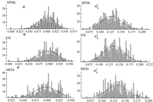
To illustrate the EIS method, our modified EIS method and the SPDK method, we consider a simulation study for a time-varying model for counts with density (6), with time-varying signal θt specified by (2) and (3) and with state initialisation α1 ∼ N(0, σ2η/(1−φ2)). We
simulate time series of counts yt for t= 1, . . . , n and n = 1000. The parameter vector is set
equal to (φ,logσ2
η) = (0.9,−2). For each simulated time series, we estimate the two unknown
parameter coefficients of ψ by maximizing the simulated likelihood function as defined by (13). For the numerical maximisation we adopt the BFGS optimization algorithm with starting values equal to the true parameter values. Likelihood evaluation is based on three methods SPDK, EIS and the modified EIS (MEIS). For the EIS and MEIS methods, we take
M = 50 draws for constructing the importance density. Subsequently, we take M = 500 draws for the Monte Carlo likelihood evaluation. The empirical distributions of the estimates
for the two parameters and for the three methods are presented in Figure 1. Although the empirical distributions are different from each other, for each parameter the distributions are centered around the true parameter values while the variations around the sample mean have similar sizes. However, the computer times for the three different methods are different. SPDK is fast as it fully relies on state space methods. The EIS method is slow since the construction of the importance density also relies on simulation. In the MEIS method, the importance density is obtained using state space methods and is therefore almost as fast as the SPDK method. 0.800 0.825 0.850 0.875 0.900 0.925 0.950 0.975 10 20 30 φ SPDK σ2 η 0.075 0.100 0.125 0.150 0.175 0.200 10 20 30 SPDK 0.800 0.825 0.850 0.875 0.900 0.925 0.950 10 20 30 EIS φ 0.075 0.100 0.125 0.150 0.175 0.200 0.225 10 20 σ2 η EIS 0.825 0.850 0.875 0.900 0.925 0.950 10 20 30 40 φ MEIS 0.075 0.100 0.125 0.150 0.175 0.200 10 20 30 σ2η MEIS
Figure 1: Empirical distributions for the two parameters of the time-varying model for counts as estimated by the three methods SPDK, EIS and the modified EIS (MEIS).
5.2
Stochastic volatility model for pound/dollar exchange rates
To empirically illustrate our modified EIS method, we analyse the volatility of log returns of pound/dollar exchange rates from 1-Oct-1981 to 28-Jun-1985 which is time series also analysed by Harvey, Ruiz, and Shephard (1994) and Durbin and Koopman (2001). The stochastic volatility model is specified as (5) with time-varying signalθt that is specified by
takes place using the modified EIS method. The first step is to find a suitable approximating linear Gaussian state space model to (5) with the observation density given by
ˆ
yt =θt+ut, ut∼N 0, d−t1
, t= 1, . . . , n, (19)
where ˆyt=bt/dt and where the coefficients bt and dt are obtained via applying least squares
computations (16) repeatedly and are evaluated at the simulated samplesθ1, . . . , θM from the
importance density g(θ|yˆ) with ˆy = (ˆy1, . . . ,yˆn)′. Simulation takes place via the simulation
smoother of Durbin and Koopman (2002). The iteration process is initialised with the second-order Taylor coefficients evaluated at the mode. Once the coefficients have converged in the iteration process, we have obtained the importance density and the Monte Carlo estimate of the loglikelihood function can be evaluated.
The BFGS method is used to maximise the simulated loglikelihood function with respect to the parameter vector. The estimates of ˆφ, ˆσ2
η and ˆσ together with its standard errors are
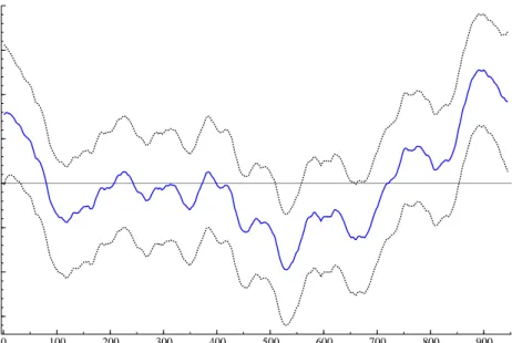
presented for the SPDK and MEIS methods in Table 5.2. We can conclude that the values of the estimated parameters obtained from the SPDK and MEIS methods are very close. The estimated volatility with a 95% confidence interval is displayed in Figure 2.
Parameter SPDK MEIS φ 0.9731 0.9750 (0.501) (0.504) ση 0.1726 0.1643 (0.217) (0.223) σ 0.6338 0.6359 (0.103) (0.108)
Table 1: Simulated maximum likelihood parameter estimates for φ, ση, and σ using SPDK
and MEIS methods based on N = 500 draws to estimate the likelihood function. The standard errors of the estimates are displayed between parantheses below.
References
Carter, C. K. and R. Kohn (1994). On Gibbs sampling for state space models.
Biometrika 81, 541–53.
Danielsson, J. and J. F. Richard (1993). Accelerated Gaussian importance sampler with application to dynamic latent variable models.J. Applied Econometrics 8, S153–S174.
0 100 200 300 400 500 600 700 800 900 −1.5 −1.0 −0.5 0.0 0.5 1.0 1.5 2.0
Figure 2: Estimated volatility process and the 95% confidence interval for the log returns of pound/dollar exchange rates from 1-Oct-1981 to 28-Jun-1985.
de Jong, P. and N. Shephard (1995). The simulation smoother for time series models.
Biometrika 82, 339–50.
Durbin, J. and S. J. Koopman (1997). Monte Carlo maximum likelihood estimation for non-Gaussian state space models.Biometrika 84, 669–84.
Durbin, J. and S. J. Koopman (2001). Time Series Analysis by State Space Methods. Oxford: Oxford University Press.
Durbin, J. and S. J. Koopman (2002). A simple and efficient simulation smoother for state space time series analysis.Biometrika 89, 603–16.
Fruhwirth-Schnatter, S. (1994). Data augmentation and dynamic linear models. J. Time Series Analysis 15, 183–202.
Geweke, J. (1989). Bayesian inference in econometric models using Monte Carlo integra-tion. Econometrica 57, 1317–39.
Harvey, A. C., E. Ruiz, and N. Shephard (1994). Multivariate stochastic variance models.
Rev. Economic Studies 61, 247–64.
Jungbacker, B. and S. J. Koopman (2007). Monte Carlo estimation for nonlinear non-Gaussian state space models. Biometrika 94, 827–39.
an application of integration by monte carlo.Econometrica 46, 1–20.
Liesenfeld, R. and J. F. Richard (2003). Univariate and multivariate stochastic volatility models: Estimation and diagnostics. J. Empirical Finance 10, 505–531.
Richard, J. F. and W. Zhang (2007). Efficient high-dimensional importance sampling. J. Econometrics 141, 1385–1411.
Ripley, B. D. (1987). Stochastic Simulation. New York: Wiley.
Shephard, N. (2005). Stochastic Volatility: Selected Readings. Oxford: Oxford University Press.
Shephard, N. and M. K. Pitt (1997). Likelihood analysis of non-Gaussian measurement time series. Biometrika 84, 653–67.
So, M. K. P. (2003). Posterior mode estimation for nonlinear and non-Gaussian state space models. Statistica Sinica 13, 255–274.