Practice What You Preach: Microfinance Business Models and
Operational Efficiency
IJaap W.B. Bosa,∗, Matteo Millonea
aMaastricht University School of Business and Economics, P.O. Box 616, 6200 MD, Maastricht, The Netherlands
Abstract
We analyze the efficiency of microfinance institutions (MFIs) by modelling their output as a function of number of loans, average loan size and yield on gross portfolio. Our model allows us to take into account the preferences of MFIs as a mix of outreach and financial performance. We estimate a multi-output production possibility frontier with Stochastic Frontier Analysis and find that there is a non-linear negative relationship between number of loans and average loan size. This implies that mission drift will not only reduce depth but also breadth of outreach. Using the estimated efficiency scores, we show that increasing the size of loans and the total size of the loan portfolio actually decreases efficiency. When we take social performance into account, we find that over lending and the percentage of women borrowers have a negative effect on efficiency. We observe no effect on efficiency of multiple borrowing. Increasing the average loan size does not allow MFIs to lend more and does not improve efficiency.
Keywords: microfinance, output distance function, social responsibility, sustainability JEL:G21, O12, O16, C1
1. Introduction
At the center of the current debate about the future of microfinance, is the question whether microfi-nance institutions (MFIs) should be profit-oriented, privately funded, self-sustaining businesses or socially minded, subsidized, not-for-profit organizations (Morduch, 2000). At the heart of the discussion is the often-implicit disagreement regarding how MFIs can operate most efficiently, and with that the disagree-ment regarding what constitutes operational efficiency in microfinance in the first place. Should MFIs be compared based on their profitability or based on their outreach, i.e., the extent to which they provide fi-nancial services to those that were previously deprived of these services? The answer to that question is important, as it helps MFIs direct efforts to improve their performance and informs (institutional) investors regarding MFIs’ (relative) performance.
In this paper, we argue that reality is more contumacious than either side of the above-described de-bate suggests. Just like investors, MFIs have heterogenous preferences: some only care about financial performance, whereas others are mostly oriented towards social performance (i.e., outreach). Others are, quite literally, somewhere in between. Our view of MFIs allows us to develop and estimate a simple model where institutions produce an output that maximizes financial performance (yield), an output that max-imizes scale (average loan size) and an output that maxmax-imizes the breadth of outreach (the number of loans).1 Since our production model also includes MFIs’ inputs (labor, capital), our approach allows us to ask a number of important questions.
IWe are grateful to Luis Orea, participants of the 2012 North American Productivity Workshop in Houston and seminar partici-pants at Maastricht University for helpful comments and discussions. The usual disclaimer applies
∗Corresponding author.
Email addresses:[email protected](Jaap W.B. Bos),[email protected](Matteo Millone)
1In the microfinance literature, the focus on financial revenues is seen as a decrease in the affordability of the loans and increasing
First, we ask whether and to what extent there is a trade-off between each objective (i.e., each output), assuming that all inputs have been used efficiently. At the production frontier, how much depth of outreach has to be sacrificed for a higher yield? Is it possible to combine increases in thedepthof outreach, i.e., small average loan size, with a widerbreadthof outreach? Our paper contributes to the literature by estimating these tradeoffs while controlling for existing slack in MFIs’ production in either direction. Doing so is important, as we may otherwise over- or under-estimate trade-offs: think for example of an MFI that is trying to maximize outreach (depth and width), but does so rather poorly. Not accounting for that poor performance would lead to an overestimation of the trade-off between financial and social performance.
Second, we ask whether the operational efficiency of MFIs depends on their revealed preferences. Are MFIs that are purely profit maximizers more efficient than MFIs that try to maximize outreach? Is there an optimal balance between either objective? Our paper contributes to the literature by estimating the efficiency of MFIs in a setting that accommodates their multi-output nature. Measuring efficiency in this setting is important, as it allows both MFIs and investors to benchmark institutionsgiventheir focus on financial performance, social performance or a mix of both. For example, an institutional investor wishing to invest in microfinance as part of its CSR strategy can invest in the most efficient among the MFIs that focus on outreach.
Third, and related, we ask how MFIs can become more efficient. After all, the investor mentioned in the above example can also choose to invest in an inefficient MFI, opting to boost its efficiency through engagement. How should it do so? Is lending to women indeed a good way to increase outreach (Dowla and Barua, 2006)? What is the nature of the risk-return relationship in microfinance (Mersland and Strøm, 2009)? What is the effect of disbursing multiple loans per client (Krishnaswamy, 2007)? Our paper ad-dresses these issues in a coherent framework, measuring the effects of operational changes and uncovering the different business models that appear to explain the performance of different types of MFIs. Impor-tantly, our analysis can help repudiate the claim that a panacea exists to 'fix' microfinance: what may work for one institution may not work for another institution. However, institutions with a similar output mix may be able to learn from industry best practices.
In order to answer each of these questions, we estimate a multi-output, multi-input production frontier. We use an output distance model (Cuesta and Orea, 2002), control for unobserved institutional differences using a 'true fixed effects' stochastic frontier model (Greene, 2005), and condition efficiency on a number of choice variables following Battese and Coelli (1988). We use the Microfinance Information Exchange (MIX) data, and compare 1,146 MFIs over the period from 2003 to 2010. Our analysis encompasses both strictly for-profit MFIs and firms with a social mission.
Our results show that mission drift does not only decrease depth, but also breadth of outreach, as evi-denced by the negative output elasticity of average loan size with the number of loans. In fact, this negative relationship becomes more pronounced as the average loan size increases. Interestingly, on average, larger loans will result in a lower yield on the gross loan portfolio. Larger loans are also correlated with higher personnel and financing costs. We find support for this finding in the literature, as Mersland (2009) shows that the lower operating costs reported by for-profit MFIs are just an artifice of larger loans. As a matter of fact NGOs have lower costs per loan. According to Gutiérrez-Nieto et al. (2007), NGOs that rely on voluntary work have low personnel costs and thus are able to efficiently offer a large number of small loans.
In addition, we find that, contrary to Hermes et al. (2011), MFIs can indeed combine the depth and breadth of outreach, and operate with above average levels of efficiency. However, efficiency quickly de-creases with the loan portfolio, and high interest rates are not able to offset the inefficiencies caused by mission drift. These findings are in line with the theoretical predictions of Mersland (2009): NGOs and credit cooperative are more efficient as they are able to lower the costs of market contracts. Such institu-tions are not profit maximizers and mainly operate via group loans, this makes them better equipped to cope with highly inefficient markets and asymmetric information. Roberts (2012) shows empirically that a stronger profit orientation leads to higher interest rates, but is also associated with higher costs.
Finally, we find that lending to women, over-lending and increasing the overall riskiness of the loan portfolio all have a negative effect on efficiency. This is consistent with Cull et al. (2007) and Mersland and Strøm (2011) who show that MFIs that focus on lending to women are respectively less profitable and less
efficient.
The remainder of this paper continues as follows. In Section 2, we review the existing literature on microfinance and the performance of MFIs. In Section 3, we introduce our analytical framework, empirical model and estimation strategy. In Section 4, we discuss our data set. Section 5 contains our results. We conclude in Section 6.
2. Literature Review
Once considered the panacea for pulling the un-bankable out of poverty, microfinance has recently come under heavy scrutiny from the public, the media and regulators. The limits of the model developed by Mohammed Yunus are not new to the academic literature. Issues of sustainability, trade-offs between social and financial goals and more recently, efficiency have been the subject of extensive research by both academics and practitioners. The body of research on microfinance is, nevertheless, very heterogeneous in terms of objectives, methodologies and empirical techniques. In this section, we review some of the main findings.
Morduch (1999b), in questioning the self-reported success of Grameer Bank, is one of the first to chal-lenge the notion of microfinance as a sustainable solution to poverty. When taking a closer look at the bank’s financial reports, he finds that the repayment rates are not as good as they claim to be. Furthermore, he finds that, despite reporting profits, Grameer has constantly been subsidized. The findings of Morduch call into question the idea of microfinance as a profitable and yet socially oriented business.
The original view on microfinance was that MFIs following traditional, good banking practices would be the best at alleviating poverty. Morduch (1999a) shows that the 'win-win' proposition is not realistic, both logically and empirically. Given the high costs of lending to the poor, the double bottom line propo-sition can be sustained only if poor borrowers strictly care about access to and not about the cost of credit (Morduch, 2000). Acknowledging that microfinance cannot be profitable and fully socially oriented at the same time is at the origin of what Morduch defines as 'the microfinance schism.'
From that point onwards, the debate on the role and the future of microfinance is dominated by two contrasting views: institutionalist and welfarist (Brau and Woller, 2004). Whereas both views assume that there is a trade-off between financial and social performance, they draw different inferences. The institutionalist view claims that in order to successfully provide financial services to the poor it is necessary to prioritize financial sustainability. The welfarist view focuses on social performance and considers the reliance on donations as necessary and justifiable, given the poverty reduction mission of MFIs.
The trade-off between financial and social performance itself, is mainly attributed to the higher costs of giving out smaller loans. Von Pischke (1996) distinguishes between demand and supply side effects. On the demand side, as the breadth of outreach increases, the probability of lending to risky borrowers increases as well, resulting in an overall riskier portfolio, with more defaults. On the supply side, smaller loans will lead to higher costs, both fixed and variable. This is a consequence of the fact that micro loans are information intensive and have high monitoring costs (Conning, 1999). Fixed costs are not a problem for sustainability as they can be lowered with economies of scale. Variable monitoring costs could be covered by higher interest rates, but this might worsen repayment rates. Poorer borrowers require smaller and more expensive loans that will in turn decrease profitability.
Discussions about the trade-off between financial and social performance gained momentum as a result of mission drift, i.e., the observed tendency of MFIs to move toward richer borrowers by disbursing larger loans. Copestake (2007) frames the decision in the context of a production possibility frontier, where an increase in size leads to economies of scale, allowing the MFI to focus on both depth and breadth of out-reach. Since his model is dynamic, a current decrease in social performance may justify an increase in the size of an MFI in the near future. According to Ghosh and Tassel (2008), mission drift itself is the inevitable response of effective MFIs to the entry of profit-oriented investors in Microfinance. Gonzalez (2010) and Mersland and Strøm (2010) show that larger loans indeed reduce operating expenses and increase profits.
Nevertheless, empirically testing the trade-off between financial and social performance poses a num-ber of challenges. First, it is hard to distinguish between mission drift and cross-subsidization (Armendáriz
and Szafarz, 2010). Second, a decrease in loan size often leads to higher interest rates. According to Mers-land and Strøm (2011), "[T]he balance between outreach to the poor and financial sustainability is to a large extent a question of charging sustainable levels of interest rates since the cost of lending small amount is relatively high" (Mersland and Strøm, 2011, p.3). They show that MFIs do not exercise monopoly power and that the high levels of interest rates are caused by increases in input prices and not by high margins. Cull et al. (2007) find a trade-off between the size and number of loans disbursed, and show that even if smaller loans have higher interest payments, they do not have lower repayment rates.
Meanwhile, the trade-off may depend on institutional characteristics, and can therefore differ from one MFI to the next. Mersland and Strøm (2009) look at the effects of corporate governance on the performance of MFIs. They find that most corporate governance characteristics and ownership structures have very lim-ited or no influence on measures of outreach and financial performance. Cull and Spreng (2011) analyze the case of the privatization of the National Bank of Commerce in Tanzania. They show that even if pri-vatization was difficult, it has led to increases in efficiency while maintaining the same level of outreach. In this particular case outreach and efficiency are not negatively related. Nawaz et al. (2011) show that MFIs with bank status specializing in individual lending tend to be financially efficient, while unregulated NGOs are more socially efficient (Nawaz et al., 2011). Hermes et al. (2011) use a stochastic frontier produc-tion model to see whether depth of outreach is related to inefficiency. They find that smaller loan size leads to a decrease in efficiency.
Summing up, although we have come a long way in improving our understanding of the performance of MFIs, important questions have remained unanswered. In the presence of inefficiency, what is the trade-off between financial and social performance for inefficient MFIs? Is there a trade-trade-off between breadth and depth of outreach? How do lending choices affect operational inefficiency, and thereby the trade-off? In order to answer these questions, we now introduce our approach to model and analyze MFI performance.
3. Methodology
In this section, we introduce our approach to modeling the dual objectives (profit-maximization, out-reach) of MFIs. As the literature review in the previous section has shown, the potential trade-off between these objectives has been analyzed at length. Our approach differs from the literature because we start from the premise that different institutions have different revealed preferences regarding whether to maximize social or financial performance. In our model, an MFI is not penalized for preferring one objective over the other. Rather, an MFI is penalized (i.e., it is inefficient) if - given its use of inputs - it is less successful than other MFIs with the same revealed preferences.
Before we introduce our model in Section 3.2, we first revisit the notion of a trade-off between financial and social performance in microfinance. In Section 3.1, we explain the relationship between that trade-off and our notion of inefficiency.
3.1. Modeling trade-offs and inefficiency
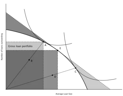
Our objective is to model the trade-off between financial and social performance in a production setting, taking into account the role of operational inefficiency. Therefore, the first question we need to ask is, what constitutes an MFI’s production set. The obvious choice for a measure of output in microfinance is gross loan portfolio (GLP). However, MFIs with the same size gross loan portfolio might be quite different in terms of the number and size of the loans they offer. Suppose an MFI tries to maximize both average loan size (ALS) and the number of loans (NL). In the presence of economies of scale, a higher average loan size will increase profitability, whereas a lower average loan size is traditionally seen as an increase in the depth of outreach. Recent research (Gonzalez, 2010; Mersland and Strøm, 2010; Hermes et al., 2011) shows that loan size is positively correlated with profits and negatively with operating costs. Keeping the level of funding constant, MFIs that focus on social performance (outreach) will disburse a larger amount of smaller loans compared to fewer larger loans offered by financially oriented institutions. A higher number of loans therefore means an increase in the breadth and depth of outreach. In maximizing both average loan size and number of loans, the MFI maximizes the size of its gross loan portfolio.
Figure 1: Theoretical model
Average Loan Size
Number of loans outstanding
C A
B
D Gross loan portfolio
E
Figure 1 is a graphical representation of this trade-off between average loan size and number of loans. In the figure, we assume that an MFI is free to choose its combination of average loan size and number of loans, given its (as yet unspecified) inputs and technology. MFIs are constrained by the amount of funding given a certain level of costs. The constraint is represented graphically by the concave line in Figure 1. Every point on the line represents an efficient combination of average loan size and number of loans, and consequently the area under each point in the curve (such as point A) is equal to gross loan portfolio. Any combination of average loan size and number of loans lying under the frontier line corresponds to an inefficient output mix.
Increasing the number of borrowers will increase outreach (both depth and breadth), but there will also be an increase in operating costs, which in turn will lead to a decrease in the size of gross loan portfolio. This is represented by the darkest shaded area in Figure 1. Increasing average loan size will reduce operating costs, but the gains in costs may be off-set by the increased difficulty in finding borrowers willing to take out bigger loans. As a consequence of mission drift the amount of subsidies received by the MFIs might decrease given their movement away from poor borrowers. The negative impact of increasing average loan size on gross loan portfolio is represented by the lightest shaded area in Figure 1.
We define the utility function of an MFI as:
U(NL,ALS) =NLαALS1−α (1)
An MFI can allocate its portfolio by deciding how many loans to disburse and their size in order to maximize its utility. The two indifference curves in Figure 1 represent all possible combinations of number of loans and average loan size that yield the same level of utility, but given different preferences. An MFI whose indifference curve is tangent to the production possibility frontier in pointC, has a higher preference for average loan size (consequently, it cares less about the breadth of outreach) than an MFI who’s indifference curve is tangent in pointD.
Higher values ofαrepresent a stronger focus of the MFI on outreach, conversely whenαdecreases the
MFIs utility increases relatively more with mission drift. Ifαis equal to 0.5 then the MFI wants to maximize
output. Given a value forαeach MFI maximizes its utility by choosing the ALS and corresponding number
of loans for which the indifference curve is tangent to the financing constraint.
If an MFI is producing at point AorC, we will consider it as efficient even if the GLP is maximized at pointE. If fact both AandCare optimal given the shape of the utility function. Higher costs are the
result of the decision to prioritise the number of loans rather than the loan size, this cannot be considered an inefficiency. PointsBandDrepresent instead inefficient output mixes, because at each of these points one output dimension could be increased without reducing the other.
In the next subsection, we shall extend this view of the trade-offs in microfinance by introducing a more formal modelling approach. In doing so, we introduce the inputs an MFI requires to produce, explain the notion of efficiency in a multi-output setting, and further refine the measurement of an MFI’s outputs in order to distinguish between profitability, depth of outreach and breadth of outreach.
3.2. Output Distance Function
Figure 1 depicts the production possibility frontier, forgiveninput quantities. In order to assess how efficient MFIs transform inputs into outputs, we need to define the possible input-output combinations. Following Cuesta and Orea (2002), forMinputs,Noutputs and a transformation functionTthat satisfies the usual conditions (Färe and Primont, 1995), we define:
T={(x,y):x ∈ <N
+,y∈ <+M,xcan producey}. (2)
So, in fact, for an input vectorx, Figure 1 displays the set of feasible output vectors,y. Denoting the latter asP(x), we can define the distance to the frontier as:2
D0(x,y) =min. n Ψ>0 : y Ψ ∈P(x) o (3) This so-called distance function takes a value of one if an output combination lies on the production fron-tier, otherwise its value is less than one, withD0(x,y)ify ∈ P(x). A key assumption for this function is that outputs can only be reduced if the reduction is proportional, i.e., it may not be possible to reduce one of the outputs while keeping the others constant. Clearly, in the context of our analysis, this is a reasonable assumption.
As shown by Cuesta and Orea (2002) and others,D0(x,y)can be interpreted as an efficiency measure, since it is the inverse of the well-known output-oriented Farrell measure of operational efficiency. Formally, Koopmans (1951) defines a producer as operationally efficient when, in order to increase one output, at least one other output needs to be reduced or a least one input increased.3
The next step, is to derive the vectorMof outputs. For now, let us assume that total outputYis equal to the value added of the MFI’s loan portfolio. LetRybe the average yield on a loan,NLis the number of
loans, andALSis the average loan size. Then we can write total outputYas: Y≡ Ry 1 |{z} Yield (Ry) · NL 1 |{z} Number of loans (NL) · GLP NL | {z } Average loan size (ALS)
(4)
The result isRy·GLP, or the value added of the gross loan portfolio.4
In line with the intermediation approach that has become the standard in the banking literature, we assume that an MFI uses three inputs: financial capital (funds), physical capital (buildings, equipment, etc.) and labor (personnel). These are measured as financial expenses (Xf in), administrative expenses
(Xphys) and personnel expenses (Xlabor), respectively.
2In short, equation (5) is non-decreasing, positively linearly homogeneous and convex in outputs, and decreasing in inputs. 3The measurement of efficiency comes from Debreu (1951) and Farrell (1957) and is defined as "the maximum radial expansion in
all outputs that is feasible with given technology and inputs" (Fried et al., 2008, p.20). Therefore, an efficiency measure of one means that the producer is fully efficient.
4Note that here we can explain why the relationship between average loan size and the number of loans can be characterized by
the down-ward sloping curve in Figure 1. After all, we can rewrite equation (4) asGLPNL =ALS= f(Xf inR,Xyphys·NL,Xlabor). It is straightfor-ward to see that∂ALS
∂NL =−NL12
f(Xf in,Xphys,Xlabor)
We use a translog functional form to represent the technology, and will include a series of regulation dummies (Dlegal) to account for different types of institutions as in Hermes et al. (2011). Letting lnyNitbe
ln(ALSit), we can therefore write the output distance function as: −ln(yit) =αi+ M
∑
k=1 αklnxkit+ N−1∑
j=1 βjlny∗jit+ 1 2 M∑
k=1 M∑
h=1 αkhlnxkitlnxhit +1 2 N−1∑
j=1 N−1∑
h=1 βjhlny∗jitlny∗hit+ M∑
k=1 N−1∑
j=1 αkhlnxkitlny∗hit + M∑
k=1 4∑
legal=1 ζkiDlegallnxkit+ N−1∑
j=1 4∑
legal=1 τjiDlegallny∗jit+uit+vit, (5)wherey∗jit = yjit/yNitto ensure linear homogeneity in outputs, j = 1, 2, and yjit representsYieldit and
NLit, respectively.5,6 The composite error termuit+vit consists of a standard noise term noise term,vit,
and an inefficiency component uit ≥ 0, which is assumed to be i.i.d., with a distribution truncated at µ, |N(µ,σu2)|, and independent from the noise term.7 Efficiency, exp{−uit}, is measured as the ratio of
actual over maximum output, exp{−uit}= YYit∗
it, where 0≤exp{−uit} ≤1, and exp{−uit}=1 implies full efficiency.
Following Färe and Primont (1996), the output distance function should be non-decreasing in outputs and decreasing in inputs. We can verify whether this holds, by evaluating the sum of the estimated input elasticities:8 − M
∑
k=1 δlnD0(yit,xit)/δlnxit. (6)At the means of outputs and inputs, we expect a value significantly greater than one, indicating increasing scale economies. Likewise, to investigate the presence of trade-offs between MFIs’ outputs, we evaluate:
δlnD0(yit,xit)/δlnyjtfori6=j, (7)
where a negative value indicates the existence of a trade-off.
Finally, in order to assess how MFIs can become more efficient, we follow Battese and Coelli (1988), and conditionµ, the truncation point for the inefficiency distribution, as follows:
µit =δ0+δ1ln(PAR30it·Gross Loan Portfolioit) +δ2ln(Number of Women Borrowersit) +δ3ln(Number of Loansit/Number of Borrowersit),
(8) wherePAR30it∗GrossLoanPor f olioit is the amount of portfolio at risk and a measure of portfolio quality,
Numbero f WomenBorrowersit is an alternative measure of depth of outreach and Numbero f Loansit over
Numbero f Borrowersit is a measure of over lending. To control for possible multicollinearity, the variables that explainµhave been orthogonalized.
Summing up, we have now developed an empirical model that allows us to explore the trade-off be-tween financial performance and social performance, to benchmark the efficiency of MFIs, and to assess the factors that can improve that efficiency. In the next section, we introduce our data.
5Ify
ni=yNi, the ratioy∗niis equal to unity. Since the log of this ratio is zero, we effectively sum overN−1 outputs in equation (5).
6To correct for spurious interaction terms, all variables in the translog have been transformed following the Frisch-Waugh
theo-rem.
7In estimating equation (5), we identify the components of the composite error term by re-parameterizingλin a maximum
likelihood procedure, whereλ(=σu/σv) is the ratio of the standard deviation of efficiency over the standard deviation of the noise term, andσ(= (σu2+σv2)1/2) is the composite standard deviation. The frontier can be identified by theλfor which the log likelihood is maximized (see Kumbhakar and Lovell, 2000).
4. Data
We use a publicly available dataset from the Microfinance Information Exchange market (www.mix.org). The MIX dataset collects self-reported balance sheet information and is widely used in the literature (Cull et al., 2009; Ahlin et al., 2011; Hermes et al., 2011; Roberts, 2012). In total, MIX includes 1,146 MFIs, over the period 2003-2010. After eliminating outliers, we have an unbalanced panel with 3,890 observations.9 Table 1 reports mean values, sorted by the legal status of the institution.10
Table 1: Descriptive statistics by legal statusa
Bank Cooperative NBFI NGO Other Rural Bank Total
Outputs
Average Loan Sizeb 1627.5 2017.2 1143.6 625.7 1115.0 571.0 1048.9
(1779.6) (2108.5) (2095.7) (1143.4) (2148.9) (558.6) (1752.9)
Number of Loans 78131.9 13836.9 49354.5 42053.1 18287 20599.7 42070.4
(118295.0) (24557.2) (110585.5) (80089.3) (27780.8) (32961.5) (89640.2)
Yield on gross loan portfolio (ygp_r)c 0.24 0.16 0.26 0.27 0.24 0.21 0.25
(0.16) (0.09) (0.15) (0.15) (0.17) (0.10) (0.15)
Inputs
Financial expenses (FiExp/Ass)d 0.056 0.057 0.056 0.047 0.067 0.050 0.052
(0.032) (0.053) (0.033) (0.031) (0.039) (0.026) (0.036)
Personnel expenses (PExp/Ass)d 0.086 0.055 0.10 0.11 0.092 0.065 0.098
(0.046) (0.034) (0.066) (0.069) (0.070) (0.031) (0.065)
Administrative expenses (AdExp/Ass)d 0.079 0.057 0.083 0.083 0.076 0.061 0.078
(0.056) (0.038) (0.053) (0.059) (0.059) (0.034) (0.055)
Determinants Portfolio at risk 30e 0.054 0.064 0.051 0.057 0.037 0.096 0.057
(0.081) (0.068) (0.064) (0.076) (0.048) (0.088) (0.073) % women borrowers 53.0 50.6 61.8 74.5 70.7 53.9 64.7 (21.9) (21.5) (25.1) (23.6) (27.1) (28.4) (25.6) Over-lendingf 1.06 1.06 1.05 1.05 1.14 1.06 1.05 (0.11) (0.21) (0.18) (0.23) (0.38) (0.14) (0.21) Costs
Costs per borrower 298.4 231.5 232.7 126.6 306.3 110.2 186.7
(280.8) (179.6) (570.9) (232.8) (428.9) (85.1) (382.7)
Costs per loan 283.9 219.2 221.1 115.2 220.9 106.4 175.0
(275.8) (170.5) (556.9) (128.5) (278.1) (84.5) (352.2)
Total expenses 23.7 17.4 25.8 26.3 21.4 18.6 24.5
(9.83) (8.05) (12.0) (12.7) (13.4) (6.76) (12.0)
aNumber of observations is 3,890; standard deviation in parentheses; all monetary values in USD, corrected for inflation. Cooperative
is a cooperative or a credit union; NBFI is a non-bank financial institution; NGO is a non-governmental organisation.
bAverage loan size in USD. cYield on gross loan portfolio: one percent is 0.01.
dInputs are scaled by assets for comparative purposes, but included non-scaled in the estimations of the output distance frontier. ePortfolio at risk, 30 days late for payment. fOver-lending defined as number of loans over number of borrowers.
The first thing to observe from Table 1, is the large heterogeneity among MFIs. On the one end of the spectrum, we find banks, who are the largest institutions in the sample, offer large loans and seem to be indifferent between lending to men or women. Despite the fact that banks on average give out large loans, they have relatively high costs per borrower, suggesting that they are not able to benefit from economies of scale. Nevertheless, and consistent with their profit motive, banks have a high yield on gross loan portfolio (although it is not the highest).
On the other end of the spectrum we have rural banks, who despite their small size and small loans have low costs per borrower and a lower yield. Credit unions are the best performers in terms of affordability and profitability, but offer some of the largest loans. Both credit unions and non-bank financial institutions
9We excluded the top and bottom percentiles.
(NBFI) are small in size, but NBFIs offer smaller loans, which in turn leads to higher yield on gross portfolio. NGOs are the smallest institutions, offer the smallest loans and almost three quarters of their borrowers are women. The cost per borrower reported by NGOs is one of the lowest, but at the same time the yield on gross portfolio is the highest in the sample.
Summing up, based on the descriptive statistics in Table 1, we can observe that it is not obvious that there are economies of scale, since larger institutions do not report lower average costs. Also, for-profit in-stitutions do not report lower total expenses or average costs, invalidating claims of superior management quality. In addition, institutions that offer larger loans tend to charge lower interest rates. Finally, high yields on gross portfolio seem to be unrelated to costs per borrower, but might instead be a consequence of the higher credit risk of smaller loans.
Nevertheless, these results need to be interpreted carefully for two reasons. First, low costs per borrow-ers reported by NGOs and Rural Banks will be influenced by subsidies, for which we have no data. Second, a significant number of institutions may be operating inside the production possibility frontier and might still be able to improve their performance in multiple dimensions.
The evidence reported in Table 1 supports the empirical specification of our model. It shows that there are indeed strong differences in the gross loan portfolio composition, costs and yield among MFIs. This justifies the use of a production function with multiple outputs. Additionally, the heterogeneity across legal statuses gives reasons for using institution type dummies in the specification of the output distance function.
5. Results
In this section, we discuss our empirical results. First, we investigate whether there is indeed a trade-off between financial and social performance. Second, we investigate whether operational efficiency of MFIs depends on their revealed preferences, i.e., their output mix. Third, we investigate how MFIs can improve their operational efficiency.
5.1. Is there a trade-off between financial and social performance?
We start by empirically assessing the existence of a trade-off between financial performance and social performance, i.e., the non-existence of the so-called double bottom line. We do so by evaluating the output cross-elasticities, both at the mean and across the sample ranges. Since the average loan size is our left-hand side variable, a trade-off implies a positive elasticity with respect to the number of loans as well as with respect to the yield on gross loan portfolio.11 Mean elasticities are reported in Table 2.12 Input elasticities are positive, as expected. Interestingly, on average, we find evidence of decreasing returns to scale, reflected by the fact that the sum of the input elasticities is slightly but significantly smaller than one. Even more interesting are the output trade-offs. First, depth and breadth of outreach are, on average, complements, reflected by a negative elasticity of -0.68 with respect to the number of loans. This means that a higher number of loans on average is accompanied by a lower average loan size. When compared to the simple correlation, which is -0.15, the complementarity is rather strong. Second, financial and social performance are, on average, complements, reflected by a negative elasticity of -0.18 with respect to the yield on gross loan portfolio. This means that a higher yield on gross loan portfolio, ceteris paribus, is accompanied by a lower average loan size. Although the latter elasticity is much smaller than the former, it is significantly different from zero. Therefore, in order to further investigate, we turn to a graphical analysis of the output substitution elasticities, in Figures 2a and 2b.
11Recall that a higher average loan size meanslessdepth of outreach.
12The elasticities are equal to the average fitted value of the first derivative of equation 5 with respect to the variable of interest,
thus controlling for the substitution of inputs and the non-separability of outputs. We test the statistical significance of the estimates using a t-test on the fitted values after taking the first derivative.
Table 2: Output trade-offs and scale economies
Mean Elasticity p-value
Output trade-offs
Elasticity to number of loans -0.68 0.000
Elasticity to yield on gross loan portfolio -0.18 0.000
Scale economies
Elasticity to financial expenses 0.33 0.000
Elasticity to administrative expenses 0.05 0.000
Elasticity to personel expenses 0.56 0.000
Total input elasticity 0.94 0.000
Number of observations is 3,890
Figure 2: Output substitution elasticities (a) Substitution elasticity of average loan size and number of
loans −1 −.8 −.6 −.4 −.2
Elasticity of ALS to number of loans
0 5000 10000 15000 20000
Average Loan Size
(b) Substitution elasticity of average loan size and yield on gross loan portfolio −.6 −.4 −.2 0 .2
Elasticity of ALS to yield on gross portfolio
0 5000 10000 15000 20000
Average Loan Size
In Figure 2a we plot the elasticity of average loan size to the number of loans, i.e., the complementarity between depth and breadth of outreach, as a function of the average loan size. Recall that since alower average loan size increases the depth of outreach, we expect to see a negative relationship if depth and breadth of outreach are complements. Indeed, this is what is shown in Figure 2a across the whole range of average loan size, suggesting that increasing the number of loans offered does not have to result in mission drift. Contrary to Schreiner (2002) we argue that poor breadth of outreach does not need to compensate for profound depth. MFIs do not shift to richer clients in order to finance a larger amount of smaller loans. Therefore our results do not support the idea that increases in average loan size are the result of cross -subsidization (Armendáriz and Szafarz, 2010).
Figure 2b shows the elasticity of average loan size to the yield on gross portfolio, as a function of average loan size. While the average elasticity is -0.18, it is not negative for the whole sample. For the majority of MFIs, decreases in average loan size are accompanied by an increase in the yield on gross portfolio, suggesting MFIs that are maximizing the depth of outreach are also able to maximize revenues, which might be at odds with the microfinance 'mission.' Our finding is consistent with Conning (1999), who reports that institutions that target the poorest are able to do so only by charging higher interest rates. However, for a number of institutions on the right tail of the distribution the relationship is either null or weakly positive. For a subgroup of MFIs it seems possible to offer smallandaffordable loans.
Summing up, charging higher interest rates allows MFIs to reach at the same time higher breadth and depth of outreach. In the next section we are going to show whether such output mix is efficiently achiev-able.
5.2. Does the efficiency of MFIs depend on their output mix?
In this section we are going to investigate the relationship between revealed preferences of the MFIs and operational efficiency. Each MFI’s output mix is a manifestation of its preferences with respect to various measures of performance. Nevertheless maximizing certain dimensions of output might be more challenging than others. For instance an institution targeting richer borrowers in an urban setting might face stiffer competition than a rural lender, who on the other hand will incur in higher travelling costs. In our model, efficiency does not depend only on slack, but also on the choice of output mix. We can finally answer the question of whether MFIs that stick to poorer clients are able to increase breadth of outreach while operating efficiently and whether efficiency is achieved at the cost of affordability of the loans. To find these answers we start by looking at each single output separately and then move to pairwise combinations of outputs.
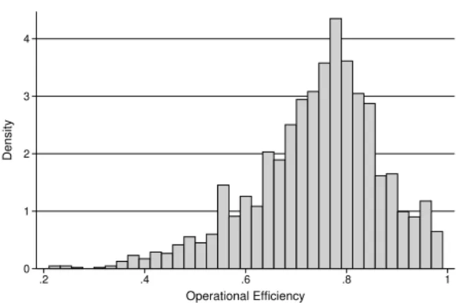
Figure 3: Distribution of efficiency
0 1 2 3 4 Density .2 .4 .6 .8 1 Operational Efficiency
Note: mean efficiency=0.74; standard deviation = 0.13
In Figure 3 we plot the unconditional distribution of efficiency scores. The efficiency scores represent the amount of possible total output produced by an MFI given inputs and technology. An MFI with a score of 90% could increase its total production by 10% given its inputs. As expected the efficiency scores are skewed to the left and do not appear to be multi modals. Efficiency ranges from a minimum of 21% to a maximum of 99% with an average value of 74%. The majority of MFI operates at least at 76% efficiency.
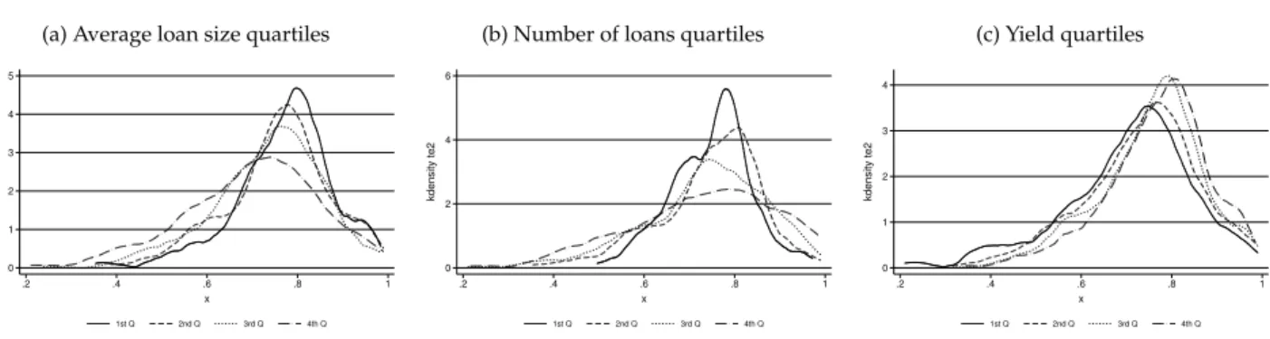
We now focus on the correlation of a particular dimension of output with efficiency. To take into account country effects, we normalized the distribution of ALS and yield on gross portfolio for each country. In Figures 4a, 4b and 4c we plot the kernel distributions of efficiency corresponding to each quartile of our three measures of output. In Table 7, we test the statistical significance of the differences in operational efficiency between subsamples of the distributions. In addition to the common t-test, we use a Kruskal-Wallis (KW) rank test of the equality of population and a Kolmogorov-Smirnov (KS) test of the likeness of the distributions.
In Figure 4a, we show that the distribution of operational efficiency has a stronger left skew and lower variance for lower quartiles of average loan size . The implication is that a higher proportion of MFIs offering small loans is efficient compared to MFIs offering large loans. Hypothesis H01tests whether the distribution of efficiency for the top 50% MFIs in terms of average loan size is significantly different from the bottom 50%. The t test shows that the mean efficiency score for the top 50% is significantly lower that for the to bottom, and the KW and KS respectively confirm that the population and the distribution are significantly different. The hypothesesH20 test the differences among subsequent quartiles and between first and last quartiles, all the tests strongly reject all theH02hypotheses.
These results confirm both the theoretical prediction and the empirical findings of Mersland and Strøm (2010), whom by adapting the model of Freixas and Rochet (1997) to microfinance, show that inefficient
Figure 4: Distribution of efficiency for different output quartiles (a) Average loan size quartiles
0 1 2 3 4 5 kdensity te2 .2 .4 .6 .8 1 x 1st Q 2nd Q 3rd Q 4th Q
(b) Number of loans quartiles
0 2 4 6 kdensity te2 .2 .4 .6 .8 1 x 1st Q 2nd Q 3rd Q 4th Q (c) Yield quartiles 0 1 2 3 4 kdensity te2 .2 .4 .6 .8 1 x 1st Q 2nd Q 3rd Q 4th Q
Explain what this means: allocative, technical and economic efficiency....
MFIs need to shift their portfolio towards larger loans. Interestingly the relationship between efficiency and average loan size is the opposite of what Hermes et al. (2011) find by estimating the model with a single output production function.
Table 3: Hypothesis tests for different output quartiles
Quartiles for: Average loan size Number of loans Yield
Hypothesis t-test KW KS t-test KW KS t-test KW KS
H01:te>average˜ −te≤average˜ =0 0.0000 0.0001 0.0000 H02:teQ1−teQ2=0 0.0052 0.0024 0.0000 0.5480 0.1417 0.0000 0.0000 0.0001 0.0000 H03:teQ2−teQ3=0 0.0000 0.0001 0.0000 0.1157 0.2732 0.0030 0.0002 0.0003 0.0000 H04:teQ3−teQ4=0 0.0000 0.0001 0.0000 0.3689 0.7087 0.0010 0.0065 0.0039 0.0020 H5 0:teQ1−teQ4=0 0.0000 0.0001 0.0000 0.0023 0.3524 0.0000 0.0000 0.0001 0.0000
Notes: KW= Kruskal-Wallis rank test; KS = Kolmogorov-Smirnov test.
Contrary to average loan size, the effect of number of loans on efficiency is not as straight forward to interpret. In Figure 4b the kernel densities show that the distributions are more or less centred around the same point, while the variance increases with number of loans. It is hard to identify a monotonic effect on efficiency, but we can observe higher heterogeneity of efficiency for institutions with higher breadth of outreach. The results of the tests confirm the ambiguity of the effect. Generally, efficiency seems to slightly decrease with the number of loans, but this effect is not statistically significant. Economies of scale resulting from disbursing more loans seem to be offset by the costs of finding suitable borrowers.
Finally, we analyze the effect of yield on gross portfolio on efficiency. In Figure 4c we show that the distribution of efficiency skews to the left for higher quartiles of yield on gross portfolio. In this case we do not observe big differences in the variance. In Table 7 all the tests rejectH50, confirming that the difference in terms of efficiency of the top and bottom half of MFIs ranked by yield on gross portfolio is significant. Testing the differences between quartiles we see that all quartiles are significantly different from the others. We conclude that efficiency monotonically increases with yield on gross portfolio. This result seems to contradict Roberts (2012), but in our context it simply means that charging higher interest rates is an efficiency way to generate revenues given the cost of inputs.
In order to achieve a clearer picture, it is necessary to analyze the interaction between more than one output. In Tables 4a and 4b we tabulate quartiles of average loan size against number of loans, and yield on gross portfolio, respectively. The average efficiency score and number of observation are reported for 16 combinations of quartiles per pair of outputs. We use this tabulation to analyze how differences in output mixes influence the efficiency of the MFIs. We first look at different combinations of depth and breadth of
Table 4: Trade-offs between financial and social performance (a) Average loan size and number of loans
Quartiles ALS 1st 2nd 3rd 4th Total Quartiles NL 1st 0.770 0.763 0.743 0.727 0.748 (210) (237) (207) (318) (972) 2nd 0.774 0.748 0.736 0.712 0.745 (296) (271) (175) (230) (972) 3rd 0.765 0.753 0.732 0.680 0.737 (260) (288) (233) (191) (972) 4th 0.775 0.769 0.729 0.664 0.730 (206) (176) (357) (233) (972) Total 0.771 0.757 0.734 0.699 0.740 (972) (972) (972) (972) (3888)
(b) Average loan size and yield
Quartiles ALS 1st 2nd 3rd 4th Total Quartiles YGP 1st 0.757 0.730 0.703 0.685 0.707 (128) (152) (262) (429) (971) 2nd 0.761 0.754 0.730 0.704 0.733 (167) (230) (282) (293) (972) 3rd 0.776 0.756 0.750 0.725 0.753 (217) (327) (261) (167) (972) 4th 0.777 0.776 0.764 0.702 0.768 (458) (263) (167) (83) (971) Total 0.771 0.757 0.734 0.699 0.740 (970) (972) (972) (972) (3886) Can we test?
outreach and then at depth of outreach and affordability.
In Table 4a we tabulate efficiency scores and number of observations (in parentheses) for quartiles of av-erage loan size against quartiles of number of loans. From the number of observations for each combination we see that the two most common output mixes are either a small number of large loans (row 1, column 4) or a large number of medium loans (row 4, column 3). Nevertheless the frequency of observations is quite evenly distributed, indicating strong heterogeneity in gross loan portfolio composition. Combining this finding with Table 1 it is clear that, when discussing mission drift, MFIs should not be divided in two groups, as they are found in a variety of hybrid forms.
The bottom row in Figure 4b shows that efficiency is significantly lower for MFIs offering the largest loans. When average loans size is below median (first two columns), efficiency scores are always above the sample mean of 74%. Disbursing more or less loans has no effect on the efficiency of MFIs with deep outreach. In the third and fourth columns we show that pretty much all MFIs with shallower depth of outreach operate at below average efficiency. MFIs that offer a small number of large loans score below 74%. With a group average of 64%, the most inefficient MFIs are the ones offering a large number of large loans. As shown by the rapid decrease in efficiency in column 4, inefficiencies related to mission drift become more serious as MFIs switch to larger loans .
We can confidently state that MFIs can achieve both depth and breadth of outreach while operating at high levels of efficiency. If increasing loan size is the response to competition with profit oriented institu-tions (Ghosh and Tassel, 2008), it is the wrong one. MFIs offering many large loans should be experiencing economies of scale (Copestake, 2007), but we find no evidence of loan size improving efficiency. As a mat-ter of fact MFIs that gravitate towards a more traditional approach to banking (high breadth and low depth of outreach) are highly inefficient.
We look at the distribution of efficiency for combinations of loan size and yield on gross portfolio in Table 4b. We confirm the negative relationship between loan size and interest rates, as the most common groups are MFIs that offer large cheap loans (row 1, column 4) and MFIs that charge high interest rates on small loans (row 4, column 1). There are only 83 observations for combinations of high yields and large loans. In line with Morduch (2000), this evidence shows that poorer borrowers have very low price elasticity of demand to loans. The last column of Table 4b shows that yield on gross portfolio has a positive effect on efficiency. The positive effect of yields is consistently strong for the first three quartiles of ALS, but disappears for the biggest loans. MFIs offering large loans do not benefit in terms of efficiency from raising rates. This is probably because of increased competition with the formal banking sector, MFIs are not able to maintain efficiency while offering expensive large loans. Competition makes it more difficult to find good borrowers, increasing both search costs and risk of the portfolio.
that depth of outreach can be achieved efficiently, but at the cost of affordability. Interestingly the top left area of 4b shows that a large number of MFIs are able to offer small cheap loans and still operate at higher than average levels of efficiency.
Across the board, MFIs with larger loans are less efficient. This is at first counterintuitive and contrary to the findings of Hermes et al. (2011), but there are a number of reasons why it is plausible. Firstly, by moving towards a different client base the experience acquired by loan officers and management will be-come less useful as well as some of the lending techniques. Secondly, competition with the formal banking sector will increase forcing the MFIs to either cut rates or accept riskier borrowers. Finally, abandoning the poorest borrowers will decrease the benefits that come with the microfinance status, such as lax regulatory oversight and cheap funding.
Summing up, by analyzing the distribution of efficiency scores we show that mission drift leads to inefficiencies and especially so when MFIs try to offer a large number of large loans or charge high interest rates on them. MFIs that stick to poorer clients are more efficient. This is independent from breadth of outreach or the affordability of the loans offered.
5.3. How can MFIs improve their efficiency?
In this section, we investigate how MFIs could increase their performance without having to modify their preferences. In equation 8 we conditioned the truncation of the distribution of efficiency scores on three exogenous variables. These variables proxy for preferences of the MFIs that are not directly related to the production function, thus cannot be considered as inputs or outputs per se. Our selection of exogenous determinants of efficiency consists of the number of defaults, the percentage of women borrowers and the number of outstanding loans per borrower. These variables are under the direct control of the MFIs management and are therefore an easy tool for investors’ engagement.
Table 5: Operational determinants of efficiency
variables Coefficient Standard Error
Constant 4.279 3.655
ln(PAR30·GrossLoanPort f olio) -0.004 0.039
ln(%Women·Borrowers) -0.278*** 0.057
ln(Loans/Borrowers) -1.209*** 0.537
The amount of portfolio in default measures portfolio quality and risk attitude of the MFIs. Lenders can increase their portfolio quality by requiring collateral and engaging in more screening and monitor-ing. Nevertheless, MFIs usually operate in the absence of collateral, in markets where severe information asymmetry makes screening and monitoring very costly. According to Von Pischke (1996), the probability of lending to risky borrowers increases with breadth of outreach. The coefficient in Table 5 is slightly neg-ative but insignificant. The lack of any effect might be due to the fact that the costs of additional screening and monitoring will offset the benefits of marginally better repayment rates. Thus, efficiency is not affected by portfolio quality.
The percentage of women borrowers is an alternative measure of depth of outreach of the MFI (Schreiner, 2002; Hermes et al., 2011). From the summary statistics in Table 1 we can observe how NGOs and Rural Banks have comparable level of depth of outreach, but are strongly different when it comes to the percent-age of women borrowers. This is an indication of how relevant the original social mission of microfinance is for the institution. The coefficient is negative and significant, which implies that a higher percentage of women borrowers will have a negative effect on the mean of the efficiency distribution. Unfortunately, we can only interpret the sign and significance of the coefficient as it is not a marginal effect. This finding is consistent with Hermes et al. (2011). Despite the fact that women are better borrowers (D’Espallier et al., 2011), Roberts (2012) shows that the emphasis on women borrowers is positively correlated to operating costs and negatively to financial sustainability.
We introduce the ratio of number of loans to number of borrowers as a rough measure of the over-lending of the MFI. Even if over-indebtedness in microfinance is a hotly debated topic (Schicks, 2010), it is a concept hard to define, let alone measure (Alam, 2012). We simply try to identify institutions that are willing to disburse multiple loans for each borrower. We find negative and significant effect of the number of loans per borrower on the truncation of the efficiency score distribution. Laxity in lending strongly reduces efficiency, MFIs should be highly discouraged from allowing borrowers to enter multiple debt contracts.
6. Conclusion
The idea behind microfinance is quite simple: to provide financial services to the poor. In reality, its application is everything but simple. As a consequence of different sets of beliefs, market conditions and business practices, MFIs strongly differ among each other in multiple aspects. This paper aims at bench-marking the efficiency of MFIs but avoids making any restrictions as to what the most relevant performance indicator is. Simply put, we develop and apply a methodology that uncovers which type of MFI will make the most out of its limited resources.
Our main methodological contribution consists in decomposing the value added of gross loan portfolio into three factors: yield on gross portfolio, average loan size and number of loans. Each of these factors proxies for, respectively, financial performance, profitability and outreach. Borrowing from the efficiency literature on banking, we utilize a stochastic frontier true fixed effect model to estimate a multi output cost function and an efficiency score for 1146 MFIs.
From the estimation of the output frontier, we are able to extract the elasticities of average loan size to the other outputs and inputs. We observe that average loan size has, on average, negative elasticity to number of loans. The strength of the negative relationship increases with the size of the loan. MFIs can reach both depth and breadth of outreach, as they move towards better off clients, they need to increasingly diminish the number of loans offered. Our evidence shows that mission drift does not only decrease depth, but also breadth of outreach.
Small loans are not necessarily cheap, as the negative elasticity to yield on gross portfolio shows. On average, larger loans will result in lower yield on gross portfolio. We show that for a limited number of MFIs the elasticity of average loan size to yield is zero or positive. This means that a subgroup of MFIs is able to offer small but cheap loans. Larger loans are also correlated with higher personnel and financial costs.
The relationship between efficiency scores and outputs shows a clearly negative effect of mission drift on performance. MFIs can combine depth and breadth of outreach and maintain above average levels of efficiency. However, efficiency quickly decreases with the size of loans and of the portfolio. Yield on gross portfolio is positively related with efficiency but high interest rates are not able to offset the inefficiencies of mission drift. Nevertheless, we observe again a sizeable group of MFIs that efficiently offer small, and most importantly, affordable loans.
Finally we control for exogenous preferences of the MFIs such as social outreach, risk aversion and over-lending. We see that lending to women has a negative effect on efficiency. This means that a strong focus on the women empowerment goal has to be achieved at the cost of efficiency. MFIs cannot improve their performance by indiscriminately lending more, in fact we show that over lending reduces efficiency.
We interpret our findings as an indication that, in terms of efficiency, transforming MFIs into bank-like for-profit institutions might not pay off. The institutions in our sample are the most efficient when doing what they do best: offering relatively expensive loans to the poor. Moving towards better off clients in an attempt to reap the benefits of economies of scale, lower risk and profit oriented investments leads to an inefficient use of resources. Whether this is the effect of subsidies, lack of managerial skills or changing market conditions, we do not know. What we offer is a simple engagement framework that would be useful for investors and policy makers looking at increasing the effectiveness of microfinance.
References
Ahlin, C., Lin, J., Maio, M., 2011. Where does microfinance flourish? microfinance institution performance in macroeconomic context. Journal of Development Economics 95 (2), 105 – 120.
URLhttp://www.sciencedirect.com/science/article/pii/S0304387810000416
Alam, S. M., 2012. Does microcreidt creat over-indebtedness? Working paper.
Armendáriz, B., Szafarz, A., 2010. On mission drift in microfinance institutions. The Handbook of Microfinance 32 (May 2009), 0–29. Battese, G. E., Coelli, T. J., July 1988. Prediction of firm-level technical efficiencies with a generalized frontier production function and
panel data. Journal of Econometrics 38 (3), 387–399.
Brau, J. C., Woller, G. M., 2004. Microfinance: A comprehensive review of the existing literature. Journal of Entrepreneurial Finance and Business Ventures 9 (1), 1–26.
Conning, J., 1999. Outreach, sustainability and leverage in monitored and peer-monitored lending. Journal of Development Economics 60 (1), 51 – 77.
Copestake, J., 2007. Mainstreaming microfinance: Social performance management or mission drift? World Development 35 (10), 1721 – 1738.
Cuesta, R. A., Orea, L., 2002. Mergers and technical efficiency in spanish savings banks: A stochastic distance function approach. Journal of Banking & Finance 26 (12), 2231–2247.
Cull, R., Demirgüç-Kunt, A., Morduch, J., 2009. Microfinance meets the market. The Journal of Economic Perspectives 23 (1), pp. 167–192.
URLhttp://www.jstor.org/stable/27648299
Cull, R., Demirgüç-Kunt, A., Murduch, J., 2007. Financial performance and outreach: A global analysis of leading microbanks. The Economic Journal 117, F107–F133.
Cull, R., Spreng, C. P., 2011. Pursuing efficiency while maintaining outreach: Bank privatization in tanzania. Journal of Development Economics 94 (2), 254 – 261.
Debreu, G., 1951. The coefficient of resource utilization. Econometrica 19 (3), pp. 273–292.
D’Espallier, B., Gu?l’rin, I., Mersland, R., 2011. Women and repayment in microfinance: A global analysis. World Development 39 (5), 758 – 772.
URLhttp://www.sciencedirect.com/science/article/pii/S0305750X10002330
Dowla, A., Barua, D., 2006. The Poor Always Pay Back: The Grameen II Story. Kumarian Press.
Färe, R., Primont, D., 1995. Multi-output Production and Duality: Theory and Applications. Kluwer Academic Publishers, Boston. Färe, R., Primont, D., 1996. The opportunity cost of duality. Journal of Productivity Analysis 7, 213–224.
Farrell, M. J., 1957. The measurement of productive efficiency. Journal of the Royal Statistical Society 120, 253–281. Freixas, X., Rochet, J., 1997. Microeconomics of Banking. MIT Press, Cambridge.
Fried, H., Lovell, K., Schmidt, S., 2008. The Measurement of Productive Efficiency and Productivity. Oxford University Press. Ghosh, S., Tassel, E. V., Dec. 2008. A model of mission drift in microfinance institutions. Working Papers 08003, Department of
Economics, College of Business, Florida Atlantic University.
Gonzalez, A., August 2010. Microfinance synergies and trade-offs: Social versus financial performance outcomes in 2008. MIX Data Brief 7.
Greene, W., 2005. Fixed and random effects in stochastic frontier models. Journal of Productivity Analysis 23, 7–32, 10.1007/s11123-004-8545-1.
Gutiérrez-Nieto, B., Serrano-Cinca, C., Molinero, C. M., 2007. Microfinance institutions and efficiency. Omega 35 (2), 131 – 142. Hermes, N., Lensink, R., Meesters, A., 2011. Outreach and efficiency of microfinance institutions. World Development 39 (6), 938 –
948.
Kodde, D. A., Palm, F. C., 1986. Wald criteria for jointly testing equality and inequality restrictions. Econometrica 54, 1243–1248. Koopmans, T. C., 1951. An analysis of production as an efficient combination of activities. In: Activity Analysis of Prodcution and
Allocation. Cowels Comminssion for Research in Economics Monograph No. 13. New York: John Wiley & Sons, Ltd.
Krishnaswamy, K., 2007. Competition and multiple borrowing in the indian microfinance sector. Financial Management (September). Kumbhakar, S. C., Lovell, C. A. K., 2000. Stochastic frontier analysis. Cambridge University Press.
Mersland, R., 2009. The cost of ownership in microfinance organizations. World Development 37 (2), 469 – 478. URLhttp://www.sciencedirect.com/science/article/pii/S0305750X08001484
Mersland, R., Strøm, R. Ø., 2009. Performance and governance in microfinance institutions. Journal of Banking & Finance 33 (4), 662 – 669.
Mersland, R., Strøm, R. Ø., 2010. Microfinance mission drift? World Development 38 (1), 28 – 36. Mersland, R., Strøm, R. Ø., 2011. What drives the microfinance lending rate? Working Paper. Morduch, J., 1999a. The microfinance promise. Journal of Economic Literature 37 (4), pp. 1569–1614.
Morduch, J., 1999b. The role of subsidies in microfinance: evidence from the grameen bank. Journal of Development Economics 60 (1), 229 – 248.
Morduch, J., 2000. The microfinance schism. World Development 28 (4), 617 – 629.
Nawaz, A., Hudon, M., Basharat, B., 2011. Does efficiency lead to lower interest rates? a new perspective from microfinance. In: Second European Research Conference in Microfinance, Groningen, The Netherlands.
Roberts, P. W., 2012. The profit orientation of microfinance institutions and effective interest rates. World Development (0), –. URLhttp://www.sciencedirect.com/science/article/pii/S0305750X12001441
Schicks, J., 2010. Microfinance over-indebtedness: Understanding its drivers and challenging the common myths. Working Papers CEB 10-048, ULB – Universite Libre de Bruxelles.
Schreiner, M., 2002. Aspects of outreach: a framework for discussion of the social benefits of microfinance. Journal of International Development 14 (5), 591–603.
URLhttp://dx.doi.org/10.1002/jid.908
Von Pischke, J. D., 1996. Measuring the trade-off between outreach and sustainability of microenterprise lenders. Journal of Interna-tional Development 8 (2), 225–239.
Table 6: Output distance frontier resultsa
Variable Parameter Std.Error
Deterministic Component of Stochastic Frontier Modelb
constant 2.85335*** (0.03966) ln(number of loans) -1.08258*** (0.01589) ln(yield) 0.03966*** (0.00751) ln(financial expenses) -0.03093*** (0.00402) ln(adminstrative expenses) 0.00622 (0.02306) ln(personnel expenses) -0.20798*** (0.02651) 1 2ln(number of loans)2 0.04712*** (0.00448) 1 2ln(yield)2 -0.02195*** (0.00173) 1 2ln(financial expenses)2 0.05451*** (0.00142) 1 2ln(adminstrative expenses)2 0.00491 (0.00613) 1 2ln(personnel expenses)2 0.09317*** (0.00668)
ln(number of loans)×ln(yield) 0.00164*** (0.00008) ln(number of loans)×ln(financial expenses) 0.00036*** (0.00009) ln(number of loans)×ln(adminstrative expenses) 0.00055* (0.00030) ln(number of loans)×ln(personnel expenses) -0.00051 (0.00035) ln(yield)×ln(financial expenses) -0.00029*** (0.00006) ln(yield)×ln(adminstrative expenses) 0.00033** (0.00016) ln(yield)×ln(personnel expenses) 0.00019 (0.00016) ln(financial expenses)×ln(adminstrative expenses) -0.00002 (0.00017) ln(financial expenses)×ln(personnel expenses) -0.00025 (0.00017) ln(adminstrative expenses)×ln(personnel expenses) -0.00055 (0.00040) ln(number of loans)×DBank 0.00614* (0.00327)
ln(number of loans)×DCooperative or credit union 0.00336 (0.00308)
ln(number of loans)×DNon-bank financial institution 0.01025*** (0.00304)
ln(number of loans)×DRural bank 0.00794 (0.01092)
ln(yield)×DBank -0.00201 (0.00206)
ln(yield)×DCooperative or credit union 0.00380** (0.00183)
ln(yield)×DNon-bank financial institution -0.00226 (0.00177)
ln(yield)×DRural bank -0.00669 (0.00548)
ln(financial expenses)×DBank 0.00250 (0.00226)
ln(financial expenses)×DCooperative or credit union -0.02378*** (0.00188)
ln(financial expenses)×DNon-bank financial institution -0.00820*** (0.00138)
ln(financial expenses)×DRural bank 0.00570 (0.00377)
ln(adminstrative expenses)×DBank 0.00938 (0.00630)
ln(adminstrative expenses)×DCooperative or credit union 0.00915** (0.00391)
ln(adminstrative expenses)×DNon-bank financial institution 0.01088* (0.00556)
ln(adminstrative expenses)×DRural bank 0.00786 (0.01522)
ln(personnel expenses)×DBank -0.02204*** (0.00604)
ln(personnel expenses)×DCooperative or credit union -0.00723* (0.00437)
ln(personnel expenses)×DNon-bank financial institution -0.01131** (0.00550)
ln(personnel expenses)×DRural bank -0.01556 (0.01803)
Offset [mean=µi] parameters in one sided errorc
constant 4.27916 (3.65527)
portfolio share 30 days in default×gross loan portfolio 0.00411 (0.03904) % women borrows×total number of borrowers 0.27837*** (0.05773) over-lending (number of loans per borrower) 1.20890** (0.53773)
Variance parameters for compound error
λd 3.56494*** (0.54794)
σue 0.43976*** (0.03544)
aLog likelihood function is 1660.84665; Kodde and Palm (1986) test for wrongly skewed residuals,
at 95%=10.371, at 99%= 14.325. bTo correct for spurious interaction terms, all variables in the
translog have been transformed following the Frisch-Waugh theorem. cTo control for possible
multicollinearity, the variables that explainµhave been orthogonalized. dλ=σu/σv, i.e., the ratio of inefficiency and noise. eσuis the standard deviation of (untransformed) inefficiency.
T able 7: Ef ficiency trade-of fs (a) A verage Loan Size and Number of Loans Quartiles A verage Loan Size 1st 2nd 3r d 4th T otal QuartilesN. Loans 1 0.770 0.763 0.743 0.727 0.748 (210) (237) (207) (318) (972) 2 0.774 0.748 0.736 0.712 0.745 (296) (271) (175) (230) (972) 3 0.765 0.753 0.732 0.680 0.737 (260) (288) (233) (191) (972) 4 0.775 0.769 0.729 0.664 0.730 (206) (176) (357) (233) (972) T otal 0.771 0.757 0.734 0.699 0.740 (972) (972) (972) (972) (3888) (b) A verage Loan Size and YGP Quartiles A verage Loan Size 1st 2nd 3r d 4th T otal QuartilesYGP 1 0.757 0.730 0.703 0.685 0.707 (128) (152) (262) (429) (971) 2 0.761 0.754 0.730 0.704 0.733 (167) (230) (282) (293) (972) 3 0.776 0.756 0.750 0.725 0.753 (217) (327) (261) (167) (972) 4 0.777 0.776 0.764 0.702 0.768 (458) (263) (167) (83) (971) T otal 0.771 0.757 0.734 0.699 0.740 (970) (972) (972) (972) (3886) (c) Number of Loans and YGP Quartiles of N. Loans 1st 2nd 3r d 4th T otal Quartilesof YGP 1 0.727 0.732 0.703 0.659 0.707 (270) (246) (221) (235) (972) 2 0.741 0.747 0.724 0.723 0.733 (254) (213) (236) (269) (972) 3 0.763 0.754 0.747 0.752 0.753 (222) (234) (265) (251) (972) 4 0.768 0.749 0.769 0.792 0.768 (226) (279) (249) (217) (971) T otal 0.748 0.745 0.737 0.731 0.740 (972) (972) (971) (972) (3887) (d) A verage Loan Size and Legal Status Quartiles A verage Loan Size 1st 2nd 3r d 4th T otal Bank 0.803 0.768 0.707 0.728 0.741 (37) (49) (60) (119) (265) Cr edit Un 0.776 0.766 0.762 0.689 0.736 (79) (105) (121) (205) (510) NBFI 0.739 0.750 0.735 0.712 0.735 (217) (370) (393) (306) (1286) NGO 0.780 0.753 0.721 0.665 0.743 (627) (395) (330) (268) (1620) Other . 0.732 0.880 0.425 0.669 (.) (2) (4) (4) (10) Rural Ban 0.780 0.816 0.764 0.780 0.784 (8) (47) (59) (67) (181) T otal 0.771 0.757 0.734 0.700 0.741 (968) (968) (967) (969) (3872) (e) Number of Loans and Legal Status Quartiles of Number of Loans 1st 2nd 3r d 4th T otal Bank 0.715 0.729 0.739 0.746 0.740 (11) (44) (74) (137) (266) Cr edit Un 0.763 0.770 0.698 0.583 0.735 (276) (97) (86) (52) (511) NBFI 0.732 0.733 0.740 0.733 0.735 (262) (346) (348) (330) (1286) NGO 0.749 0.751 0.737 0.735 0.743 (364) (420) (416) (420) (1620) Other 0.640 0.732 0.351 0.963 0.669 (2) (2) (3) (3) (10) Rural Ban 0.764 0.771 0.814 0.801 0.784 (54) (54) (43) (30) (181) T otal 0.749 0.746 0.737 0.731 0.741 (969) (963) (970) (972) (3874) (f) Y ield on Gr oss Portfolio and Legal Status Quartiles YGP 1st 2nd 3r d 4th T otal Bank 0.724 0.744 0.752 0.748 0.741 (76) (76) (65) (48) (265) Cr edit Un 0.712 0.742 0.769 0.757 0.735 (226) (139) (88) (58) (511) NBFI 0.694 0.722 0.757 0.756 0.735 (284) (305) (350) (346) (1285) NGO 0.692 0.731 0.746 0.779 0.743 (299) (390) (438) (493) (1620) Other 0.351 0.686 0.801 0.886 0.669 (3) (2) (2) (3) (10) Rural Ban 0.786 0.777 0.789 0.791 0.784 (82) (56) (27) (16) (181) T otal 0.707 0.734 0.754 0.769 0.741 (970) (968) (970) (964) (3872)