A new class of tests for multinormality
with i.i.d. and garch data based on the
empirical moment generating function
Norbert Henze
1,Mar´ıa Dolores Jim´
enez–Gamero
2,1Institute of Stochastics, Karlsruhe Institute of Technology, Karlsruhe, Germany 2Department of Statistics and Operations Research, University of Seville, Seville,
Spain
Abstract. We generalize a recent class of tests for univariate normality that are based on the empirical moment generating function to the multivariate setting, thus obtaining a class of affine invariant, consistent and easy-to-use goodness-of-fit tests for multinormality. The test statistics are suitably weighted L2-statistics, and we provide their asymptotic be-havior both for i.i.d. observations as well as in the context of testing that the innovation distribution of a multivariate GARCH model is Gaussian. We study the finite-sample behav-ior of the new tests, compare the criteria with alternative existing procedures, and apply the new procedure to a data set of monthly log returns.
Keywords. Moment generating function; Goodness-of-fit test; multivariate normality; Gaus-sian GARCH model
AMS 2000 classification numbers: 62H15, 62G20.
1. Introduction
As evidenced by the papers Arcones (2007), Batsidis et al. (2013), Cardoso de Oliveira and Ferreira (2010), Ebner (2012), Enomoto et al. (2012), Farrel et al. (2007), Hanusz and Tarasi´nska (2008, 2012), Henze et al. (2017), Joenssen and Vogel (2014), J¨onsson (2011), Kim (2016), Koizumi et al. (2014), Mecklin and Mundfrom (2005), Pudelko (2005), Sz´ekely and Rizzo (2005), Tenreiro (2011, 2017), Thulin (2014),
se˜nor-Alva and Estrada (2009), Voinov et al. (2016), Yanada et al. (2015), and Zhou and Shao (2014), there is an ongoing interest in the problem of testing for multivariate normality. Without claiming to be exhaustive, the above list probably covers most of the publications in this field since the review paper Henze (2002).
Recently, Henze and Koch (2017) provided the lacking theory for a test for uni-variate normality suggested by Zghoul (2010). The purpose of this paper is twofold. First, we generalize the results of Henze and Koch (2017) to the multivariate case, thus obtaining a class of affine invariant and consistent tests for multivariate normality. Se-cond, in contrast to that paper (and most of the other publications), which considered only independent and identically distributed (i.i.d.) observations, we also provide the asymptotics of our test statistics in the context of GARCH-type dependence.
To be more specific, let (for the time being) X, X1, X2, . . . be a sequence of i.i.d. d-variate random column vectors that are defined on a common probability space (Ω,A,P). We assume that the distributionPX is absolutely continuous with respect to Lebesgue measure. Let Nd(µ,Σ) denote the d-variate normal distribution with mean vector µ and non-degenerate covariance matrix Σ, and write Nd for the class of all non-degenerate d-dimensional normal distributions. A test for multivariate normality is a test of the null hypothesis
H0 : PX ∈ Nd,
and usually such a test should be consistent against any fixed non-normal alternative distribution. Since the classNdis closed with respect to full rank affine transformations, any genuine test statistic Tn = Tn(X1, . . . , Xn) based on X1, . . . , Xn should also be affine invariant, i.e., we should have Tn(AX1+b, . . . , AXn+b) = Tn(X1, . . . , Xn) for each nonsingulard×d-matrixAand eachb∈Rd, see Henze (2002) for a critical account on affine invariant tests for multivariate normality.
In what follows, let Xn = n−1Pnj=1Xj, Sn = n−1Pnj=1(Xj −Xn)(Xj −Xn)> denote the sample mean and the sample covariance matrix ofX1, . . . , Xn, respectively, where >means transposition of vectors and matrices. Furthermore, let
Yn,j =Sn−1/2(Xj−Xn), j = 1, . . . , n,
standard-ization of X1, . . . , Xn. Here, S −1/2
n denotes the unique symmetric square root of Sn. Notice that Sn is invertible with probability one provided that n ≥ d+ 1, see Eaton and Perlman (1973). The latter condition is tacitly assumed to hold in what follows. Letting Mn(t) = 1 n n X j=1 exp t>Yn,j , t∈Rd, (1.1)
denote the empirical moment generating function of Yn,1, . . . , Yn,n, Mn(t) should be close to
m(t) = exp(ktk2/2),
which is the moment generating function of the standard normal distribution Nd(0,Id). Here and in the sequel, k · k stands for the Euclidean norm on Rd, and Id is the unit matrix of order d.
The statistic proposed in this paper is the weightedL2-statistic Tn,β =n Z Rd (Mn(t)−m(t))2 wβ(t) dt, (1.2) where wβ(t) = exp −βktk2 , (1.3)
and β > 1 is some fixed parameter, the role of which will be discussed later. Notice that Tn,β is the ’moment generating function analogue’ to the BHEP-statistics for testing for multivariate normality (see, e.g., Baringhaus and Henze (1988), Henze and Zirkler (1990), Henze and Wagner (1997)). The latter statistics originate if one replaces
Mn(t) with the empirical characteristicfunction of the scaled residuals and m(t) with the characteristic function exp(−ktk2/2) of the standard normal distribution N
d(0,Id). For a general account on weighted L2-statistics see, e.g., Baringhaus et al. (2017).
In principle, one could replace wβ in (1.3) with a more general weight function satisfying some general conditions. The above special choice, however, leads to a test criterion with certain extremely appealing features, since straightforward calculations yield the representation
Tn,β = πd/2 1 n n X i,j=1 1 βd/2 exp kY n,i+Yn,jk2 4β + n (β−1)d/2 (1.4) −2 n X j=1 1 (β−1/2)d/2 exp kY n,jk2 4β−2 ! ,
which is amenable to computational purposes. Notice that the condition β > 1 is necessary for the integral in (1.2) to be finite. Later, we have to impose the further restrictionβ >2 to prove thatTnβ has a non-degenerate limit null distribution as n→ ∞. We remark that Tn,β is affine invariant since it only depends on the Mahanalobis angles and distances Yn,i>Yn,j, 1≤i, j ≤n. Rejection ofH0 is for large values ofTn,β.
The rest of the paper unfolds as follows. The next section shows that letting β
tend to infinity in (1.2) yields a linear combination of two well-known measures of multivariate skewness. In Section 3 we derive the limit null distribution of Tn,β in the i.i.d. setting. Section 4 addresses the question of consistency of the new tests against general alternatives, while Section 5 considers the new criterion in the context of multivariate GARCH models in order to test for normality of innovations, and it provides the pertaining large-sample theory. Section 6 presents a Monte Carlo study that compares the new tests with competing ones, and it considers a real data set from the financial market. The article concludes with discussions in Section 7.
2. The case β → ∞
In this section, we show that the statisticTn,β, after a suitable scaling, approaches a linear combination of two well-known measures of multivariate skewness as β→ ∞.
Theorem 2.1 We have lim β→∞β 3+d/2 96Tn,β nπd/2 = 2b1,d+ 3eb1,d, where b1,d = 1 n2 n X j,k=1 Yn,j>Yn,k 3 , eb1,d = 1 n2 n X j,k=1 Yn,j>Yn,kkYn,jk2kYn,kk2
are multivariate sample skewness in the sense of Mardia (1970) and M´ori, Rohatgi and Sz´ekely (1993), respectively.
Proof. Let b2,d = n−1Pnj=1kYn,jk4 denote multivariate sample kurtosis in the sense of Mardia (1970). From (1.4) and
exp(y) = 1 +y+y 2 2 + y3 6 +O(y 4)
asy→0, the result follows by very tedious but straightforward calculations, using the relations Pn j=1Yn,j = 0, Pn j=1kYn,jk 2 =nd, Pn j,k=1kYn,j +Yn,kk 2 = 2n2d, n X j,k=1 kYn,j +Yn,kk4 = 2n2 b2,d+d2+ 2d , n X j,k=1 kYn,j +Yn,kk4Yn,j>Yn,k = 8n2b2,d+ 4n2b1,d+ 2n2eb1,d, n X j,k=1 kYn,j +Yn,kk6 = 2n n X j=1 kYn,jk6+ 6(d+4)n2b2,d+ 8n2b1,d+ 12n2eb1,d. For the derivation of the second but last expression, see the proof of Theorem 4.1 of Henze et al. (2017). We stress that although b2,d andPnj=1kYn,jk6 show up in some of the equations above, these terms cancel out in the derivation of the final result.
Remark 2.2 Interestingly, Tn,β exhibits the same limit behavior as β → ∞ as both the statistic studied by Henze et al. (2017), which is based on a weighted L2-distance
involving both the empirical characteristic function and the empirical moment genera-ting function, and the BHEP-statistic for tesgenera-ting for multivariate normality, which is based on the empirical characteristic function, see Theorem 2.1 of Henze (1997). At first sight, Theorem 2.1 seems to differ from Theorem 4 of Henze and Koch (2017) which covers the special case d = 1, but a careful analysis shows that – with the notation τ(β) in that paper – we have limβ→∞β7/2τ(β) = 0.
3. Asymptotic null distribution in the i.i.d. case
In this section we consider the case that X1, X2, . . . are i.i.d. d-dimensional
ran-dom vectors with some non-degenerate normal distribution. The key observation for deriving the limit distribution of Tn,β is the fact that
Tn,β = Z Rd Wn(t)2wβ(t) dt, where Wn(t) = √ n(Mn(t)−m(t)), t∈Rd, (3.1) with Mn(t) given in (1.1). Notice thatWn is a random element of the Hilbert space
L2β := L2(Rd,Bd, w
of (equivalence classes of) measurable functionsf :Rd→
R that are square integrable
with respect to the finite measure on the σ-field Bd of Borel sets of
Rd given by the
weight function wβ defined in (1.3). The resulting norm in L2β will be denoted by kfkL2
β =
p
hf, fi. With this notation,Tn,β takes the form
Tn,β = kWnk2L2
β. (3.3)
Writing ”−→D ” for convergence in distribution of random vectors and stochastic pro-cesses, the main result of this section is as follows.
Theorem 3.1 (Convergence of Wn under H0)
Suppose that X has some non-degenerated-variate normal distribution, and that β >2
in (1.3). Then there is a centred Gaussian random element W of L2 having covariance kernel C(s, t) = exp ksk2+ktk2 2 es>t−1−s>t− s >t2 2 ! , s, t∈Rd, so that Wn D −→W as n→ ∞.
In view of (3.3), the Continuous Mapping Theorem yields the following result.
Corollary 3.2 If β >2, then, under the null hypothesis H0, Tn,β
D
−→ kWk2L2
β asn → ∞.
Remark 3.3 The distribution of T∞,β := kWk2L2
β
(say) is that of P∞j=1λjNj2, where λ1, λ2, . . . are the positive eigenvalues of the integral operatorf 7→Af on L2β associated with the kernel C given in Theorem 3.1, i.e., (Af)(t) =RC(s, t)f(s) exp(−βksk2)ds,
and N1, N2, . . . are i.i.d. standard normal random variables. We did not succeed in
obtaining explicit solutions of this equation. However, since
E(T∞,β) = Z Rd C(t, t)wβ(t) dt, V(T∞,β) = 2 Z Rd Z Rd C2(s, t)wβ(s)wβ(t) dsdt
(see Shorack and Wellner, 1986, p. 213), tedious but straighforward manipulations of integrals yield the following result, which generalizes Theorem 2 of Henze and Koch (2017).
Theorem 3.4 If β >2 we have a) E(T∞,β) = πd/2 1 (β−2)d/2 − 1 (β−1)d/2 − d 2(β−1)d/2+1 − d(d+ 2) 8(β−1)d/2+2 , b) V(T∞,β) = 2πd 1 (β(β−2))d/2 − 2d+1 ηd/2 − (1 + 2d)2d ηd/2+1 − d(d+ 2)2d ηd/2+2 + 1 (β−1)d + d 2(β−1)d+2 + 3d(d+ 2) 64(β−1)d+4 , where η = 4(β−1)2−1.
Proof of Theorem 3.1. In view of affine invariance, we assume w.l.o.g. that the distribution of X is Nd(0,Id). In Henze et al. (2017), the authors considered the “exponentially down-weighted empirical moment generating function process”
An(t) = exp −ktk 2 2 Mn(t), t ∈Rd. (3.4)
Notice that, with the notation given in (3.2), we have
kAnk2L2
β =kMnk
2 L2
γ,
where γ = β −1 From display (10.5) and Propositions 10.3 and 10.4 of Henze et al. (2017) we have An(t) = exp −ktk 2 2 √ n 1 n n X j=1 et>Xj −m(t) ! +Vn(t) +Rn(t), where R RdR 2 n(t)wγ(t)dt=oP(1), and Vn(t) = − 1 2√n n X j=1 (t>Xj)2− ktk2 −√1 n n X j=1 t>Xj.
Display (3.4) and the representation of An as a sum yield Wn(t) = 1 √ n n X j=1 Zj(t) +m(t)Rn(t),
where Zj(t) = et >X j −m(t)− m(t) 2 (t > Xj)2− ktk2 −m(t)t>Xj.
Notice that Z1, Z2, . . . are i.i.d. centred random elements of L2β. Since Z Rd (m(t)Rn(t))2wβ(t) dt = Z Rd R2n(t)wγ(t) dt =oP(1),
a Central Limit Theorem in Hilbert spaces (see e.g., Bosq, 2000) shows that there is a centered Gaussian random element W of L2
β, so that Wn D
−→ W. Using the fact that
t>X has the normal distribution N(0,ktk2) and the relations
E h es>X(t>X)2i = m(s) (s>t)2+ktk2 , E h es>Xt>X i = m(s)s>t, E(s>X)2(t>X)2 = 2(s>t)2+ksk2ktk2,
some straightforward algebra shows that the covariance kernel C(s, t) figuring in the statement of Theorem 3.1 equals EZ1(s)Z1(t).
4. Consistency
The next result shows that the test for multivariate normality based on Tn,β is consistent against general alternatives.
Theorem 4.1 SupposeXhas some absolutely continuous distribution, and thatMX(t) =
E[exp(t>X)]<∞, t∈Rd. Furthermore, let Xe = Σ−1/2(X−µ), where µ=E(X) and
Σ−1/2 is the symmetric square root of the inverse of the covariance matrix Σ of X. Letting MXe(t) =E[exp(t>Xe)], we have
lim inf n→∞ Tn,β n ≥ Z Rd MXe(t)−m(t)2 wβ(t) dt almost surely.
Proof. Because of affine invariance we may w.l.o.g. assume EX = 0 and Σ = Id. Fix K >0 and putMn◦(t) = n−1Pn
j=1exp(t >X
j). From the proof of Theorem 6.1 of Henze et al. (2017) we have lim n→∞kmaxtk≤K Mn(t)−Mn◦(t) = 0
P-almost surely. Now, the strong law of large numbers in the Banach space of
contin-uous functions on B(K) := {t∈Rd:ktk ≤K} and Fatou’s lemma yield lim inf n→∞ Tn,β n ≥ lim infn→∞ Z B(K) (Mn(t)−m(t)) 2 wβ(t) dt ≥ Z B(K) Eet >X −m(t)2wβ(t) dt
P-almost surely. Since K is arbitrary, the assertion follows.
Now, suppose that X has an alternative distribution (which is assumed to be standardized) satisfying the conditions of Theorem 4.1. Since Eexp(t>X)−m(t)6= 0 for at least onet, Theorem 4.1 shows that limn→∞Tn,β =∞P-almost surely. Since, for any given nominal levelα∈(0,1), the sequence of critical values of a level-α-test based onTnβ that rejectsH0 for large values ofTn,β converges according to Theorem 3.1, this test is consistent against such an alternative. It should be ’all the more consistent’ against any distribution not satisfying the conditions of Theorem 4.1 but, in view of the reasoning given in Cs¨org˝o (1986), the behavior of Tn,β against such alternatives is a difficult problem.
5. Testing for normality in GARCH models
In this section we consider the multivariate GARCH (MGARCH) model
Xj = Σ 1/2
j (θ)εj, j ∈Z, (5.1)
whereθ ∈Θ⊆Rv is av-dimensional vector of unknown parameters. The unobservable random errors or innovations {εj, j ∈ Z} are i.i.d. copies of a d-dimensional random vector ε, which is assumed to have mean zero and unit covariance matrix. Hence
Σj(θ) = Σ(θ;Xj−1, Xj−2, . . .)
is the conditional variance ofXj, givenXj−1, Xj−2, . . .. The explicit expression of Σj(θ) depends on the assumed MGARCH model (see, e.g., Francq and Zako¨ıan, 2010, for a detailed description of several relevant models). The interest in testing for normality of the innovations stems from the fact that this distributional assumption is made in
some applications, and that, if erroneously accepted, some inferential procedures can lead to wrong conclusions (see, e.g., Spierdijk, 2016, for the effect on the assessment of standard risk measures such as the value at risk).
Therefore, an important step in the analysis of GARCH models is to check whether the data support the distributional hypotheses made on the innovations. Because of this reason, a number of goodness-of-fit tests have been proposed for the innovation distribution. The papers by Klar et al. (2012) and Ghoudi and R´emillard (2014) contain an extensive review of such tests as well as some numerical comparisons between them for the special case of testing for univariate normality. The proposals for testing goodness-of-fit in the multivariate case are rather scarce.
The class of GARCH models has been proved to be particularly valuable in mode-ling financial data. As discussed, among others in Rydberg (2000), one of the stylized features of financial data is that they are heavy-tailed. From an extensive simulation study (a summary is reported in Section 6), we learnt that, for i.i.d. data, the test of normality based on Tn,β exhibits a high power against heavy-tailed distributions. Because of these reasons, this section is devoted to adapt that procedure to testing for normality of the innovations based on data X1, . . . , Xn that are driven by equation (5.1). Therefore, on the basis of the observations, we wish to test the null hypothesis
H0,G : The law of ε is Nd(0,Id).
against general alternatives. Notice that H0,G is equivalent to the hypothesis that, conditionally on {Xj−1, Xj−2, . . .}, the law ofXj is Nd(0,Σj(θ)), for some θ ∈Θ. Two main differences with respect to the i.i.d. case are: (a) the innovations in (5.1) are assumed to be centered at zero with unit covariance matrix; and (b) the conditional covariance matrix Σj(θ) of Xj is time-varying in a way that depends on the unknown parameter θ and on past observations.
Notice that although H0,G is about the distribution of ε, the innovations are un-observable in the context of model (5.1). Hence any inference on the distribution of the innovations should be based on residuals
e
εj(θbn) =Σe −1/2
j (θbn)Xj, 1≤j ≤n. (5.2)
to estimate Σj(θ), apart from a suitable estimatorθbnofθ, we also need to specify values
for{Xj, j ≤0}, say{Xej, j ≤0}. So we writeΣej(θ) for Σ(θ;Xj−1, . . . , X1,X0,e X−1e . . .).
Under certain conditions, these arbitrarily fixed initial values are asymptotically irre-levant.
Taking into account that the innovations have mean zero and unit covvariance matrix, we will work directly with the residuals, without standardizing them. LetMG n be defined as Mn in (1.1) by replacing Yn,j with εej(θbn), 1≤j ≤ n, and define T
G n,β as Tn,β in (3.3) with Wn changed for WnG, where WnG is defined as Wn in (3.1) with Mn replaced by MG
n. In order to derive the asymptotic null distribution of WnG we will make the assumptions (A.1)–(A.6) below. In the sequel, C > 0 and %, 0 < % < 1, denote generic constants, the values of which may vary across the text, θ0 stands for the true value ofθ, and for any matrix A= (akj),kAk=
P
k,j|akj|denotes thel1-norm
(we use the same notation as for the Euclidean norm of vectors). (A.1) The estimatorbθnsatisfies
√
n(bθn−θ0) =n−1/2 Pn
j=1Lj+oP(1),whereLj =hjgj,
gj = g(θ0;εj) is a vector of d2 measurable functions such that E(gj) = 0 and
E(gj>gj) < ∞, and hj = h(θ0;εj−1, εj−2. . .) is a v × d2-matrix of measurable
functions satisfying E(khjh>j k2)<∞, (A.2) supθ∈Θ Σe −1/2 j (θ) ≤C, supθ∈Θ Σ −1/2 j (θ) ≤C P-a.s., (A.3) supθ∈ΘkΣ 1/2 j (θ)−Σe 1/2 j (θ)k ≤C%j, (A.4) EkXjk ς <∞ and E Σ 1/2 j (θ0) ς <∞ for some ς >0,
(A.5) for any sequence x1, x2, . . . of vectors of Rd, the function θ 7→Σ1/2(θ;x1, x2, . . .)
admits continuous second-order derivatives,
2p−1+ 2r−1 = 1 and 4q−1+ 2r−1 = 1, and E sup θ∈V(Θ) v X k,`=1 Σ−1j /2(θ)∂ 2Σ1/2 j (θ) ∂θk∂θ` p <∞, E sup θ∈V(Θ) v X k=1 Σ−1j /2(θ)∂Σ 1/2 j (θ) ∂θk q <∞, E sup θ∈V(Θ) Σ 1/2 j (θ0)Σ −1/2 j (θ) r <∞.
The next result gives the asymptotic null distribution ofWG n.
Theorem 5.1 (Convergence of WG
n under H0,G)
Let {Xj} be a strictly stationary process satisfying (5.1), with Xj being measurable with respect to the sigma-field generated by {εu, u≤j}. Assume that (A.1)–(A.6) hold and that β > 2. Then under the null hypothesis H0,G, there is a centered Gaussian random element WG of L2β, having covariance kernel CG(s, t) = cov(U(t), U(s)), so that WG n D −→WG as n → ∞, where U(t) = exp(t>ε1)−m(t)−m(t)a(t)>L1, a(t)> = (t>µ1t, . . . , t>µvt), µk=E[A1k(θ0)], A1k(θ) = Σ −1/2 1 (θ)∂θ∂kΣ 1/2 1 (θ), 1≤k ≤v.
From Theorem 5.1 and the Continuous Mapping Theorem we have the following corollary.
Corollary 5.2 Under the assumptions of Theorem 5.1, we have
Tn,βG −→ kWD Gk2L2
β as n→ ∞.
The standard estimation method for the parameter θ in GARCH models is the quasi maximum likelihood estimator (QMLE), defined as
b θn= arg max θ∈Θ Ln(θ), where Ln(θ) =− 1 2 n X j=1 e `j(θ), `ej(θ) =Xj>Σej(θ)−1Xj+ log Σej(θ) .
Comte and Leiberman (2003) and Bardet and Wintenberger (2009), among others, have shown that under certain mild regularity conditions the QMLE satisfies (A.1) for general MGARCH models.
As observed before, there are many MGARCH parametrizations for the matrix Σj(θ). Nevertheless, there exist only partial theoretical results for such models. The Constant Conditional Correlation model, proposed by Bollerslev (1990) and extended by Jeantheau (1998), is an exception, since its properties have been thoroughly stud-ied. This model decomposes the conditional covariance matrix figuring in (5.1) into conditional standard deviations and a conditional correlation matrix, according to Σj(θ0) = Dj(θ0)R0Dj(θ0), where Dj(θ0) and R0 are d×d-matrices, R0 is a
correla-tion matrix, and Dj(θ0) is a diagonal matrix so that σj2(θ) = diag Dj2(θ) with σj2(θ) = b+ p X k=1 BkX (2) j−k+ q X k=1 Γkσj2−k(θ). (5.3) Here,Xj(2) =XjXj, wheredenotes the Hadamard product, that is, the element by element product, b is a vector of dimension dwith positive elements, and{Bk}
p
k=1 and {Γk}qk=1 are d×dmatrices with non-negative elements. This model will be referred to
as CCC-GARCH(p,q). Under certain weak assumptions, the QMLE for the parameters in this model satisfies (A.1), and (A.2)–(A.6) also hold, see Francq and Zako¨ıan (2010) and Francq et al. (2017).
The asymptotic null distribution of TG
n,β depends on the equation defining the GARCH model and on θ0 through the quantities µ1, . . . , µv, as well as on which es-timator of θ has been employed. Therefore, the asymptotic null distribution cannot be used to approximate the null distribution of TG
n,β. Following Klar et al. (2012), we will estimate the null distribution of Tn,βG by using the following parametric bootstrap algorithm:
(i) Calculate bθn = θbn(X1, . . . , Xn), the residuals e
ε1, . . . ,eεn and the test statistic TG
n,β =Tn,βG (εe1, . . . ,εen).
(ii) Generate vectorsε∗1, . . . , ε∗ni.i.d. from a Nd(0,Id) distribution. LetXj∗ =Σe 1/2 j (θb)ε∗j, j = 1, . . . , n.
(iii) Calculatebθ∗n=θbn(X1∗, . . . , Xn∗), the residuals e
distribution of TG
n,β by means of the conditional distribution, given the data, of Tn,βG∗ =Tn,βG (εe∗1, . . . ,εe∗n).
In practice, the approximation in step (iii) is carried out by generating a large number of bootstrap replications of the test statisticTG
n,β, whose empirical distribution function is used to estimate the null distribution of Tn,βG . Similar steps to those given in the proof of Theorem 5.1 show that if one assumes that (A.1)–(A.6) continue to hold when θ0 is replaced by θn, with θn → θ0 as n → ∞, and ε ∼ Nd(0,Id), then the conditional distribution of Tn,βG∗, given the data, converges in law to kWGk2L2
β
, with
WG as defined in Theorem 5.1. Therefore, the above bootstrap procedure provides a consistent null distribution estimator.
Remark 5.3 The practical application of the above bootstrap null distribution esti-mator entails that the parameter estiesti-mator ofθand the residuals must be calculated for each bootstrap resample, which results in a time-consuming procedure. Following the approaches in Ghoudi and R´emillard (2014) and Jim´enez-Gamero and Pardo-Fern´andez (2017) for other goodness-of-fit tests for univariate GARCH models, we could use a weighted bootstrap null distribution estimator in the sense of Burke (2000). From a computational point of view, it provides a more efficient estimator. Nevertheless, it can be verified that the consistency of the weighted bootstrap null distribution estimator of
Tn,βG requires the existence of the moment generating function of the true distribution generating the innovations, which is a rather strong condition, specially taking into account that the alternatives of interest are heavy-tailed.
As in the i.i.d. case, the next result shows that the test for multivariate normality based on TG
n,β is consistent against general alternatives.
Theorem 5.4 Let {Xj} be a strictly stationary process satisfying (5.1), with Xj be-ing measurable with respect to the sigma-field generated by {εu, u ≤ j}. Assume that (A.1)–(A.6) hold, that ε has some absolutely continuous distribution, and that Mε(t) =E[exp(t>ε)]<∞, t∈Rd. We then have
lim inf n→∞ Tn,βG n ≥ Z Rd (Mε(t)−m(t)) 2 wβ(t) dt in probability.
Similar comments to those made after Theorem 4.1 for the i.i.d. case can be done in this setting.
Proof of Theorem 5.1. From the proof of Theorem 7.1 in Henze et al. (2017), it follows that WG n(t) = W1G,n(t) +rn,1(t), withW1G,n(t) = n −1/2Pn j=1Vj(t), Vj(t) = exp(t>εj)−m(t)a(t)> √ n(θbn−θ0)−m(t),
and krn,1kL2β =oP(1). By Assumption A.1, W
G
1,n(t) =W2G,n(t) +rn,2(t), withW2G,n(t) = n−1/2Pn
j=1Uj(t),
Uj(t) = exp(t>εj)−exp(−ktk2/2)a(t)>Lj−exp(−ktk2/2), and krn,2kL2β =oP(1).
To prove the result we will apply Theorem 4.2 in Billingsley (1968) to{WG
2,n(t), t∈
Rd} by showing that (a) for each positive M, {W2G,n(t), t ∈B(K)} converges in law to {WG(t), t∈B(K)}inC(B(K)), the Banach space of real-valued continuous functions on B(K) := {t ∈ Rd : ktk ≤ K}, endowed with the supremum norm; (b) for each ε >0, there is a positiveK so that
Z Rd\B(K) EW2G,n(t) 2 wβ(t) dt < ε, (5.4) Z Rd\B(K) EWG(t)2wβ(t) dt < ε. (5.5) Proof of (a): By applying the central limit theorem for martingale differences, the finite-dimensional distributions of {WG
2,n(t), t ∈ Rd} converge to those of {WG(t), t ∈
Rd}. Hence, to prove (a) we must show that {W2G,n(t), t ∈ B(K)} is tight. With this aim we writeWG 2,n(t) =W3G,n(t)−W4G,n(t), withW3G,n(t) =n −1/2Pn j=1{exp(t >ε j)−m(t)} and W4G,n(t) = m(t)a(t)>n−1/2Pn
j=1Lj. The mean value theorem gives
E{exp(t>ε)−exp(s>ε)}2≤κkt−sk2, s, t ∈B(K),
for some positiveκ. From Theorem 12.3 in Billingsley (1968), the process{WG
3,n(t), t∈ B(K)}is tight. By the central limit theorem for martingale differences, n−1/2Pn
j=1Lj
converges in law to a v-variate zero mean normal random vector. Hence {WG
4,n(t), t ∈ B(K)}, being a product of a continuous function and a term which is OP(1), is tight, and the same property holds for {WG
Proof of (b): In view of EWG 2,n(t)2
= E[U1(t)2] < ∞, for each ε > 0 there is some
positive constant K so that (5.4) holds. Likewise, (5.5) holds, which completes the proof.
Proofof Theorem 5.4. Letεj(θ) = Σ −1/2
j (θ)Xj. Notice thatεj(θ0) = εj. LetMfnG(t) = n−1Pn j=1exp{t > e εj(ˆθn)},McnG(t) =n−1 Pn j=1exp{t >ε j(ˆθn)},Mn◦(t) =n−1 Pn j=1exp{t >ε j} and B(K) := {t∈Rd:ktk ≤K}. To show the result we will prove
(a) supt∈B(K)|McnG(t)−Mn◦(t)|=oP(1),
(b) supt∈B(K)|MfnG(t)−McnG(t)|=oP(1),
and the result will follow by using the same proof as in the i.i.d. case. Proof of (a): Letbθn= (θbn1, . . . ,θbnv)>,θ0= (θ01, . . . , θ0v)>andAjk(θ) = Σ
−1/2 j (θ) ∂ ∂θkΣ 1/2 j (θ). We have εj(bθn) = εj + ∆n,j, with ∆n,j = −Pvk=1Ajk(θen,j)εj(θbnk −θ0k), for some θen,j
between θbn and θ0. Observe that exp(t>∆n,j)−1 = t>∆n,jexp(αn,jt>∆n,j) for some αn,j ∈(0,1). Now (A.1) and (A.6) yield k∆n,jk ≤Djkεjkkbθn−θ0kfor large enough n,
where E(D2
j)<∞. The Cauchy–Schwarz inequality gives
|McnG(t)−Mn◦(t)|= 1 n n X j=1 exp(t>εj) exp(t>∆n,j)−1 ≤r1,n(t)1/2r2,n(t)1/2, where r1,n(t) =Mn(2t), and r2,n(t) =ktk2kbθn−θ0k2exp 2ktkkbθn−θ0k max 1≤j≤nDjkεjk 1 n n X j=1 Dj2kεjk2. From the strong law of large numbers in the Banach space of continuous functions on
B(K), we have sup t∈B(K) r1,n(t)≤ sup t∈B(K) Mε(2t) + sup t∈B(K) |MnG(2t) +Mε(2t)|< K1 P-a.s.
for some positive constant K1. From the ergodic theorem, n−1Pn j=1D
2
jkεjk2 < K2
P-almost surely for some positive constant K2. Using stationarity and finite second
moments, if follows that max1≤j≤nDjkεjk/ √
n → 0, P-almost surely. Hence (A.1) yields supt∈B(K)r2,n(t)→0, in probability. This concludes the proof of (a).
Proof of (b): The reasoning follows similar steps as the proof of fact (c.1) in the proof of Theorem 7.1 in Henze et al. (2017) and is thus omitted.
6. Monte Carlo results
This section describes and summarizes the results of an extensive simulation ex-periment carried out to study the finite-sample performance of the proposed tests. Moreover, we consider a real data set of monthly log returns. All computations have been performed using programs written in the R language.
6.1. Numerical experiments for i.i.d. data
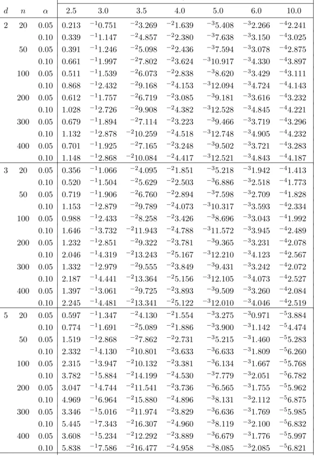
Upper quantiles of the null distribution of Tn,β have been approximated by gene-rating 100,000 samples from a law Nd(0,Id). Table 1 displays some critical values with the convention that an entry like−41.17 stands for 1.17×10⁻⁴. The results show that large sample sizes are required to approximate the critical values by their corresponding asymptotic values.
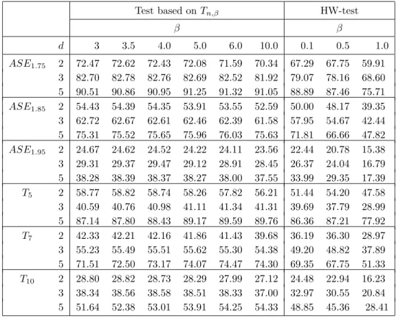
A natural competitor of the test based on Tn,β is the CF-based test studied in Henze and Wagner (1997) (HW-test). The latter procedure is simple to compute as well as affine invariant, and it has revealed good power performance with regard to competitors. The behaviour of the test based onTn,βin relation to the HW-test depends on whether the distribution is heavy-tailed or not. We tried a number of non-heavy-tailed distributions (specifically, the multivariate Laplace distribution, finite mixtures of normal distributions, the skew-normal distribution, the multivariateχ2-distribution, the Khintchine distribution, the uniform distribution on [0,1]d and the Pearson type II family). For these distributions we observed that the power of the proposed test is either similar or smaller than that of the HW-test; for very heavy-tailed distributions, the new test outperforms the HW-test. This observation can be appreciated by looking at Table 2, which displays the empirical power calculated by generating 10,000 samples (in each case), for the significance level α = 0.05, from the following heavy-tailed alternatives: (ASEθ) the θ-stable and elliptically-contoured distribution and the (Tθ) multivariate Student’s t with θ degrees of freedom. The same fact was also observed in Zghoul (2010), who numerically studied the test based onTn,β for univariate data.
In our simulations we tried a large number of values forβ for the proposed test as well as for the HW-test. The tables display the results for those values ofβ giving the highest power in most of the cases considered. The same can be said for the simulations
Table 1: Critical points for π−d/2T n,β. β d n α 2.5 3.0 3.5 4.0 5.0 6.0 10.0 2 20 0.05 0.213 −10.751 −23.269 −21.639 −35.408 −32.266 −42.241 0.10 0.339 −11.147 −24.857 −22.380 −37.638 −33.150 −43.025 50 0.05 0.391 −11.246 −25.098 −22.436 −37.594 −33.078 −42.875 0.10 0.661 −11.997 −27.802 −23.624 −310.917 −34.330 −43.897 100 0.05 0.511 −11.539 −26.073 −22.838 −38.620 −33.429 −43.111 0.10 0.868 −12.432 −29.168 −24.153 −312.094 −34.724 −44.143 200 0.05 0.612 −11.757 −26.719 −23.085 −39.181 −33.616 −43.232 0.10 1.028 −12.726 −29.908 −24.382 −312.528 −34.845 −44.221 300 0.05 0.679 −11.894 −27.114 −23.223 −39.466 −33.719 −43.296 0.10 1.132 −12.878 −210.259 −24.518 −312.748 −34.905 −44.232 400 0.05 0.701 −11.925 −27.165 −23.248 −39.502 −33.721 −43.283 0.10 1.148 −12.868 −210.084 −24.417 −312.521 −34.843 −44.187 3 20 0.05 0.356 −11.066 −24.095 −21.851 −35.218 −31.942 −41.413 0.10 0.520 −11.504 −25.629 −22.503 −36.886 −32.518 −41.773 50 0.05 0.719 −11.906 −26.760 −22.894 −37.598 −32.709 −41.828 0.10 1.153 −12.879 −29.789 −24.073 −310.317 −33.593 −42.334 100 0.05 0.988 −12.433 −28.258 −23.426 −38.696 −33.043 −41.992 0.10 1.646 −13.732 −211.943 −24.788 −311.572 −33.945 −42.489 200 0.05 1.232 −12.851 −29.322 −23.781 −39.365 −33.231 −42.078 0.10 2.046 −14.319 −213.243 −25.167 −312.210 −34.123 −42.567 300 0.05 1.332 −12.979 −29.555 −23.849 −39.431 −33.242 −42.072 0.10 2.187 −14.441 −213.364 −25.156 −312.105 −34.073 −42.527 400 0.05 1.397 −13.061 −29.725 −23.893 −39.509 −33.260 −42.084 0.10 2.245 −14.481 −213.341 −25.122 −312.010 −34.046 −42.519 5 20 0.05 0.597 −11.347 −24.130 −21.554 −33.275 −30.971 −53.884 0.10 0.774 −11.691 −25.089 −21.886 −33.900 −31.142 −54.474 50 0.05 1.519 −12.868 −27.862 −22.731 −35.215 −31.460 −55.283 0.10 2.332 −14.130 −210.801 −23.633 −36.633 −31.809 −56.260 100 0.05 2.315 −13.947 −210.132 −23.381 −36.134 −31.667 −55.768 0.10 3.782 −15.884 −214.199 −24.530 −37.779 −32.051 −56.782 200 0.05 3.047 −14.744 −211.541 −23.736 −36.565 −31.755 −55.962 0.10 4.969 −16.964 −215.880 −24.896 −38.131 −32.112 −56.875 300 0.05 3.346 −15.016 −211.974 −23.829 −36.636 −31.769 −55.985 0.10 5.445 −17.343 −216.307 −24.960 −38.119 −32.100 −56.832 400 0.05 3.608 −15.234 −212.292 −23.889 −36.679 −31.776 −55.997 0.10 5.838 −17.586 −216.477 −24.958 −38.085 −32.085 −56.821
Table 2: Percentage of rejection for nominal levelα = 0.05 and n= 50.
Test based onTn,β HW-test
β β d 3 3.5 4.0 5.0 6.0 10.0 0.1 0.5 1.0 ASE1.75 2 72.47 72.62 72.43 72.08 71.59 70.34 67.29 67.75 59.91 3 82.70 82.78 82.76 82.69 82.52 81.92 79.07 78.16 68.60 5 90.51 90.86 90.95 91.25 91.32 91.05 88.89 87.46 75.71 ASE1.85 2 54.43 54.39 54.35 53.91 53.55 52.59 50.00 48.17 39.35 3 62.72 62.67 62.61 62.46 62.39 61.58 57.95 54.67 42.44 5 75.31 75.52 75.65 75.96 76.03 75.63 71.81 66.66 47.82 ASE1.95 2 24.67 24.62 24.52 24.22 24.11 23.56 22.44 20.78 15.38 3 29.31 29.37 29.47 29.12 28.91 28.45 26.37 24.04 16.79 5 38.28 38.39 38.37 38.27 38.00 37.55 33.99 29.35 17.39 T5 2 58.77 58.82 58.74 58.26 57.82 56.21 51.44 54.20 47.58 3 40.59 40.76 40.98 41.11 41.34 41.31 39.69 37.79 28.99 5 87.14 87.80 88.43 89.17 89.59 89.76 86.36 87.21 77.92 T7 2 42.33 42.21 42.16 41.86 41.43 39.68 36.19 36.30 28.97 3 55.23 55.49 55.51 55.62 55.30 54.38 49.20 48.82 37.89 5 71.51 72.50 73.17 74.07 74.47 74.30 69.35 67.75 51.33 T10 2 28.80 28.82 28.73 28.29 27.99 27.12 24.48 22.94 16.23 3 38.34 38.56 38.58 38.51 38.33 37.00 32.97 30.55 20.84 5 51.64 52.38 53.01 53.91 54.25 54.33 48.85 45.36 28.41
in the next subsection.
6.2. Numerical experiments for GARCH data
In our simulations we considered a bivariate CCC–GARCH(1,1) model with
b= 0.1 0.1 , B1 = 0.1 0.1 0.1 0.1 , Γ1 = γ 0.01 0.01 γ , R= 1 r r 1 ,
for γ = 0.3,0.4,0.5 and r = 0,0.3, and a trivariate CCC–GARCH(1,1) model with
b= (0.1,0.1,0.1)0, B1 = 0.1 0.1 0.1 0.1 0.1 0.1 0.1 0.1 0.1 , Γ1 = γ 0.01 0.01 0.01 γ 0.01 0.01 0.01 γ , R= 1 r r r 1 r r r 1
and γ and r as before. The parameters in the CCC-GARCH models were estimated by their QMLE using the package ccgarch of the language R. For the distribution of the innovations, we tookε1, . . . , εni.i.d. from the distribution of εwithε having a (N) multivariate normal distribution, in order to study the level of the resulting bootstrap
test. To assess the power we considered the following heavy-tailed distributions: Tθ, the multivariateβ-generalized distribution (GNθ), that coincides with the normal dis-tribution for θ = 2 and has heavy tails for 0< θ <2 (Goodman and Kotz, 1973), and the asymmetric exponential power distribution (AEP), whereby (X1, . . . , Xd)>, with X1, . . . , Xd i.i.d. from a univariate AEP distribution (Zhu and Zinde-Walsh, 2009) with parameters α= 0.4, p1 = 1.182 and p2 = 1.820 (these settings gave useful results
in practical applications for the errors in GARCH type models). As in the previous subsection, we also calculated the HW-test.
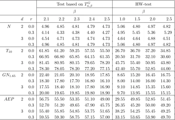
Table 3 reports the percentages of rejections for nominal significance levelα= 0.05 and sample size n = 300, for r = 0, 0.3 and γ = 0.4. The resulting pictures for
γ = 0.3, 0.5 are quite similar so, to save space, we omit the results for these values of
γ. In order to reduce the computational burden we adopted the warp-speed method of Giacomini et al. (2013), which works as follows: rather than computing critical points for each Monte Carlo sample, one resample is generated for each Monte Carlo sample, and the resampling test statistic is computed for that sample; then the resampling critical values forTG
n,β are computed from the empirical distribution determined by the resampling replications of Tn,βG∗. In our simulations we generated 10,000 Monte Carlo samples for the level and 2,000 for the power. Looking at Table 3, we conclude that: the actual level of the proposed bootstrap test is very close to the nominal level, and this is also true for the HW-test (although to the best of our knowledge, the consistency of the bootstrap null distribution estimator of the HW-test statistic has been proved only for the univariate case in Jim´enez-Gamero, 2014); and with respect to the power, the proposed test in most cases outperforms the HW-test.
6.3. A real data set application
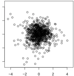
As an illustration, we consider the monthly log returns of IBM stock and the S&P 500 index from January 1926 to December 2008 with 888 observations. This data set was analyzed in Example 10.5 of Tsay(2010), where it is showed that a CCC-GARCH(1,1) model provides a adequate description of the data, which is available from the website http://faculty.chicagobooth.edu/ruey.tsay/teaching/fts/) of the author. We applied the proposed test and the HW test for testing H0,G. The p -values were obtained by generating 1000 bootstrap samples. For all -values of β in
Table 3: Percentage of rejections for nominal levelα= 0.05, γ = 0.4 and n= 300. Test based onTG n,β HW-test β β d r 2.1 2.2 2.3 2.4 2.5 1.0 1.5 2.0 2.5 N 2 0.0 4.96 4.85 4.81 4.79 4.73 5.06 4.80 4.97 4.82 0.3 4.14 4.33 4.38 4.40 4.27 4.95 5.45 5.36 5.29 3 0.0 4.54 4.71 4.73 4.74 4.73 4.64 4.64 4.88 4.51 0.3 4.96 4.85 4.81 4.79 4.73 5.06 4.80 4.97 4.82 T10 2 0.0 61.85 61.20 59.25 57.55 55.50 26.70 36.70 37.20 34.85 0.3 66.95 66.80 65.85 64.15 61.35 20.50 31.70 32.10 30.60 3 0.0 81.45 80.95 80.15 79.65 78.20 45.75 55.40 50.95 43.80 0.3 78.30 78.05 78.20 77.20 77.15 42.40 55.70 52.85 44.00 GN1.65 2 0.0 22.40 21.05 20.10 18.95 17.85 8.65 15.20 16.45 16.75 0.3 18.30 17.80 17.70 16.80 16.10 8.00 14.00 16.00 14.30 3 0.0 17.55 18.40 18.10 17.80 16.90 9.10 14.85 15.35 15.60 0.3 20.00 19.65 19.85 19.80 18.90 9.70 13.95 15.55 15.15 AEP 2 0.0 56.75 55.50 53.35 51.10 49.00 29.55 49.85 52.85 51.45 0.3 52.70 51.20 49.65 47.90 45.75 26.35 45.20 50.00 49.20 3 0.0 55.40 55.85 54.85 53.75 51.65 38.25 54.25 55.45 49.25 0.3 59.55 59.30 58.75 57.15 57.00 33.15 53.65 53.90 49.70
Table 3 we get the same p-value, 0.000, which leads us to reject H0,G, as expected by looking at Figure 1, which displays the scatter plot of the residuals after fitting a CCC-GARCH(1,1) model to the log returns, and Figure 2, that represents the histograms of the marginal residuals with the probability density function of a standard normal law superimposed.
7. Conclusions
We have studied a class of affine invariant tests for multivariate normality both in an i.i.d. setting and in the context of testing that the innovation distribution of a multivariate GARCH model is Gaussian, thus generalizing results of Henze and Koch (2017) in two ways. The test statistics are suitably weighted L2-statistics based on the difference between the empirical moment generating function of scaled residuals of the data and the moment generating function of the standard normal distribution in Rd. As such, they can be considered as ’moment generating function analogues’ to
● ● ● ● ● ● ● ● ● ● ●● ● ● ● ● ● ● ● ● ● ● ● ● ● ● ● ● ● ● ● ● ● ● ● ● ● ● ● ● ● ● ● ● ● ● ● ● ● ● ● ● ● ● ● ● ● ● ● ● ● ● ● ● ● ● ● ● ● ● ● ● ● ● ● ● ● ● ● ● ● ● ● ● ● ● ● ● ● ● ● ● ● ● ● ● ● ● ● ● ● ● ● ● ● ● ● ● ● ● ● ● ● ● ● ● ● ● ●● ● ● ● ● ● ● ● ●● ● ● ● ● ● ● ● ● ● ● ● ● ● ● ● ● ● ● ● ● ● ● ● ● ● ● ● ● ● ● ● ● ● ● ● ● ● ● ● ● ● ● ● ● ● ● ● ● ● ● ● ● ● ● ● ● ● ● ● ● ● ● ● ● ● ● ● ● ● ● ● ● ● ● ● ● ● ● ● ● ● ● ● ● ● ● ● ● ● ● ● ● ● ● ● ● ● ● ● ● ● ● ● ● ● ● ● ● ● ● ● ● ● ● ● ● ●● ● ● ●● ● ● ● ● ● ● ● ● ● ● ● ● ● ● ● ● ● ● ● ● ● ● ● ● ● ● ● ● ● ● ● ● ● ● ● ●● ● ● ● ● ● ● ● ● ● ● ● ● ● ● ● ● ● ● ● ● ● ● ● ● ● ● ● ● ● ● ● ● ● ● ● ● ● ● ● ●● ● ● ● ● ● ● ● ● ● ● ● ● ● ● ● ● ● ● ● ● ● ● ● ● ● ● ●● ● ● ● ● ● ● ● ● ● ● ● ● ● ● ● ● ● ● ● ● ● ● ●● ● ● ● ● ● ● ● ● ● ● ● ● ● ● ● ● ● ● ● ● ● ● ● ● ● ● ● ● ● ● ● ● ● ● ● ● ● ● ● ● ● ● ● ● ● ● ● ● ● ● ● ● ● ● ● ● ● ● ● ● ● ● ● ● ● ● ● ● ● ● ● ● ● ● ● ● ● ● ● ● ● ● ● ● ● ●● ● ● ● ● ● ● ● ● ● ● ● ● ● ● ● ● ● ●● ● ● ● ● ● ● ● ● ● ● ● ● ● ● ● ● ● ● ● ● ● ● ● ● ● ● ● ● ● ● ● ● ● ● ● ● ● ● ● ●● ● ● ● ● ● ● ● ● ● ● ● ● ● ● ● ● ● ● ● ● ● ● ● ● ● ● ● ●● ● ● ● ● ● ● ● ● ● ● ● ● ● ● ● ● ● ● ● ● ● ● ● ● ● ●● ● ● ● ● ● ● ● ●● ● ● ● ● ● ● ● ● ● ● ● ● ● ● ● ● ● ● ● ● ● ● ● ● ● ● ● ● ● ● ● ● ● ● ● ● ● ● ● ● ● ● ● ● ● ● ● ● ● ● ● ● ● ● ● ● ● ● ● ● ● ● ● ● ● ● ● ● ● ● ● ●● ● ● ● ● ● ● ● ● ● ● ● ● ● ● ● ● ● ● ● ●● ● ● ● ● ● ● ● ● ● ● ● ● ● ● ● ● ● ●● ● ● ● ● ● ● ● ● ● ● ● ● ● ● ● ● ● ● ● ● ● ● ● ● ● ● ● ● ● ● ● ● ● ● ● ● ● ● ● ● ● ●● ● ● ● ● ● ● ● ● ● ● ● ● ● ● ● ● ● ● ● ● ● ● ● ● ● ● ● ● ● ● ● ● ● ● ● ● ● ● ● ● ● ● ● ● ● ● ● ● ● ● ● ● ● ● ● ● ● ● ● ● ● ● ● ● ● ● ● ● ● ● ● ● ● ● ● ● ● ● ● ● ● ● ● ● ● ● ● ● ● ● ● ● ● ● ●● ● ● ● ● ● ● ● ● ● ● ● ● ● ● ● ● ● ● ● ● ● ● ● ● ● ● ● ●● ●● ● ● ● ● ● ● ● ● ● ● ● ● −4 −2 0 2 4 −4 −2 0 2 4 IBM returns S&P500 retur ns
Figure 1: Scatter plot of the residuals.
IBM returns −4 −2 0 2 4 0.0 0.1 0.2 0.3 0.4 S&P500 returns −6 −4 −2 0 2 4 0.0 0.1 0.2 0.3 0.4
the time-honored class of BHEP tests that use the empirical characteristic function. As the decay of a weight function figuring in the test statistic tends to infinity, the test statistic approaches a certain linear combination of two well-known measures of multivariate skewness. The tests are easy to implement, and they turn out to be consistent against a wide range of alternatives. In contrast to a recently studied L2 -statistic of Henze et al. (2017) that uses both the empirical moment generating and the empirical characteristic function, our test is also feasible for larger sample sizes since the computational complexity is of orderO(n2). Regarding power, the new tests outperform the BHEP-tests against heavy-tailed distributions.
Acknowledgements
M.D. Jim´enez-Gamero was partially supported by grant MTM2014-55966-P of the Spanish Ministry of Economy and Competitiveness.
References
Arcones, M. (2007), Two tests for multivariate normality based on the characteristic function, Math. Methods Statist.,16, 177–201.
Bardet, J. M. and Wintenberger, O. (2009), Asymptotic normality of the quasi-maximum likelihood estimator for multidimensional causal processes, Ann. Statist., 37, 2730– 2759.
Baringhaus, L., and Henze, N. (1988), A consistent test for multivariate normality based on the empirical characteristic function,Metrika,35, 339–348.
Baringhaus, L., Ebner, B., and Henze, N. (2017), The limit distribution of weighted L2 -goodness-of fit statistics under fixed alternatives, with applications, Ann. Inst. Stat. Math.,69, 969–995.
Batsidis, A., Martin, N., Pardo, L., and Zografos, K. (2013), A necessary power divergence type family of tests for multivariate normality,Comm. Statist. – Simul. Comput.,42, 2253–2271.
Billingsley, P. (1968), Convergence of Probability Measures. John Wiley & Sons, New York-London-Sidney.
Bollerslev, T. (1990), Modelling the coherence in short-run nominal exchange rates: a multi-variate generalized ARCH model, Rev. Econ. Stat.,72, 498–505.
Bosq, D. (2000), Linear Processes in Function Spaces. Springer, New York.
Burke M.D. (2000), Multivariate tests-of-fit and uniform confidence bands using a weighted bootstrap,Statist. Probab. Lett.,46, 13–20.
Cardoso de Oliveira, I.R., and Ferreira, D.F. (2010), Multivariate extension of chi-squared univariate normality test, J. Statist. Comput. Simul.,80, 513–526.
Comte, F. and Lieberman, O. (2003), Asymptotic theory for multivariate GARCH processes, J. Multiv. Anal.,84, 61–84.
Cs¨org˝o, S. (1989), Consistency of some tests for multivariate normality,Metrika,36, 107–116. Eaton, M.L., and Perlman, M.D. (1973), The non-singularity of generalized sample covariance
matrices,Ann. Statist.,1, 710–717.
Ebner, B. (2012), Asymptotic theory for the tests of multivariate normality by Cox and Small, J. Multiv. Anal.,111, 368–379.
Enomoto, R., Okamoto, N., and Seo, T. (2012) Multivariate normality test using Srivastava’s skewness and kurtosis,SUT J. Math.,48, 103–115.
Farrel, P.J., Salibian–Barrera, M., and Naczk, K. (2007) On tests for multivariate normality and associated simulation studies,J. Statist. Comput. Simul.,77, 1053–1068.
Francq, C., Jim´enez-Gamero, M.D., and Meintanis, S.G. (2017), Tests for sphericity in mul-tivariate GARCH models, J. Econometrics,196, 305–319.
Francq, C. and Zako¨ıan, J.M. (2010), GARCH Models: Structure, Statistical Inference and Applications. Wiley, London.
Francq, C. and Zako¨ıan, J.M. (2012), QML estimation of a class of multivariate asymmetric GARCH models, Econometric Theory,28, 179–206.
Ghoudi K., and R´emillard, B. (2014), Comparison of specification tests for GARCH models, Computat. Statist. Data Anal.,76, 291–300.
Giacomini, R., Politis, D.N., and White, H. (2013), A warp-speed method for conducting Monte Carlo experiments involving bootstrap estimators, Econometric Theory, 29, 567–589.
Goodman, I.R., Kotz, S. (1973), Multivariate θ-generalized normal distributions, J. Multiv. Anal.,3, 204–219.
Hanusz, Z., and Tarasi´nska, J. (2008), A note on Srivastava and Hui’s test of multivariate normality, J. Multiv. Anal.,99, 2364–2367.
Hanusz, Z., and Tarasi´nska, J. (2012). New test for multivariate normality based on Small’s and Srivastava’s graphical methods,J. Statist. Comput. Simul.,82, 1743–1752.
Henze, N. (1997), Extreme smoothing and testing for multivariate normality,Statist. Probab. Lett.,35, 203–213.
Henze, N. (2002), Invariant tests for multivariate normality: a critical review,Statist. Papers,
43, 467–506.
Henze, N., Jim´enez-Gamero, M.D., and Meintanis, S.G. (2017), Characterizations of multinormality and and corresponding tests of fit, including for Garch models, arXiv:1706.03029.
Henze, N., and Koch, S. (2017), On a test of normality based on the empirical moment generating function,Statist. Papers, doi:10.1007/s00362-017-0923-7.
Henze, N., and Wagner, T. (1997), A new approach to the BHEP tests for multivariate normality, J. Multiv. Anal.,62, 1–23.
Henze, N., and Zirkler, B. (1990), A class of invariant consistent tests for multivariate nor-mality,Comm. Statist. Theory Methods,19, 3595–3617.
Jeantheau, T. (1998), Strong consistency of estimators for multivariate ARCH models, Econo-metric Theory,14, 70–86.
Jim´enez-Gamero, M.D. (2014), On the empirical characteristic function process of the resid-uals in GARCH models and applications,TEST,23, 409–432.
Jim´enez-Gamero, M.D., and Pardo-Fern´andez, J.C. (2017), Empirical characteristic function tests for GARCH innovation distribution using multipliers, J. Stat. Comput. Simul.,
87, 2069–2093.
Joenssen, D.W., and Vogel, J. (2014), A power study of goodness-of-fit tests for multivariate normality implemented in R,J. Stat. Comput. Simul.,84, 1055–1078.
J¨onsson, K., (2011), A robust test for multivariate normality, Econom. Lett.,113, 199–201. Kim, N. (2016), A robustified Jarque–Bera test for multivariate normality, Econom. Lett.,
140, 48–52,
Klar, B., Lindner, F. and Meintanis, S.G. (2012), Specification tests for the error distribution in GARCH models,Comput. Statist. Data Anal.,56, 3587–3598.
Koizumi, K., Hyodo, M., and Pavlenko, T. (2014), Modified Jarque–Bera tests for multivari-ate normality in a high-dimensional framework,J. Statist. Th. Pract.,8, 382–399. Mardia, K.V. (1970), Measures of multivariate skewness and kurtosis with applications,
Mecklin, Ch. J., and Mundfrom, D.J. (2005), A Monte Carlo comparison of the type I and type II error rates of tests of multivariate normality, J. Statist. Comput. Simul., 75, 93–107.
M´ori, T.F., Rohatgi, V.K., and Sz´ekely, G.J. (1993), On multivariate skewness and kurtosis, Theory Probab. Appl.38, 547–551.
Pudelko, J. (2005), On a new affine invariant and consistent test for multivariate normality, Probab. Math. Statist.,25, 43–54.
Rydberg, T.H. (2000), Realistic statistical modelling of financial data, Int. Stat. Rev., 68, 233–258.
Shorack, G. R., and Wellner, J. A. (1986),Empirical processes with applications to statistics, Wiley Series in Probability and Mathematical Statistics. John Wiley & Sons, Inc., New York, 1986.
Spierdijk, L. (2016), Confidence intervals for ARMA-GARCH Value-at-Risk: The case of heavy tails and skewness,Computat. Statist. Data Anal.,100, 545–559.
Sz´ekeley, G.J., and Rizzo, M.L. (2005), A new test for multivariate normality, J. Multiv. Anal.,93, 58–80.
Tenreiro, C. (2011), An affine invariant multiple test procedure for assessing multivariate normality, Comput. Statist. Data Anal.,55, 1980–1992.
Tenreiro, C. (2017), A new test for multivariate normality by combining extreme and nonex-treme BHEP tests, Commun. Statist. –Th. Meth.,46, 1746–1759.
Thulin, M. (2014), Tests for multivariate normality based on canonical correlations, Stat. Meth. Appl.,23, 189–208.
Tsay, R.S. (2010). Analysis of Financial Time Series. Wiley, Hoboken, New Jersey.
Villase˜nor-Alva, J.A., and Estrada, E.G. (2009), A generalization of Shapiro–Wilk’s test for multivariate normality,Commun. Statist. – Th. Meth.,38, 1870–1883.
Voinov, V., Pya, N., Makarov, R. and Voinov, Y. (2016), New invariant and consistent chi-squared type goodness-of-fit tests for multivariate normality and a related comparative simulation study, Commun. Statist. – Th. Meth.45, 3249–3263.
Yanada, T., Romer, M.M., and Richards, D. St. P. (2015), Kurtosis tests for multivariate normality with monotone incomplete data, TEST24, 532–557.
Zghoul, A.A. (2010), A goodness-of-fit test for normality based on the empirical moment generating function,Comm. Statist. – Simul. Comput.,39, 1292–1304.
Zhou, S., and Shao, Y. (2014), A powerful test for multivariate normality, J. Appl. Statist.,
41, 351–363.
Zhu, D., and Zinde-Walsh, V. (2009), Properties and estimation of asymmetric exponential power distribution. J. Econometrics, 148, 86–99.