A software-defined receiver for laser communications using a GPU

A Software-Defined Receiver for Laser

Communications Using A GPU

by

Joseph Matthew Kusters

Submitted to the Department of Electrical Engineering and Computer

Science

in partial fulfillment of the requirements for the degree of

Masters of Engineering in Electrical Engineering and Computer Science

at the

MASSACHUSETTS INSTITUTE OF TECHNOLOGY

September 2018

c

○

Massachusetts Institute of Technology 2018. All rights reserved.

Author . . . .

Department of Electrical Engineering and Computer Science

September 10, 2018

Certified by . . . .

Kerri L. Cahoy

Associate Professor

Thesis Supervisor

Accepted by . . . .

Katrina LaCurts

Chairman, Masters of Engineering Thesis Committee

A Software-Defined Receiver for Laser Communications Using

A GPU

by

Joseph Matthew Kusters

Submitted to the Department of Electrical Engineering and Computer Science on September 10, 2018, in partial fulfillment of the

requirements for the degree of

Masters of Engineering in Electrical Engineering and Computer Science

Abstract

Laser communication systems provide a high data rate, power efficient communi-cation solution for small satellites and deep space missions. One challenge that limits the widespread use of laser communication systems is the lack of accessible, low-complexity receiver electronics and software implementations. Graphics Process-ing Units (GPUs) can reduce the complexity in receiver design since GPUs require less specialized knowledge and can enable faster development times than Field Pro-grammable Gate Array (FPGA) implementations, while still retaining comparable data throughputs via parallelization. This thesis explores the use of a Graphics Pro-cessing Unit (GPU) as the sole computational unit for the signal proPro-cessing algorithms involved in laser communications.

Thesis Supervisor: Kerri L. Cahoy Title: Associate Professor

Acknowledgments

I would like to thank my advisor, Kerri Cahoy, for all of the help and opportunities she has given me. Her knowledge, work ethic, and leadership are out of this world and the research group she has created and shepherded is truly special. I would not be where I am today without her, doing what I love, surrounded by an extraordinary group of human beings.

I would like to thank my colleagues and mentors from along the way. Steven Leeb at MIT, Ryan Rogalin at JPL, and Rodrigo, Caleb, and Kit from STAR Lab were all critical in their own ways.

My friends deserve a special mention, for making Boston a city worth staying in and putting up with me when I’m completely zonked from school.

A final thanks goes to my family. My parents have always encouraged curiosity and deserve all of the blame for why I enjoy school so much. From weekends at the Natural History Museum and the Zoo, to late nights and phone calls helping me with school, the support and love they provided is incredible. My brother too, for being a sounding board and confidant for anything and everything.

Contents

1 Introduction 13

1.1 CubeSats and Optical Communication . . . 13

1.2 Motivation for software receivers . . . 15

1.3 Current Ground Station Performance . . . 16

1.3.1 Lunar Laser Communication Demonstration . . . 16

1.3.2 Optical Communication and Sensor Demonstration . . . 17

1.4 Metrics . . . 17 1.5 Thesis Organization . . . 18 2 Background 19 2.1 Detection . . . 19 2.2 Hardware . . . 20 2.2.1 Detector . . . 20 2.2.2 Sampling . . . 21 2.2.3 Sample Piping . . . 21

2.3 Signal Processing Algorithms . . . 22

2.3.1 Clock Recovery . . . 22

2.3.2 Forward Error Correction . . . 24

3 Methods Developed 29 3.1 GPU Preliminaries . . . 29

3.2 Channel Model . . . 30

3.3.1 ISGT Maximum Likelihood Slot Synchronization . . . 30

3.3.2 MF/FAS Frame Synchronization . . . 31

3.3.3 Log-Likelihood Ratios . . . 32

3.4 Demodulation and Decoding . . . 32

3.4.1 Code Design . . . 33

3.4.2 Inference on Tanner Graph . . . 33

3.4.3 Node Calculations and Approximations . . . 34

3.4.4 Parallel Node Implementation . . . 36

4 Results 37 4.1 Slot Synchronization . . . 37 4.2 Frame Synchronization . . . 38 4.3 LLR Generation . . . 39 4.4 Decoding . . . 40 5 Summary 41 5.1 Conclusions . . . 41 5.2 Future Work . . . 41

List of Figures

2-1 Received PPM Pulses over 5 Symbols . . . 23

2-2 Aggregated PPM Pulses over 100 Symbols . . . 23

3-1 Aggregate Slots with an offset of 3.5 . . . 31

3-2 Aggregate Slots After Shifting . . . 31

3-3 Example of a Tanner Graph, variable nodes represent LLRs of trans-mitted bits, check nodes represent parity constraints dictating the up-date rule . . . 33

List of Tables

1.1 Recent Optical Ground Station Performance . . . 16 4.1 Slot Synchronization Performance, M = 16, n = 3000, N = 100

aver-aged over 30 runs. . . 38 4.2 Frame Synchronization Performance, M=16, n =3000, N= 17

aver-aged over 30 runs . . . 39 4.3 LLR Generation Performance, M= 16, n= 3000, averaged over 30 runs 40 4.4 Decoding Performance, M= 16, n =3000, averaged over 30 runs . . 40

Chapter 1

Introduction

Software receivers are significantly easier to build in terms of time and cost compared to FPGA or hardware receivers, and offer increased flexibility and ease of upgrading. Using graphics processing units (GPUs) to increase the processing speed with only small increases in system complexity is an attractive solution to meeting the high data rate needs of modern spacecraft missions.

1.1

CubeSats and Optical Communication

Electronics today continue to get smaller and faster as Moore’s Law and the Inter-net afford us the ever-increasing ability to connect to anyone and anywhere. The improved electronics capabilities are of particular benefit to the space community, as the decreased size, weight, and power needs of electronics allow for nanosatel-lites (also known as CubeSats), originally proposed by university researchers [31], to perform missions previously developed by government agencies and industry with budgets of up to hundreds of millions of dollars per projects. Space is more accessible for nanosatellites, and their new capabilities enabled by early adoption of commer-cial technologies result in more ambitious projects. As these projects take on more data-intensive instruments, communications becomes a limiting factor.

Traditional satellites, both large and small, have used radio communications to talk with ground operators. Although optical communications has been demonstrated

from larger space platforms [8] [3], in comparison to optical communication, radio is much easier to point, due to radio’s wider beamwidth, and typical radios are easier to design and build, due to decades of heritage research and development. However, it is challenging to achieve high data rates on nanosatellites due to the lack of available volume and power. Achieving high data rates on nanosatellites is challenging using radio due to the wider beamwidth, as radio systems require a larger antenna or array of elements to achieve high gain, or require more power as the signal is less directed to the receiver. In addition, the radio frequency available bandwidth is highly contested, and systems must comply with sometimes complex regulations to avoid interference. The size, weight, and power (SWaP) constraints on nanosatellites (CubeSats) along with the need for low-cost solutions, make it difficult to significantly increase data rates using radio frequency communications. This is especially true if using com-mercial off-the-shelf (CotS) parts, which most CubeSats baseline to reduce cost and development time. As the amount of data generated by nanosatellites has increased, close to the theoretical limit (the Shannon limit) is the limit for radio communication systems, emphasizing constraints due to regulatory bandwidth restrictions.

Laser communications (lasercom, or free space optical) can increase the data rates available to nanosatellites. Because of the larger available bandwidth for lasercom, and the improved power efficiency if a narrow beam is used, lasercom links have higher capacity in comparison to radio [11].

There are still challenges that need to be overcome in implementing lasercom on nanosatellites. Pointing requirements are significantly harder to achieve, but recent developments in nanosatellite attitude determination and control systems, and the introduction of staged control systems at nanosatellite scale have made it possible for nanosatellites to point accurately enough for laser communication to be viable [11] [26] [45].

Ground stations are also a problem, as the infrastructure to easily downlink laser-com data with a variety of bands, modulation and coding types, and geographic locations does not yet exist. The work done by Riesing, et al. on the Portable Telescope for Lasercom (PorTeL) [35] has demonstrated the feasibility of using

com-mercially available telescopes to meet this need. To date, not as much attention has been paid to tailoring the signal processing algorithms to optical communications and using commercially available processing capability.

Many lasercom receiver designs use older algorithms, such as Serially Concate-nated Convolutional Codes on the Lunar Lasercom Demonstration (LLCD) and the Deep Space Optical Communications project (DSOC) [29] or Reed-Solomon (NODE) [46] with Interleaving, which either limit the data rate achievable due to their com-plexity, have limits on parallelizing, or are non-optimal. To fully take advantage of the benefits of optical communication, receivers must be tailored to the use case.

1.2

Motivation for software receivers

Field Programmable Gate Arrays (FPGAs) are the current norm in communications electronics, with their high parallel processing power well-suited for digital signal processing (DSP) algorithms. They require specialized engineers, however, to build customized digital circuits through programming languages specific to FPGAs such as VHDL, and the development times are longer compared to traditional software projects, due to individual iterations needing more time (compilation takes longer, and hardware being harder to debug due to obfuscation). Software receivers, where all of the DSP is done on a CPU in a traditional programming language, eliminate these two problems, as traditional programming is a more prevalent skill among engineers, requiring less specialized electronics knowledge, and rapid iterations are more feasible. Software receiver implementations, however, suffer from the loss of parallel processing compared with FPGAs, and therefore are not capable of the same speeds as FPGA receivers, even though CPUs run serially much faster than FPGAs.

Graphics Processing Units (GPUs) offer a solution to this problem, with their parallel processing and serial speed occupying a middle ground between CPUs and FPGAs. GPUs can support the same rapid iterations as in CPU development and only require slightly more specialized knowledge to program than a CPU, something any engineer familiar with C programming can pick up quickly. This thesis focuses on

investigating how compelling the benefits of using a GPU for lasercom receivers are, and whether GPU-based software receivers can compete with FPGA-based receivers for use in optical communications terminals.

1.3

Current Ground Station Performance

An overview of recent lasercom missions and their ground stations can be found in [35]. The rest of this section will discuss two specific missions, the Lunar Laser Communication Demonstration (LLCD) and the Optical Communication and Sensor Demonstration (OCSD), and the relevant receiver algorithms and metrics they used.

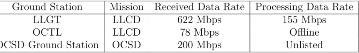
Table 1.1: Recent Optical Ground Station Performance

Ground Station Mission Received Data Rate Processing Data Rate

LLGT LLCD 622 Mbps 155 Mbps

OCTL LLCD 78 Mbps Offline

OCSD Ground Station OCSD 200 Mbps Unlisted

1.3.1

Lunar Laser Communication Demonstration

LLCD was a lasercom demonstration payload on the LADEE (Lunar Atmosphere and Dust Environment Explorer) orbiter. The LLCD lasercom system development was led by MIT Lincoln Laboratory in 2013 which demonstrated a 622 Mbps laser-com downlink from the Moon to Earth [30]. NASA Jet Propulsion Laboratory also supported LLCD.

The LLCD mission made use of optical Frame Acquisition Sequences and Inter-Symbol Guard Times for clock recovery and Serially Concatenated Pulse Position Modulation for forward error correction and modulation [44], which are discussed in more detail in Chapters 2 and 3. For the Lunar Lasercom Ground Terminal (LLGT) developed at Lincoln Labs for LLCD [8], with these methods, processing at the receiver was initially only capable of throughput of up to 155 Mbps. Additional FPGAs had to be added to reach 622 Mbps [43]. The bottleneck on the processing speed is the computationally intense decoding algorithm, with performance being

constrained by the serial nature of decoding SCPPM [43]. SCPPM is used in spite of this limitation, due to its strong error correcting capabilities [29].

An alternate ground terminal to the LLGT was the Optical Communications Telescope Laboratory (OCTL) developed at JPL [7]. OCTL only supported data rates up to 78 Mbps due to pointing and acquisition constraints, and all of the signal processing was done offline, highlighting the difficulty of designing and implementing electronics and software that can process lasercom signals even at lower data rates of 78 Mbps.

1.3.2

Optical Communication and Sensor Demonstration

OCSD is a mission developed by The Aerospace Corporation, capable of demonstrat-ing 50-200 Mbps from low Earth orbit to ground. The transmitter may be capable of higher data rates, but the mission data rate may be limited by the receiver electronics available [37]. This highlights the need for receiver designs capable of scaling to above 1 Gbps.

1.4

Metrics

The relevant metrics for a GPU-based software receiver focus on information theoretic properties and actual data throughput. The information theoretic metric of relevance is channel capacity and the gap to capacity of the given forward error correction code. For real communications systems, the throughput of the signal processing algorithms matters, as this constrains the actual data rate seen by the decision making system. Throughput derives from both the computational complexity of the algorithms in-volved, and how parallelizable an algorithm is. Parallelization is the primary means of increasing throughput as Moore’s law slows down, because it becomes increasingly challenging to add transistors to CPUs, and thermal and power constraints prevent CPUs from increasing clock speeds to improve serial computation power. This is one of the reasons why FPGAs and GPUs are starting to outperform traditional CPUs for given applications, such as in digital signal processing, image processing and machine

learning [38] [5] [41].

1.5

Thesis Organization

Chapter 2 details the status of current receiver architectures and methods, and iden-tifies research and performance gaps. Chapter 3 describes the approach to designing a software lasercom receiver for a GPU. Algorithm implementations for clock recov-ery and decoding, are detailed. Chapter 4 discusses the performance results of the receiver implementation. Comparisons are made with modern receiver implemen-tations. Chapter 5 summarizes the work done for this thesis and discusses future work.

Chapter 2

Background

Communications systems can be divided into three blocks, a transmitter, a channel, and a receiver. This thesis focuses on receiver design, which concerns itself with the channel only as far as creating a model from which signal distortion (noise charac-teristics) can be calculated and used in the signal processing algorithms. It is well documented that the optical communication channel with Pulse Position Modulation [21] [18] [9] can be modeled as an m-ary Poisson Channel.

There are a variety of resources that detail the design and analysis of lasercom systems. Gagliardi and Karp [18] go over the physics of optical signals, direct and coherent detection, modulation and encoding techniques, and use specific examples from fiber optic, terrestrial, and space channels. Hemmati has similar texts [20] [21] which specifically focuses on lasercom systems for the deep space channel. For a detailed discussion on the tradeoffs in detection and modulation schemes used in photon-starved systems, Caplan has an excellent chapter in his book [9].

2.1

Detection

The optical communication channel can make use of two broad forms of detection, either coherent, where the data is modulated onto the phase of the signal, or direct, where the data is modulated onto the amplitude of the signal. In direct detection, photon counts are calculated from the electrical signal out of a detector as it responds

to the optical signal. This form of detection lends itself to amplitude modulation tech-niques, such as On Off Keying (OOK) or Pulse Position Modulation. In Pulse Position Modulation, a data symbol is divided into M slots (referred to as the PPM order, or M), and one pulse is sent per symbol in one of these slots. The data transmitted is then demodulated as a number between 0 and M-1, corresponding directly to the slot the pulse was sent in. The tradeoffs between direct detection versus coherent detection are about power efficiency and spectral efficiency. Amplitude modulation is more power efficient and less complex to implement, while phase modulation tech-niques have a higher spectral efficiency (higher data rate for a given communication bandwidth), but require more power and complexity [9]. Amplitude modulation and direct detection are the schemes discussed in this thesis for nanosatellites and deep space links due to the power constraints of these missions.

2.2

Hardware

2.2.1

Detector

In order to do direct detection, a detector is needed which produces an electrical re-sponse to a received optical signal. Two examples are Avalanche Photodiodes (APDs) and Superconducting Nanowire Single Photon Detectors (SNSPDs). SNSPDs are used for deep space links as they are capable of detecting individual photons, which is necessary for the low photon regime of deep space optical communications. They require a specialized thermal control system to keep the detector in the supercon-ducting regime, and complex electronics for photon detection. This makes them expensive, and while suitable for deep space missions, they are not likely to be used for nanosatellite missions.

For nanosatellite missions, APDs are more suitable. They can be bought com-mercially at relatively low cost, coming in packages complete with biasing electronics. A high-speed Analog-to-Digital Converter (ADC) is the only circuit needed for sam-pling outside of the electronics to bias the APD. The semiconductor used for the APD

dictates the optical wavelength it responds to, such as Indium Gallium Arsenide (In-GaAs) for 800-2600 nm, Germanium for 400-1700 nm, and Silicon for 190-1100 nm. As APDs are made out of normal semiconductor material, their operating temper-atures are comparable to other commercial electronics and therefore do not require any specialized thermal control.

2.2.2

Sampling

Both the APD and SNSPD electrical responses can be used to produce the photon counts needed for the PPM signal. The SNSPD uses the digital circuit discussed in [16]. An APD can be sampled using either a Time-to-Digital Converter (TDC) or an ADC. The advantage of an ADC is you can choose between working with photon counts or electrical signals in the signal processing algorithms [9]. The signal processing algorithms in this thesis use photon counts, but transitioning between photon counts and voltage samples is only a matter of changing channel models (Gaussian versus Poisson), and has a negligible impact on the complexity of the calculations involved [9] [21] [18].

2.2.3

Sample Piping

Moving the samples from the detector to processor memory requires high-speed digital interfaces. These are usually Low-Voltage Differential Signaling (LVDS) or Current Mode Logic (CML) outputs, defined by such standards as JESD204B [1]. In order to use these interfaces, specialized ICs or FPGAs are required, as GPUs and CPUs do not contain the necessary interface components. Peripheral Component Interconnect Express (PCIe) is the only standard interface for GPUs and CPUs that can move data at the required rate for lasercom, but there are no sampling chips which have this interface. A more detailed study is needed to find an optimal design for piping samples from the detector into processor memory.

2.3

Signal Processing Algorithms

With the photon counts now in digital form, the original data needs to be recovered. To accurately do this for PPM, the transmit clock must be recovered and used to synchronize the received slots with the transmitted, and the the received bits need to be demodulated and decoded. This is done using a variety of algorithms, broken up into two broad categories, clock recovery and forward error correction.

2.3.1

Clock Recovery

In order to accurately demodulate and decode the PPM signal, it needs to be known in which of M slots a given pulse was sent (slot synchronization) and where code-words begin and end (frame synchronization). The transmitter clock will have some variation, referred to as clock jitter, and there will be some offset between when a slot is sampled on the receiver and when that slot was actually sent from the trans-mitter. This is referred to as the slot offset, and the algorithms for estimating it are referred to as slot synchronization. This is in contrast to the estimation of the beginning and ending of codewords, which is referred to as the frame offset and frame synchronization respectively.

Slot synchronization can be achieved using a few different approaches [36] [32] [44], but the primary method is using Intersymbol Guard Times (ISGTs). A certain number of slots are left blank; a pulse is never transmitted in these slots. This number can vary depending on the Signal-to-Noise Ratio (SNR), but a good rule of thumb is one-fourth the PPM order. This reduces the data rate for a given slot clock by 20 percent, but allows accurate calculation of the slot offset. With these blank slots, over the course of enough symbols, these slots become obvious as depicted in Figure 2-1 and 2-2. The slot counts can then be combined into aggregate slot counts over a given number of symbols, large enough to make the guard slots obvious, but not large enough so as to make the clock jitter affect the estimate accuracy. A simple approach to calculating the offset would be to take these aggregate slot counts, find the minimum sum of continuous slot counts over a window the size of the guard

Figure 2-1: Received PPM Pulses over 5 Symbols

Figure 2-2: Aggregated PPM Pulses over 100 Symbols

time, and call this the integer offset. Then, estimate the average signal count and noise count for the slots and use this to estimate the fractional slot offset. This leads to inaccuracies due to the random nature of the channel, which can be mitigated if we use our knowledge of the channel statistics for a more sophisticated estimation scheme. From the Poisson PPM channel, the signal counts and noise counts obey a Poisson distribution and a maximum-likelihood estimator was derived and tested by JPL [36]. It approaches the Cramer-Rao bound quickly, and can therefore be used on a small enough sample size to avoid the hazards of clock jitter.

Frame synchronization requires a different approach. A header, or Frame Acquisi-tion Sequence (FAS), is transmitted at the start of every codeword [17]. This specific bit sequence can be accurately detected then using a Matched Filter approach at the receiver. The known bit sequence translates to known signal shape, which is stored on the receiver and then an autocorrelation is calculated across a codeword (also referred to as frame). Once the peak is found, the frame offset is calculated and used to align codewords for the decoder. As a maximum-likelihood approach with ISGTs is used to find any fractional offset on the slots, and the slot clock is aligned as a result, only the integer symbol offset is needed from the autocorrelation.

The frame synchronization consists of an autocorrelation done n times, where n is the frame length (the block length, length of a codeword) plus the length of the FAS. Each of these autocorrelations does not depend on the others, and therefore all can be calculated at the same time. The frame length for space communications is about a few thousand in the longest cases [10] [21], and this is on the order of how many parallel threads can be spun up on modern GPUs [2]. This implies throughput performance should be similar to FPGA-based approaches, if not faster, as FPGA implementations derive their high throughputs based on massive parallelization. Slot synchronization is a similar story, with the number of PPM symbols for an accurate estimate presented in detail in Chapter 4.

2.3.2

Forward Error Correction

The forward error correction (FEC) portion of the receiver concerns itself with recov-ering the original information the transmitter was trying to send. The field of FEC, also referred to as channel coding, began with Shannon’s 1948 paper that created the field of information theory [39], in which he detailed the optimal method for both encoding transmitted information and decoding received information so as to achieve error free data transmission. The methods Shannon described are usually computa-tionally infeasible for real systems to use, and since 1948 a large variety of methods have been developed that are practical for use but may not reach this maximum error free rate of transmission, called the Shannon limit, or channel capacity.

For lasercom, the two methods that have been widely used are Reed-Solomon codes and a class of turbo codes called Serially-Concatenated Convolutional Codes (SCCC) combined with a PPM modulator to produce SCPPM [29] [10] [21] [46]. Both of these approaches also make use of interleaving to deal with burst errors in the atmospheric fading channel [21]. A third class of codes, Low-Density Parity Check (LDPC) codes, have also been proposed [21] [15] and recent work tailoring them to lasercom has shown promise [28]. Detailed background on LDPC codes and Turbo codes, and the iterative decoding of them, is given in Urbanke and Richardson’s textbook [34] and Mackay’s textbook [27].

Reed-Solomon (RS) codes are a widely used class of FEC codes, due to their high minimum codeword distance and low complexity encoding and decoding operations [21]. Their application to lasercom has been studied, and Reed-Solomon Pulse Po-sition Modulation (RS-PPM) performs within a few decibels (dB) of capacity for the Poisson PPM channel [21]. This can be a favorable coding scheme for missions looking to minimize system complexity, not having high data downlink requirements, and operating in a high SNR regime. To fully take advantage of lasercom attributes, though, a coding scheme which approaches capacity must be used, which is where SCPPM comes in.

SCPPM was designed at JPL, first proposed in 2005 [29] as a means of getting close to capacity for a deep space link. It operates using the turbo principle first discovered in the 1990s [6], which found that by combining two convolutional codes and a bit interleaver, a code could be designed which arbitrarily approached capac-ity using an iterative decoder. Using this, SCPPM is able to get within ∼1 dB of capacity, compared to the ∼3 dB of capacity of RS-PPM [29] [21]. SCPPM trades this improved error performance for increased computational complexity, using the Bahl-Cocke-Jelinek-Raviv (BCJR) algorithm for decoding, which operates on a Trel-lis graph data structure. This breaks the decoder into an inner and an outer decoder, with LLRs being updated in one and then passed to the other in a step, then the reverse happening in the second step of an iteration, with iterations continuing until some stopping condition is reached. The individual decoders within the BCJR decoder are for the individual codes concatenated together to make SCPPM, a convolutional code and a 1/(1+D) accumulator concatenated with a PPM symbol mapper. This PPM symbol mapper is how the SCPPM code combines the decoding and demodu-lation into the same step. This also results in improved performance, as there is no information loss between demodulation and decoding, as hard decisions are not made in order to break up PPM symbols, keeping all of the information associated with the original channel observation.

Both the inner and outer decoders are recursive in nature, as the update rule relies on the previous step of the update rule in the decoders, minimizing the gains to

be made from parallel computation. Pipelining provides a means of speeding up the decoder, but this implementation requires an FPGA for use, and to get reasonable speeds, multiple FPGAs have to be used, as in the LLCD ground terminal which used 5 separate FPGAs for the decoder to reach throughputs of 155 Mbps [43]. An additional interleaver outside of the one within the SCPPM code also must be used to account for longer fades associated with the atmospheric downlink channel.

LDPC codes are a possible competitor with SCPPM to achieve near capacity per-formance. They were originally developed in 1963 in Gallagher’s PhD thesis [19], in which he also proposed the Belief Propagation, or Sum-Product, algorithm, for decoding, which is an approximation of maximum-likelihood decoding but less com-putationally complex. At the time however, Belief Propagation was still too complex to be practically implemented for all but the shortest block lengths and was forgotten about until the discovery of turbo codes prompted a return to LDPC codes and Belief Propagation, due to the similarities they have with the iterative decoding of turbo codes. Two other key contributions to the revival of LDPC codes was the research on low complexity decoding using bipartite graphs, a type of graph defined by two sets of nodes which are only connected to nodes of the other type, done by Tanner in [40] and research on irregular LDPC codes by Richardson, Shokrollahi, and Urbanke which showed LDPC codes could approach capacity [33]. Belief Propagation on Tan-ner graphs lends itself to parallel decoding, as calculations on each node set can be done completely in parallel, then passing these results to the other node set which can do its computations completely in parallel, as there are no dependencies within a node set on a bipartite graph. GPUs are good hardware candidates for this type of calculation, as the block lengths necessary for good error correcting performance are at most on the order of a few thousand for LDPC codes [28] [15] [21], so the parallel node calculations will not saturate most modern GPUs, which is discussed in detail in Chapter 3. Recent implementations for LDPC decoders on GPUs have achieved >1 Gbps [25], which shows the promise of LDPC codes for achieving high throughput GPU based software receivers for lasercom.

PPM demodulation as part of the iterative decoding process. Gallagher discussed non-binary LDPC codes in his original paper, but he was unable to produce any concrete theoretical results about their performance. Recent experimental studies have found that performance does improve when using a non-binary LDPC code over a finite field [28] [15], but the additional complexity of the decoder has made the implementation of non-binary codes on binary channels rely on approximate methods which still perform well but degrade performance from belief propagation [13] [14]. For the PPM Channel though, an LDPC-PPM decoder would not have to worry about the permutation matrices associated with the decoders in [13] [14], as in instead of having to consider both the binary channel observations and the order in which they are sent, only the PPM symbols would have to be considered as they directly correspond to elements of the finite field. LDPC codes have been designed for the Poisson PPM Channel [28], but with minimal consideration for the decoder implementation. A decoder implementation for LDPC-PPM on a GPU would be able to mitigate most of the additional complexity associated with belief propagation decoding on a non-binary field, as the multiple possible symbols can be considered in parallel, independent of what the others are.

Chapter 3

Methods Developed

The efficient implementation of algorithms on GPUs requires consideration of the hardware being used, algorithmic design focused on the data structures to be em-ployed, and selection of algorithms which lend themselves to parallel implementations. In this manner, the slot and frame synchronization algorithms discussed in Chapter 2 are already well-suited for GPUs and only their implementation is discussed in this chapter. Decoding implementation must be done simultaneously with the code de-sign, and a non-binary low-density parity check scheme is designed and implemented in this chapter. The reasons for this are the potential for LDPC codes to reach ca-pacity, the higher degree of parallelization achievable compared to SCPPPM, and the flexibility of LDPC to perform well in high and low rate situations.

3.1

GPU Preliminaries

The GPU used for this thesis was an NVIDIA GTX 1050 with 640 CUDA cores, 1354 MHz base clock, and 2 GB GDDR5. It belongs to the family of GPUs designed around the GP100 Pascal architecture [2]. CUDA (Compute Unified Device Architecture) is NVIDIA’s General Purpose GPU (GPGPU) API (Application Programming Inter-face) [12], with the Pascal GP100 architecture having 128 CUDA cores per streaming multiprocessor (SM) [2]. To transition between SM’s and CUDA cores to blocks and threads, the abstractions used in CUDA for doing parallel computing, see the CUDA

Developer’s Guide, specifically the section on Pascal tuning [12]. The relevant figures are the warp size and the number of registers available on an SM. The warp size is 32 and the registers per SM for GP100 Pascal is 64 KB, with warp size dictating the number of threads per block capable of being scheduled and the number of registers limiting the max allowable blocks times threads times registers (the parallelizable limit essentially) [12].

3.2

Channel Model

The channel model used dictates how the channel observation statistics are calculated. A channel observation corresponds to the quantity sampled by the detector over a given sampling window. For the implementation done in this thesis, a Poisson PPM Channel is used, with channel observations corresponding to slot counts, the number of photons detected in a time window that is the length of 1 PPM slot, and exact equations for the statistics and slot counts are detailed where relevant. Switching between the Poisson channel and a Gaussian channel, which is a valid model for APD detection schemes not using photon counting, would only be a matter of altering the statistical equations used. Other concerns of the atmospheric channel model are well documented in [42] [21], along with ways of more accurately modeling this channel.

3.3

Clock Recovery and Log-Likelihood Ratio

Gen-eration

3.3.1

ISGT Maximum Likelihood Slot Synchronization

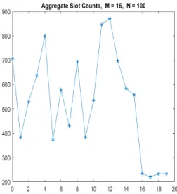
As discussed in Chapter 2, slot synchronization is accomplished via the addition of a certain number of guard slots P, slots in which a pulse is never transmitted, between PPM symbols. By aggregating slot counts over a certain number symbols N, on the order of 2-3 times the PPM order M, the guard slots become apparent and an estimate for the slot offset tau can be calculated using the maximum likelihood estimator

Figure 3-1: Aggregate Slots with an offset of 3.5

Figure 3-2: Aggregate Slots After Shifting

derived here [36]. Tau needs to be calculated M+P times over the given aggregate slot counts for reasons described in [36], but this calculation can be parallelized due to only being dependent on the aggregate slot counts and channel statistics. The tau which maximizes the likelihood function is then taken to be the correct one, doing the likelihood calculation in parallel, and the slot counts (not aggregate slot counts) are shifted over the window of size N according to this tau, depicted in Figure. This occurs codeword size n+N symbols divided by N times in parallel to increase processing throughput, the goal being for the receiver to be able to process one codeword in the time it takes for another codeword to be sent, so as to achieve real-time performance.

3.3.2

MF/FAS Frame Synchronization

The other component of clock recovery is finding the beginning of a frame, which becomes a codeword when the FAS is taken off. The frame synchronization consists of identifying the FAS discussed in Chapter 2, and this is done via calculating the autocorrelation of the FAS across a frame sized chunk of slot counts, with the size of the FAS varies depending on the PPM order as the optimal FAS changes [17]. The autocorrelation consists of convolving the known FAS with the received signal,

which amounts to a bunch of independent multiplications on each slot within the FAS against a window of the received signal of the same size, and then summing the products together to the autocorrelation value. The max value across the frame is where the FAS is located and thus the beginning of the codeword is identified. The autocorrelation calculation can have all of the multiplications done in parallel, while the sum and subsequent max search can be broken into smaller parallel chunks, reducing the complexity by half.

3.3.3

Log-Likelihood Ratios

Now that the received signal has been aligned as best as possible with the transmitted signal, the slot counts (channel observations) need to be converted into log-likelihood ratios (LLRs) for the decoder. An LLR is the log-likelihood a pulse was sent in a given slot for that symbol, over the sum of the log-likelihoods of each the other pulses not containing a slot. The likelihood is derived from the channel statistics as in [29] [32]. The LLRs for the full received signal can be calculated completely in parallel up to the hardware constraints, with the calculation itself also being reduced complexity with individual threads calculate log-likelihoods and then a block summing them all together.

3.4

Demodulation and Decoding

In order to avoid the loss of information associated with hard decision demodulation for a PPM symbol, the design of the Low Density Parity Check code is constructed over the finite field of q, GF(q), where q is equal to the PPM order M. It has been shown that non-binary LDPC (NB-LDPC) codes perform better than binary ones [15] [28], and since PPM is used, PPM symbols can be one to one mapped to elements of GF(q), avoiding the permutation complexities associated with decoding a NB-LDPC, as there is no probability of individual bit error within the field element, only a full symbol error, so there is no need to permute the bit probabilities around within the decoder.

3.4.1

Code Design

Using the code design approach detailed here [28], a non-binary LDPC protograph is selected with the desired BER. The Tanner graph, which is equivalent to the parity check matrix H, is created via a combination of a Progressive Edge Growth (PEG) algorithm [23] and a randomized approach. The PEG ensures a minimum codeword distance and the randomized approach increases the extrinsic information available to the decoder. The parity check matrix is then put in standard form and converted to a generator matrix for encoding [22].

3.4.2

Inference on Tanner Graph

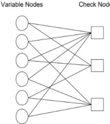
Figure 3-3: Example of a Tanner Graph, variable nodes represent LLRs of transmitted bits, check nodes represent parity constraints dictating the update rule

The decoding makes use of the Tanner graph structure of the LDPC code. Gal-lagher detailed the Belief Propagation algorithm in his 1960 thesis [19], but this was computationally infeasible at the time as most maximum-likelihood approaches were. Tanner also did not write his paper on Tanner graphs until 1981 [40], which offered an efficient data structure for doing the belief propagation decoding.

A Tanner graph turns a parity check matrix into a bipartite graph which by definition has two types of nodes, in the case of Tanner graphs referred to as check and

variable nodes. Check nodes represent the parity constraints ∑︀𝑛

𝑗=0ℎ𝑖𝑗 *𝑐𝑗 = 0, with

ℎ𝑖𝑗 being elements of H and 𝑐𝑗 an elements of the codeword vector C, and variable

nodes to the received bits. Belief propagation operates on the graph as a message passing algorithm, where variable nodes receive messages𝜇𝑐from check nodes, update

their likelihoods𝑦, and send these updated likelihoods to check nodes as messages𝜇𝑣.

Check nodes then calculate their messages based off the parity constraint and send these back to variable nodes for the next update, and this goes on until the variable node likelihoods reach some threshold, or a set number of iterations is reached. The calculations performed at the nodes depend on which decoding algorithm is used, but these fall into two broad categories, Sum-Product (SP) and Min-Sum (MS) [24] [25] [13] [14].

Min-Sum is also referred to as Max-Sum, or Max-Product depending on the sit-uation. It will be referred to only as Min-Sum for the rest of this thesis. Min-Sum works as an approximation of the Sum-Product algorithm, by reducing the complex-ity of the check node operation. A check node calculates the likelihood each of its neighboring variable nodes is a certain element of the GF(q) by finding the likelihood the other neighbors are a combination that would satisfy the parity constraint if the variable node was that certain element. In SP, this calculation is dominated by a large number of distinct products, or sums in the case LLRs are being used, but the observation that these products or sums are dominated by the minimum likelihood in that combination leads to the MS algorithm. This is particularly important for the non-binary case being worked with, as the complexity scales exponentially with both the degree of the check constraint and the order of the finite field used.

3.4.3

Node Calculations and Approximations

Nominally, the variable nodes all have an LLR for each element of GF(q), which is initialized based on the channel observation and subsequently updated as the LLR from the previous iteration plus the sum of messages (Σ𝜇𝑖) from each of its neighbors

(check nodes). The sums scale linearly in complexity with the variable node degree, and the whole step for a given variable node scales linearly with the PPM order, but

the individual sums can be done in parallel.

𝜇𝑣 =𝜇𝑣,𝑝𝑟𝑒𝑣+

∑︁

𝑛𝜖𝜇𝑐

𝜇𝑛

variable node calculation

𝜇𝑐=

∏︁

𝑛𝜖𝜇𝑣

𝜇𝑛

optimal check node calculation

Careful consideration must be made in reducing the complexity of the check node calculation through approximations. The first simplification is to throw out all but the two largest LLRs at each variable node, as is done in the SCPPM case [29] [10]. A dynamic approach could also be taken, where the max LLR is found, and the number of other LLRs kept is based on their value relative to the max. The dynamic approach merits further research, but is not examined in the implementation for this thesis. Using only the two largest LLRs caps the check and variable node calculations from scaling with the PPM order, and constrains the complexity to a similar order of magnitude as the binary case. An important implementation consideration is the overhead of doing arithmetic on a finite field. As the finite field order is equal to the PPM order, only fields of up to 27 _{are used, so a lookup table approach to addition}

and multiplication can be used with minimal impact on memory and complexity. The lookup tables for the different finite fields can be created and stored before processing begins, and so no overhead is associated with this process during the algorithm.

For the check node calculation, the combinations which satisfy the parity con-straint need to be generated based on the two LLRs coming from each of the neigh-bors of the check node so as part of the initialization step for the Tanner graph; this happens at each of the check nodes. The number of combinations that satisfy the parity constraint for a given PPM symbol is equal to 𝑀𝑑𝑐−2_.

With these initialization steps done at their relevant node types, iterative decod-ing now begins with the check node calculations given the channel observation as the initial messages from the variable nodes. The data input to this step comes as

mes-sages from each of the neighbors of the check node, with the mesmes-sages being vectors of LLRs of rank 2.

3.4.4

Parallel Node Implementation

Iterative decoding via belief propagation is traditionally thought of in two steps, the variable node step and check node step, with some of the literature naming an initial step called LLR initialization and a final decision step where decoding terminates and bit decisions are made. In this setup, message passing occurs at the end of each variable and check node step and is not considered a separate part of the algorithm. For a parallel implementation though, it merits its own step in between each variable and check node step with detailed thought given to its data structures and execution, so as to avoid race conditions but also as a means of improving the algorithmic efficiency of the check and variable node steps.

The variable node contains two LLRs, and is updating these with the all of its incoming messages. A variable nodes messages consist of its current belief to all of its neighbors, but minus the most recent message from the respective neighbor its sending a message to, meaning it has to send𝑑𝑣 distinct messages each step. This is

represented as the one global copy of the variable LLR, then a bunch of local messages that are calculated and passed in parallel to the appropriate check nodes. The check node does not have its own LLR to keep track of, instead just needing to act as a vehicle for passing the relevant LLRs combined together through a product to its neighbors so they can update their variable belief. This view breaks the decoder into 4 steps, variable sum, the variable subtraction and send, the check product, and the check send, with the most intensive step being the check product.

Chapter 4

Results

The results detailed in this chapter are all for PPM Order (M) of 16 and codeword length of 3000. The data rate throughput can then be calculated as (3000 symbols * 4 bits/symbol)/(Processing Time). The GPU Occupancy refers to the percent-age of each warp scheduler used, essentially being a measure of how many parallel instructions are used for a given multiprocessor [2].

4.1

Slot Synchronization

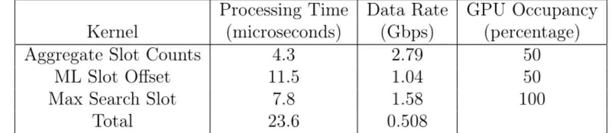
The implementation of slot synchronization can be broken up into three separate kernels performing the aggregation of slot counts, the slot offset and likelihood calcu-lations, and the max likelihood search respectively. This separation is appropriate as they lend themselves to different parallel structure. The receiver is being fed a code-word sized chunk of slot counts, the received signal, and the received signal needs to be aligned with the receiver’s best estimate of the transmitted signal. As described in Chapter 3, the received signal is broken up into windows of size 𝑁 PPM symbols, with an aggregate PPM symbol consisting of 𝑀 +𝑃 aggregate slot counts, where

𝑀 and 𝑃 are the PPM order and ISGT respectively. The aggregate slot counts are generated in the kernel by spawning _𝑁𝑛 blocks, with 𝑛 the length of a codeword in PPM symbols, with𝑀+𝑃 threads, with each block corresponding to an aggregation window and each thread corresponding to an aggregate slot count in that window. A

thread then iterates over the whole window, adding the relevant slot count in the 𝑁

symbols of the window to its aggregate count. The offset and likelihood calculation kernel takes the aggregate counts as inputs, spawning the same number of blocks and threads as the previous kernel, with each thread calculating a slot offset tau and a likelihood sum that this is the slot offset for this aggregation window. The max like-lihood search kernel then spawns N threads and finds the maximum likelike-lihood offset and passes it to the shifting slot count kernel, which corrects the received signal.

The results in this chapter are for the NVIDIA GPU described in Chapter 3. As can be seen in Table 4.1, slot synchronization as implemented does not saturate the GPU even for the maximum codeword length considered. The GPU manages to process a codeword at rates of 100s of Mbps, satisfying the current speed requirements for lasercom.

Table 4.1: Slot Synchronization Performance, M = 16, n = 3000, N = 100 averaged over 30 runs.

Processing Time Data Rate GPU Occupancy Kernel (microseconds) (Gbps) (percentage) Aggregate Slot Counts 4.3 2.79 50

ML Slot Offset 11.5 1.04 50

Max Search Slot 7.8 1.58 100

Total 23.6 0.508

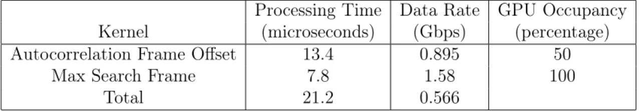
4.2

Frame Synchronization

Frame synchronization works on the individual slot counts as opposed to the aggregate slot counts in slot synchronization. Only two kernels were implemented, one for the autocorrelation and the other using the max search kernel from slot synchronization. The autocorrelation kernel spawns𝑛threads, broken up into blocks so as to maximize warp efficiency. Each thread runs an autocorrelation loop over 𝑁 symbols, where 𝑁

is the length of the FAS, requiring 𝑁 multiplications and additions, ignoring the non-pulse slots as the frame synchronization occurs after the slot synchronization, assuming the slot clock is accurately aligned as to reduce complexity by ignoring

non-pulse slots. The max search is the same as in slot synchronization.

Frame synchronization also happens at similar speeds to slot synchronization, as can be seen in Table 4.2, and the complexity reduction used does not increase error probability since slot sync is done optimally beforehand [36].

Table 4.2: Frame Synchronization Performance, M =16, n= 3000, N=17 averaged over 30 runs

Processing Time Data Rate GPU Occupancy Kernel (microseconds) (Gbps) (percentage) Autocorrelation Frame Offset 13.4 0.895 50

Max Search Frame 7.8 1.58 100

Total 21.2 0.566

4.3

LLR Generation

LLR generation calculates an LLR for each slot of the received signal, removing the guard slots in the process. It therefore needs to do 𝑛*𝑀 LLR calculations, where 𝑛

is the codeword length in PPM symbols, and𝑀 is the PPM order. For the LLR, the log-likelihood a slot is a signal pulse is calculated, and then divided by the summed log-likelihoods the other slots in this PPM symbol are not a signal pulse. To do this effectively in parallel, 𝑛*𝑀 threads are launched, with each thread responsible for one slot and calculating the log-likelihood of the slot being a signal pulse and the log-likelihood of the slot not being a signal pulse. The threads are then synced, and each thread sums the log-likelihoods the other slots in the PPM symbol are not signal pulses and divides the log-likelihood the slot is a signal pulse by this sum to get the LLR.

The kernel block size can be made into a multiple of 32 (the warp size) without excess computational overhead for indexing, as is the case in frame sync and slot sync where the guard times make it challenging to concisely index PPM symbols in multiples of 32. This means the LLR generation reaches 100 percent GPU occupancy as seen in 4.3. It also keeps the computational burden at similar throughputs as frame and slot sync.

Table 4.3: LLR Generation Performance, M =16, n = 3000, averaged over 30 runs Processing Time Data Rate GPU Occupancy

Kernel (microseconds) (Gbps) (percentage) LLR Generation 16.1 0.745 100

4.4

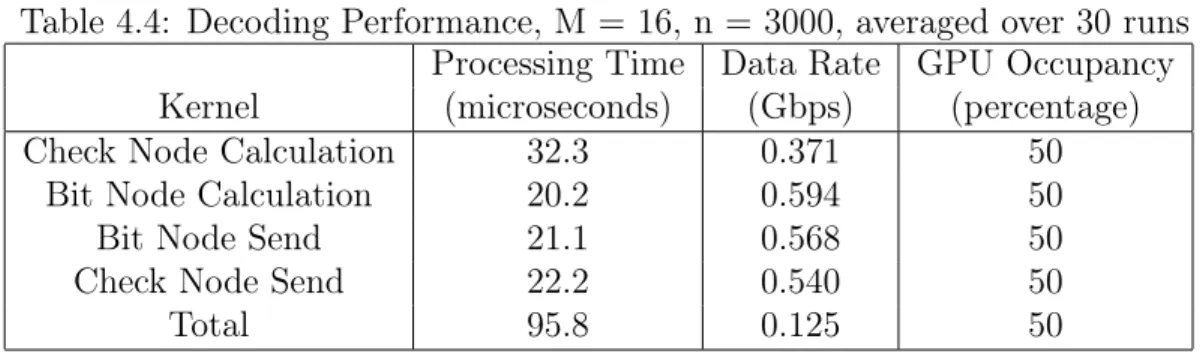
Decoding

Decoding breaks down into four kernels, with the results shown in Table 4.4. The check node calculation kernel most intensive as expected

Table 4.4: Decoding Performance, M =16, n = 3000, averaged over 30 runs Processing Time Data Rate GPU Occupancy Kernel (microseconds) (Gbps) (percentage) Check Node Calculation 32.3 0.371 50

Bit Node Calculation 20.2 0.594 50

Bit Node Send 21.1 0.568 50

Check Node Send 22.2 0.540 50

Chapter 5

Summary

5.1

Conclusions

It has been shown that using a typical GPU found in a modern laptop, the signal processing chain for lasercom receivers can be performed to support current lasercom data rate requirements for small satellites while reducing the complexity of electronics and programming needed. In order to do this, only the forward error correction scheme had to be changed from current methods used in lasercom systems. LDPC-PPM, the FEC scheme used in this thesis, is able to arbitrarily approach capacity in the same way SCPPM is, but lends itself to a higher degree of parallel decoding, meaning theoretical performance is not sacrificed to achieve lower complexity parallel decoding as seen in Section 3.4. It also means it will be able to scale more effectively than SCPPM as GPUs add more parallel processors, which will be necessary in future lasercom systems trying to scale to hundreds of Gbps.

5.2

Future Work

This thesis only analyzes shorter block length LDPC codes. There should be no problem scaling the decoding implementation to longer block lengths, but further investigation is required to verify the performance can compete with SCPPM in the low photon regime of deep space links. Additionally, LDPC codes have been shown to

work well in both high rate and low rate scenarios, meaning they can be used for both small satellite LEO missions as well as deep space missions. To fully take advantage of LDPC codes, variable rate coding architectures could be used, offering increased flexibility to lasercom systems. Further improvements to the decoding algorithm could be made as well, with more analysis on how many LLRs need to be kept, and how to best approximate the check node calculations.

GPUs have only recently become popular as general purpose computing platforms, and as a result, their use in embedded systems for communications has been minimal. Developing and testing flight computers which include NVIDIA SoCs with GPUs on them is another area for future work, which will require identifying failure modes of GPUs in the space environment and doing radiation testing to find their limits. There are additional benefits outside of lasercom for implementing GPUs as flight computers, as GPUs can enable small satellites to perform a wider variety of tasks in image processing [4] and possibly allow them to employ machine learning algorithms on orbit.

Bibliography

[1] JESD204B Overview Texas Instruments High Speed Data Converter Training. Technical report.

[2] NVIDIA Tesla P100.

[3] Near Field Infrared Experiment ( NFIRE ) missile phenomenology data collection satellite. Technical report, 2006.

[4] Caleb Adams and David Cotten. A Near Real Time Space Based Computer Vision System for Accurate Terrain Mapping. In32nd Annual AIAA/USU Con-ference on Small Satellites, 2018.

[5] Shuichi Asano, Tsutomu Maruyama, and Yoshiki Yamaguchi. Performance Comaprison of FPGA, GPU and CPU in image processing. In International Conference on Field Progammable Logic and Applications, pages 126–131, 2009. [6] Claude Berrou and Alain Glavieux. Near Optimum Error Correcting Coding And Decoding: Turbo-Codes. IEEE Transactions on Communications, 44(October), 1996.

[7] Abhijit Biswas, Joseph M Kovalik, Malcolm W Wright, William T Roberts, Michael K Cheng, Abhijit Biswas, Joseph M Kovalik, Malcolm W Wright, William T Roberts, Michael K Cheng, Kevin J Quirk, Meera Srinivasan, Matthew D Shaw, Abhijit Biswas, Joseph M Kovalik, Malcolm W Wright, William T Roberts, Michael K Cheng, Kevin J Quirk, Meera Srinivasan, Matthew D Shaw, and Kevin M Birnbaum. LLCD operations usign the Optical Communications Telescope Laboratory (OCTL). In Free-Space Laser Commu-nication and Atmospheric Propagation XXVI, 2014.

[8] Don M Boroson, Bryan S Robinson, Daniel V Murphy, Dennis A Burianek, Farzana Khatri, Don M Boroson, Bryan S Robinson, Daniel V Murphy, Den-nis A Burianek, Farzana Khatri, Joseph M Kovalik, Zoran Sodnik, and Donald M Cornwell. Overview and results of the Lunar Laser Communication Demonstra-tion. In Free-Space Laser Communication and Atmospheric Propagation XXVI, 2014.

[9] David O. Caplan. Laser communication transmitter and receiver design. In

Journal of Optical and Fiber Communications Reports, volume 4, pages 225– 362. 2007.

[10] M K Cheng, M A Nakashima, J Hamkins, B E Moision, and M Barsoum. A Field-Programmable Gate Array Implementation of the Serially Concatenated Pulse-Position. The Interplanetary Network Progress Report, 42(114), 2005. [11] Emily Clements, Raichelle Aniceto, Derek Barnes, David Caplan, James Clark,

Inigo del Portillo, Christian Haughwot, Maxim Khatsenko, Ryan Kingsbury, My-ron Lee, Rachel Morgan, Jonathan Twichell, Kathleen Riesing, Hyosang Yoon, Caleb Ziegler, and Kerri Cahoy. Nanosatellite optical downlink experiment: de-sign, simulation, and prototyping. SPIE Optical Engineering, 55(11):111610–1 – 11610–18, 2016.

[12] NVIDIA Corporation. NVIDIA CUDA C Programming Guide, 2018.

[13] David Declercq and Marc Fossorier. Extended MinSum Algorithm for Decoding LDPC Codes over GF ( q ). In IEEE International Symposium on Information Theory, 2005.

[14] David Declercq and Marc Fossorier. Decoding Algorithms for Nonbinary LDPC Codes over GF(q). IEEE Transactions on Communications, 55(4), 2007.

[15] Lara Dolecek, Dariush Divsalar, Yizeng Sun, and Behzad Amiri. Non-Binary Protograph-Based LDPC Codes : Enumerators, Analysis, and Designs. IEEE Transactions on Information Theory, 60(7):3913–3941, 2014.

[16] William H. Farr, Jeffrey A. Stern, and Matthew D. Shaw. Superconducting nanowire arrays for multi-meter free-space optical communications receivers. In

Free-Space Laser Communication and Atmospheric Propagation XXIV, number February 2012, 2012.

[17] R. Gagliardi, J. Robbins, and H. Taylor. Acquisition Sequences in PPM Com-munications. IEEE Transactions on Information Theory, 33(5):738–744, 1987. [18] Robert M. Gagliardi and Sherman Karp. Optical Communications. Wiley, 1995. [19] Robert G. Gallagher. Low-Density Parity-Check Codes. M.I.T. Press, 1963. [20] Hamid Hemmati. Deep Space Optical Communications. John Wiley and Sons,

Inc., Boca Raton, FL, 2006.

[21] Hamid Hemmati. Near-Earth Laser Communications. CRC Press, Boca Raton, FL, 2009.

[22] Raymond Hill. A First Course in Coding Theory. Clarendon Press, 1986. [23] Xiao-yu Hu, Evangelos Eleftheriou, and Dieter M Arnold. Regular and Irregular

Progressive Edge-Growth Tanner Graphs. IEEE Transactions on Information Theory, 51(1):386–398, 2005.

[24] Qin Huang, Senior Member, Liyuan Song, and Zulin Wang. Set Message-Passing Decoding Algorithms for Regular Non-Binary LDPC Codes. IEEE Transactions on Communications, 65(12):5110–5122, 2017.

[25] Selcuk Keskin and Taskin Kocak. GPU-Based Gigabit LDPC Decoder. IEEE Communications Letters, 21(8):1703–1706, 2017.

[26] Ryan Kingsbury.Optical Communications for Small Satellites. PhD thesis, 2015. [27] David J. Mackay. Inference, Information, and Learning. Cambridge University

Press, 2003.

[28] Balázs Matuz, Enrico Paolini, Flavio Zabini, Gianluigi Liva, and Senior Member. Non-Binary LDPC Code Design for the Poisson PPM Channel. IEEE Transac-tions on CommunicaTransac-tions, 65(11):4600–4611, 2017.

[29] B Moisson and J Hamkins. Coded Modulation for the Deep-Space Optical Chan-nel : Serially Concatenated Pulse-Position Modulation. The Interplanetary Net-work Progress Report, 42(161), 2005.

[30] Daniel V Murphy, Jan E Kansky, Matthew E Grein, Robert T Schulein, Matthew M Willis, Daniel V Murphy, Jan E Kansky, Matthew E Grein, Robert T Schulein, Matthew M Willis, and Robert E Lafon. LLCD operations using the Lunar Lasercom Ground Terminal. In Free-Space Laser Communication and Atmospheric Propagation XXVI, number March 2014, 2014.

[31] Ryan Nugent and Alexander Chin. The CubeSat : The Picosatellite Standard for Research and Education. In AIAA SPACE 2008 Conference & Exposition, number September 2008, 2008.

[32] Kevin J. Quirk and Meera Srinivasan. Optical PPM demodulation from slot-sampled photon counting detectors. In MILCOM 2013 - IEEE Military Com-munications Conference, pages 1634–1638, 2013.

[33] Thomas J Richardson, M Amin Shokrollahi, and Rüdiger L Urbanke. Design of Capacity-Approaching Irregular Low-Density Parity-Check Codes. IEEE Trans-actions on Information Theory, 47(2):619–637, 2001.

[34] Tom Richardson and Rüdiger Urbanke. Modern Coding Theory. Cambridge University Press, 2008.

[35] Kathleen Michelle Riesing. Portable Optical Ground Stations for Satellite Com-munication. PhD thesis, 2018.

[36] Ryan Rogalin and Meera Srinivasan. Maximum likelihood synchronization for pulse position modulation with inter-symbol guard times. In 2016 IEEE Global Communications Conference, (GLOBECOM), 2016.

[37] T S Rose, D W Rowen, S Lalumondiere, R Linares, A Faler, J Wicker, C M Coff-man, G A Maul, D H Chien, A Utter, and R P Welle. Optical Communications Downlink from a 1.5U CubeSat: OCSD Program. In AIAA/USU Conference on Small Satellites, 2018.

[38] Marek Rupniewski and Gustaw Mazurek. A Real-Time Embedded Hetero-geneous GPU / FPGA Parallel System for Radar Signal Processing. In

2016 Intl IEEE Conferences on Ubiquitous Intelligence & Computing, Ad-vanced and Trusted Computing, Scalable Computing and Communications, Cloud and Big Data Computing, Internet of People, and Smart World Congress (UIC/ATC/ScalCom/CBDCom/IoP/SmartWorld), pages 1189–1197, 2016. [39] Claude Shannon. A Mathematical Theory of Communication. The Bell System

Technical Journal, 27:379–423, 1948.

[40] R Michael Tanner. A Recursive Approach to Low Complexity Codes. IEEE Transactions on Information Theory, 27(5):533–547, 1981.

[41] Jekan Thangavelautham and Pranay Reddy Gankidi. FPGA Architecture for Deep Learning and its application to Planetary Robotics Pranay Reddy Gankidi Space and Terrestrial Robotic Exploration (SpaceTREx) Lab. InIEEE Aerospace Conference, number March, 2017.

[42] Robert Tyson. Principles of Adaptive Optics. Academic Press, 2012.

[43] M M Willis, A J Kerman, M E Grein, J Kansky, B R Romkey, E A Dauler, D Rosenberg, B S Robinson, D V Murphy, and D M Boroson. Performance of a Multimode Photon-Counting Optical Receiver for the NASA Lunar Laser Communications Demonstration. In International Conference on Space Optical Systems and Applications, volume 12, pages 3–5, 2012.

[44] M. M. Willis, B. S. Robinson, M. L. Stevens, B. R. Romkey, J. A. Matthews, J. A. Greco, M. E. Grein, E. A. Dauler, A. J. Kerman, D. Rosenberg, D. V. Murphy, and D. M. Boroson. Downlink synchronization for the lunar laser communications demonstration. In 2011 International Conference on Space Optical Systems and Applications, ICSOS’11, pages 83–87, 2011.

[45] Hyosang Yoon. Pointing System Performance Analysis for Optical Inter-satellite Communication on CubeSats. PhD thesis, 2017.

[46] Caleb Kevin Ziegler. A Jam-Resistant CubeSat Communications Architecture. PhD thesis, 2017.