Robust Value at Risk Prediction

(1)

Robust Value at Risk Prediction

LORIANOMANCINI

Sw iss Finance Institute and Ecole Polytechnique F´ed´erale de Lausanne

FABIOTROJANI

Sw iss Finance Institute and U niversity ofLugano

ABSTRACT

This paper proposes a robust semiparametric bootstrap method to estimate predictive distributions of GARCH-type models. The method is based on a robust estimation of parametric GARCH models and a robustified resampling scheme for GARCH residuals that controls bootstrap instability due to outlying observations. A Monte Carlo simulation shows that our robust method provides more accurate Value at Risk (VaR) forecasts than classical methods, often by a large extent, especially for several days ahead horizons and/or in presence of outlying observations. An empirical application confirms the simula-tion results. The robust procedure outperforms in backtesting several other VaR prediction methods, such as RiskMetrics, CAViaR, histori-cal simulation, and classihistori-cal filtered historihistori-cal simulation methods. We show empirically that robust estimation reduces tail estimation risk, providing more accurate and more stable VaR prediction intervals over

time. (JEL:C14, C15, C23, C59)

KEYWORDS: backtesting, breakdown point,M-estimator, extreme value

theory

Large portfolios of traded assets held by many financial firms have made the mea-surement of market risk, that is, the risk of losses on the trading book due to ad-verse market movements, a primary concern for regulators, and risk managers.

For helpful comments we thank Eric Renault (the editor), the associate editor, two anonymous referees, Claudio Ortelli, Franco Peracchi, and Claudia Ravanelli. We gratefully acknowledge the financial support of the Swiss National Science Foundation (NCCR-FinRisk, Grants num-bers 101312-103781/1 and 100012-105745/1). Address correspondence to Loriano Mancini, Swiss Finance Institute at EPFL, Quartier UNIL-Dorigny, CH-1015 Lausanne, Switzerland, or e-mail: [email protected].

doi: 10.1093/jjfinec/nbq035 c

at UniversitÃ© & EPFL Lausanne on May 17, 2011

jfec.oxfordjournals.org

(2)

TheBasel Committee(1996) requires that financial firms hold a certain amount of capital against market risk. This capital is called Value at Risk (VaR) and must be sufficient to cover losses on the trading book over a 10-day holding period 99% of the times. In practice, VaR is computed for several holding periods and confidence levels, such as 95% confidence level and horizon of 1 day.

From a statistical viewpoint, VaR is the quantile of the profit and loss (P&L) distribution of a portfolio over a certain holding period. Hence, a key issue in implementing VaR and related risk measures is to obtain accurate estimates for the tails of conditional P&L distributions.

Semiparametric methods, commonly called filtered historical simulation (FHS) methods, have been found to provide rather accurate estimates of P&L distributions; see, for example,Pritsker (1997), Hull and White(1998),Diebold, Schuermann, and Stroughair (1998), Barone-Adesi, Giannopoulos, and Vosper (1999),McNeil and Frey(2000),Pritsker(2001), andKuester, Mittnik, and Paolella (2006). In FHS methods, parametric GARCH-type models are typically fitted to historical returns using pseudo maximum likelihood (PML). Then GARCH resid-uals are resampled using bootstrap methods. The FHS methods allow for time-varying conditional moments of returns (via GARCH-type models) and non-parametric structures in conditional distribution of returns (because innovation distributions are estimated nonparametrically). The last feature is crucial in appli-cations and avoids too simplistic assumptions on return conditional distributions, such as normality; see, for example, JP Morgan’sRiskMetrics(1995).

In this paper, we propose a general robust semiparametric bootstrap method to estimate predictive distributions of asset returns in GARCH-type volatility mod-els. The method allows for general parametric specifications of time-varying conditional mean and volatility of asset returns. As an application, we use the proposed robust method to predict VaR over different forecasting horizons. Our approach achieves robustness in two steps. In the first step, we estimate a paramet-ric GARCH-type model using the optimal bounded influence estimator inMancini, Ronchetti, and Trojani(2005). In the second step, we fit generalized Pareto distribu-tion (GPD) using the robust estimator inDupuis(1999) andJu´arez and Schucany (2004) to the tails of GARCH residuals distribution and we resample from this dis-tribution. In order to ensure robustness of the whole procedure, both robustification steps are necessary.

PML estimators with Gaussian pseudo densities are often used to fit GARCH-type models and they feature a number of convenient theoretical properties. For instance, they achieve maximal efficiency (being maximum likelihood) when turns are indeed conditionally Gaussian. Moreover, even under non-Gaussian re-turns, they imply consistent estimation of the parameters in the conditional mean and variance functions, provided the latter are correctly specified. Finally, in some cases, Gaussian PML estimators coincide with weighted nonlinear least squares estimators and can achieve the semiparametric efficiency bound for estimating a correctly specified conditional moment function.

(3)

In the more general situation of (i) potentially misspecified conditional mean and variance functions and (ii) non Gaussian returns, these convenient properties of PML can break down. In this case, PML implicitly estimates a pseudo true value for the conditional GARCH dynamics, which minimizes the Kullback–Leibler dis-crepancy between the unknown conditional density of returns and a parametric family of Gaussian pseudo likelihoods. A major issue is that even if the relevant degree of misspecification might be small, in the sense that the true conditional moments of the data-generating process might be only slightly different from those specified under the parametric GARCH assumption, there is no guarantee that the conditional moment function implied by the theoretical pseudo true value will again be only slightly different from the true one; see, for example, Sakata and White (1998) and Mancini, Ronchetti, and Trojani (2005) for some concrete evi-dence on this point. Similarly, under such circumstances, there is no guarantee that PML can produce estimates of the pseudo true conditional mean and variance functions that are comparably efficient as in the case of a correct specification of the latter. These features of Gaussian PML are strongly related to the functional struc-ture of these estimators, which implies excess sensitivity of pseudo true values and PML asymptotic covariance matrices with respect to the underlying data distribu-tion. Such a sensitivity or nonrobustness of these estimators can be problematic because even a moderate misspecification of the assumed parametric model can lead to either strongly biased or inefficient results, for example, in terms of the implied mean square error (MSE) for the estimated conditional moments.

In this paper, we apply a class of robustM-estimators for GARCH-type mod-els proposed in Mancini, Ronchetti, and Trojani(2005). These estimators ensure smoothness of the implied pseudo true value with respect to the underlying data distribution using a set of robustified moment conditions defined by a bounded estimating function. The robust estimating function is obtained from the Gaussian PML score function by a downweighting procedure. This procedure bounds the potential damaging effects of data points generating a large sensitivity of theo-retical PML pseudo true values with respect to the underlying data distribution. Our estimators provide robust, that is, smooth, estimation results in an abstract nonparametric neighborhood of a fixed reference model, which we take to be a GARCH-type model with Gaussian errors. In general, a trade off between robust-ness (with respect to model misspecification) and efficiency (under a correct model specification) emerges when choosing between robust and PML estimators, and the researcher has to decide on this trade off. It is an empirical question whether the quantitative effects of a small misspecification of GARCH-type models, for example, in the form of an incorrect variance dynamics, can lean the trade off in favor of using robust methods in the estimation of GARCH-models for pre-dicting VaR.Sakata and White(1998) andMancini, Ronchetti, and Trojani(2005), among others, show that such a favorable trade off exists when estimating condi-tional variance dynamics already under a moderate model misspecification. In our Monte Carlo simulations, we find that robust GARCH estimators combined with a robust extreme value estimator for the conditional tails of returns produce lower

(4)

MSEs in forecasting the true VaR already under very small misspecifications of the assumed parametric model.

The issue of the impact of a model misspecification on the statistical properties of an estimator is even more pronounced when fitting innovation tail distributions, as required for VaR predictions. For instance, generalized Pareto dis-tribution (GPD) is typically used in extreme value theory to model tail distribu-tions of returns above a given threshold. Theoretically, the GPD is an asymptotic approximation of the tail, which improves in the limit as the threshold goes to infinity (or to the end point of the distribution). In practice, however, the thresh-old is fixed and the error implied by the GPD approximation for the true tail dis-tribution can have nontrivial consequences for the properties of PML estimators based on a GPD pseudo density. This is so because the GPD PML score leads to an unbounded estimating function that implies nonsmooth pseudo true values with respect to variations of the underlying data distribution. In this context, the robust GPD estimator in our approach is a natural estimator because it is based on a bounded estimating function that explicitly downweights the damaging effects of a potential misspecification of the tail specified by the GPD, thus providing more accurate estimators when such deviations are indeed present in the data. We con-firm this intuition in several Monte Carlo simulations, showing that robust GPD estimator provides more accurate quantile estimates (e.g., in terms of a lower MSE) under a number of realistic specifications of the tail. These estimates are also much less sensitive to the choice of threshold levels than classical methods. The latter is a further desirable property of the robust estimator because in applications the selection of the threshold level is a difficult task.

Another important issue is the nonrobustness of several resampling proce-dures used to compute VaR estimates at several days ahead horizons. It has been recognized that a few large observations are sufficient to cause the break down of quantile estimates based on nonparametric residual bootstrap; see, among oth-ers,Singh(1998), Gagliardini, Trojani, and Urga(2005), Davidson and Flachaire (2007), andCamponovo, Scaillet, and Trojani(2009,2010). We find that standard nonparametric bootstrap procedures for VaR computation have a very low break-down point (BP), meaning that VaR forecasts can be heavily affected already by a few large observations, especially when longer forecast horizons of, for example, 10 days are considered. Using the robust GPD estimator in our approach, we are also able to develop a resampling procedure for VaR forecasting that controls for the instability generated by outlying observations in estimated GARCH residual distributions; see alsoCowell and Victoria-Feser(1996).

We perform an extensive Monte Carlo simulation and show that our robust method provides more accurate VaR predictions than classical methods under con-ditionally non-Gaussian data, in particular, for several days ahead horizons. When the GARCH model used to predict VaR is not exactly the same as the true data-generating process, robust VaR predictions have mean square prediction errors several times smaller than those of classical procedures. In nearly all Monte Carlo experiments, our robust procedure has the lowest mean square prediction errors,

(5)

often by a large extent. In contrast to classical methods, our procedure never fails validation tests at 10% confidence level.

The simulation evidence is confirmed by the real data application. We backtest VaR prediction methods using about 20 years of S&P 500, Dollar-Yen, Microsoft, and Boeing historical returns. We compare our method to several alternative VaR prediction procedures, such as (i) historical simulation, (ii) RiskMetrics, (iii) semi-parametric GARCH model of Engle and Gonzalez-Rivera (1991), (iv) CAViaR model ofEngle and Manganelli(2004), and for 10-day ahead VaR predictions, (v) GARCH model applied directly to 10-day asset returns. Only our robust method passes all validation tests at 10% confidence level. Moreover, we find that the re-duction in tail estimation risk of our robust procedure provides more accurate and more stable VaR prediction intervals over time. For instance, in the case of S&P 500 and Boeing, robust VaR prediction intervals are nearly 20% narrower and 50% less volatile than classical ones. Given the higher accuracy of robust VaR predictions documented in violation tests, the stability over time of robust VaR profiles is a feature that allows financial firms to adapt properly risky positions to VaR limits more smoothly and thus more efficiently.

Section 1introduces classical and robust semiparametric bootstrap methods for VaR predictions. Section2presents Monte Carlo evidence on VaR predictions under different forms of conditional nonnormal returns. Section3presents the real data application and backtesting for four financial time series. Section4concludes.

1 SETTING

1.1 Return Dynamics and Measures of Market Risk

LetY := {Yt}t∈Zbe a strictly stationary time series process on probability space

(R∞,_F,P_∗), modeling the daily rate of return on a financial asset with pricePtat time t, that is, Yt := Pt/Pt−1−1. We assume that distribution P_∗ can be

“approximated” by a parametric reference model P_θ₀ in the parametric family

P := {P_θ,θ ∈ Θ ⊆ Rp}. Even ifP_∗ might not be a member ofP, so that the parametric family is misspecified, we assume that P_∗ belongs to a

nonparamet-ric neighborhood ofP_θ₀, denoted byU(P_θ₀). The neighborhood is assumed to be small, in the sense that the distribution distance between P_∗andP_θ₀ is assumed

to be moderate.

Remark 1.1. NeighborhoodU(P_θ₀)can be defined using different metrics between

distributions, and it represents a proximity of similar models used to provide an approximate statistical description ofP_∗. Robust estimators are designed to

pro-vide a smooth statistical behavior over neighborhoodU(P_θ₀)in order to make the estimator’s properties not excessively dependent on which specific direction of misspecification of P_θ₀ might indeed be present in the data. In applications, the

specific size of neighborhoodU(P_θ₀)is in most cases only implicitly fixed by the

(6)

degree of robustness imposed on the estimator used. Intuitively, the more robust an estimator the broader the implicit neighborhood of potential model misspeci-fications that are considered as possible relevant data-generating processes in the robust approach.

UnderP_θ₀, we assume that process_Ysatisfies the dynamic model

Yt=μt(θ0) +σt(θ0)Zt, (1) whereμt(θ0)andσt2(θ0)parameterize the conditional mean and conditional vari-ance ofYt, given informationFt−1up to timet−1. UnderPθ0, innovationsZare a strong white noise, that is,Zt∼IIN(0, 1). GivenY₁m:={Y1, . . . ,Ym}, denote byPm_∗

(Pm_θ

0) them-dimensional marginal distribution ofY m

1 underP∗(Pθ0).Ft,t+h is the conditional distribution function ofhdays returnsYt,t+h:=Pt+h/Pt−1 underP_∗,

given informationFt. For 0 < α < 1 and horizon hdays, let yα

t,t+h denote the α-quantile ofF_t_,_t+h, that is,yα

t,t+h := inf{y∈R: Ft,t+h(y)>α}. For an asset with market pricePt, the VaR at timet, confidence levelα, and horizonhdays, VaRαt,t+h, is defined by1

α=P_∗(Pt+h−Pt<−VaRαt,t+h|Ft). (2) Hence,−VaRα

t,t+h = Ptyα_t_,_t+his theα-quantile of the conditional P&L distribution underP_∗over the next hdays, givenFt.2 Another measure of market risk is the expected shortfall (ES,Artzner et al. 1999),Sα

t,t+h := E∗[Yt,t+h|Yt,t+h < yαt,t+h,Ft], whereE∗[∙]denotes expectation with respect toP∗. For horizonh=1 day,

yα

t,t+1=μt+1(θ0) +σt+1(θ0)zα, Sαt,t+1=μt+1(θ0) +σt+1(θ0)E∗[Z|Z<zα], wherezαis theα-quantile of the distribution ofZ. Estimation of VaR or ES can be obtained by estimating model (1) and tail distribution of residuals Z. For longer horizonsh>2, estimating model (1) is only the starting point to compute market risk measures. Joint conditional distributions of{Zt+1, . . . ,Zt+h},{μt+1, . . . ,μt+h}, and{σt+1, . . . ,σt+h}have to be estimated, a task that is considerably more difficult. FHS methods estimate Ft,t+h using semiparametric bootstrap of model (1) over horizon[t,t+h]. Our goal is to develop robust semiparametric bootstrap methods for estimatingFt,t+h.

1.2 Estimation of GARCH-type Models

The parameters of model (1) are usually estimated by PML; see White (1982), Gouri´eroux, Monfort, and Trognon(1984), andBollerslev and Wooldridge(1992).

1_{For brevity, Equation (2) assumes a continuous P&L distribution.}

2_{See, for example,}_{Duffie and Pan}_{(1997) and}_{Gouri´eroux, Laurent, and Scaillet}_{(2000) for a general} dis-cussion on conditional VaR, andA¨ıt-Sahalia and Lo(2000) for an economic interpretation of VaR.

(7)

The functional pseudo maximum likelihood estimator (PMLE)a(∙)is defined by

E∗[s(Y1m;a(Pm∗))] =0, where the Gaussian score function

s(Y1m;θ):= _σ_m21₍_θ₎ ∂μm(θ) ∂θ εm(θ) + 1 2σ_m2(θ) ∂σ_m2(θ) ∂θ ε2_m(θ) σ_m2(θ)−1 (3)

andεm(θ):= σm(θ)Zm. PMLE has a number of convenient and useful properties. First, when true distribution, P_∗, coincides withP_θ₀, PMLE is indeed the

Maxi-mum Likelihood estimator. Second, if the conditional mean and variance functions μm(θ0)andσm2(θ0)are correctly specified, they are consistently estimated even un-der non-Gaussianity of the errors distribution. However, an important issue is that even when the degree of misspecification might be small, for example, with true conditional moments that might be only slightly different from those under the parametric model, there is no guarantee that the pseudo true conditional moments will remain only slightly different from the true ones. This feature of Gaussian PML is determined by the functional structure of these estimators, which implies excess sensitivity of pseudo true values and PML asymptotic covariance matrices with respect to the underlying data distribution. Such a sensitivity or nonrobust-ness of these estimators is due to the fact that the estimating function of Gaussian PMLE is unbounded.

In this paper, we apply a class of robustM-estimators for GARCH-type mod-els proposed in Mancini, Ronchetti, and Trojani(2005). These estimators ensure smoothness of the implied pseudo true value with respect to the underlying data distribution using a set of robustified moment conditions implied by a bounded estimating function. The robust estimating function is obtained from the Gaussian PML score function by a downweighting procedure that bounds the po-tential damaging effects of data points generating a too large sensitivity of Gaussian PML pseudo true values.

Mancini, Ronchetti, and Trojani(2005) robust estimator is efficient and com-putationally feasible for highly nonlinear models and compares favorably with other robust estimators, such as robust Generalized Method of Moments estima-tors (Ronchetti and Trojani 2001) or robust Efficient Method of Moments estimators (Ortelli and Trojani 2005) for time series. It is defined as follows. Let

ψc(s(Y1m;θ)):=A(θ)(s(Y1m;θ)−τ(Y1m−1;θ))w(Y1m;θ), (4) wheres(Y₁m;θ)is the PML score function defined in Equation (3), and

w(Y1m;θ):=min(1,ckA(θ)(s(Y1m;θ)−τ(Y1m−1;θ))k−1). The robust functionalM-estimatora(∙)ofθis defined by

E∗[ψc(s(Y1m;a(Pm∗)))] =0, (5)

(8)

where nonsingular matrixA(θ)∈Rp×Rp andFm−1-measurable random vector

τ(Y₁m−1;θ)∈Rpare determined by the implicit equations

Eθ0[ψc(s(Y1m;θ0))ψc(s(Y1m;θ0))>] =I, (6)

Eθ0[ψc(s(Y1m;θ0))|Fm−1] =0. (7) The estimating functionψc is a truncated version of PML score function (3) be-cause by constructionkψc(s(Y1m;θ))k 6 c. The constantccontrols for the degree of robustness. Whenc = ∞, the robust estimatora in Equation (5) is indeed the PMLE. Section1.5discusses how to selectc.3

To obtain VaR predictions, conditional mean and conditional volatility in model (1) have to be specified; see, for example, Ghysels, Harvey, and Renault (1996). Several GARCH-type models have been proposed in the financial literature. Our robust method can accommodate general specifications forμt(θ0)andσt(θ0) that imply different estimating functions but do not change the overall procedure. In our simulations and empirical applications, we adopt a fairly flexible model, namely an autoregressive AR(1) model for the conditional meanμt(θ0)and an asymmetric GARCH(1,1) model for the conditional varianceσ_t2(θ0)(Glosten, Jagannathan, and Runkle 1993),

μt(θ0) =ρ0+ρ1Yt−1, (8)

σ_t2(θ0) =α0+α1ε2t−1(θ0) +α2σt2−1(θ0) +α3ε2t−1(θ0)It−1(θ0), (9) whereα0,α1,α2 >0,|ρ1|<1,α1+α2+α3/2<1,It−1(θ0) =1 whenεt−1(θ0)<0 and 0 otherwise. The AR(1) model for μt captures potential autocorrelations in daily returns, for instance, due to nonsynchronous transactions in different index components. The parameterα3 > 0 accounts for the leverage effect,4 that

3_{Formally, optimality results in}_{Mancini, Ronchetti, and Trojani}_{(2005) hold for ARCH- but not} GARCH-type models. As inSakata and White(1998), however, we can expect that our robust estimator performs well also under GARCH models with sufficient memory decay. To investigate this point, in the esti-mating function (4), we approximate the GARCH volatility by an ARCH model. For example in the GARCH(1,1) model, σ2_t(θ) =α0+α1ε2_t₋1(θ) +α2σt2−1(θ) = +∞ ∑ j=0 αj₂(α0+α1ε2_t₋1−j(θ)) =l− 1 ∑ j=0 α₂j(α0+α1ε2_t₋1−j(θ)) +αl2σt2−l(θ) =:σ2t(θ)trunc+αl2σt2−l(θ)≈σt2(θ)trunc. For sufficiently large lagl,αl2σt2−l(θ)≈0, and the bias of the robust estimatoratruncbased onσt2(θ)trunc is expected to be negligible. Monte Carlo simulation in Section2.1studies this issue.

4_{The terminology leverage effect was introduced by}_Black_{(1976) who suggested that a large negative} return increases the financial and operating leverage and rises equity return volatility; see alsoChristie (1982).Campbell and Hentschel(1992) suggested an alternative explanation based on the market risk premium and volatility feedback effects; see alsoBekaert and Wu(2000). Following common practice, we shall use the terminology leverage effect when referring to the asymmetric reaction of volatility to positive and negative return innovations.

(9)

is, negative shocks (εt−1(θ0)<0) raise future volatility more than positive shocks (εt−1(θ0)> 0) of the same absolute magnitude. Compared to symmetric GARCH models (α3 = 0), asymmetric GARCH models are better able to fit volatility dynamics of equity and index returns; see, for example,Engle and Ng(1993) and Rosenberg and Engle (2002). To our knowledge, robust estimators of asymmet-ric GARCH models have not yet been applied in the statistics and econometasymmet-rics literature.

1.3 Bootstrap Methods of GARCH-type Processes

We study bootstrap methods for GARCH-type processes consisting of two steps. In the first step, we fit model (8)–(9) to historical returns,y1, . . . ,yT, using either PML or optimal robust estimators, obtaining parameter estimates ˆθ. In the second step, to estimateFT,T+h, we apply various bootstrap procedures to estimated scaled residuals, ˆ zt= yt−μt( ˆ θ) σt(θˆ) , t=1, . . . ,T.

We denote byPTthe empirical distribution of estimated scaled residuals ˆz1, . . . , ˆzT.

1.3.1 Nonparametric residual bootstrap and VaR estimation. Nonpara-metric residual bootstrap relies on the empirical distribution of GARCH residu-als,P_T. Estimation of 1-day ahead VaR forecast, ˆyα_T_,_T+₁, is easily obtained using

the empirical quantile ˆzαofPT, yielding ˆyαT,T+1 = μT+1(θˆ) +σT+1(θˆ)zˆα. Estima-tion of VaR measures for horizons h > 2 days is more involved and obtained by simulation as follows. Select randomly a GARCH innovation fromPT, say,z?₁, updateμT+1andσT+1, draw a second innovation,z?2, updateμT+2andσT+2, and so on up toT+h. Theh-day simulated return isy?_T_,_T+h := ∏h_j=₁(1+y?_T+j)−1=

p?

T+h/pT−1. Repeat the procedure, say,B= 10000 times, to obtain an estimate of

FT,T+has the bootstrap distributionFT?,T+hofh-day simulated returns{y?T(b),T+h}Bb=1. The h days ahead VaR forecast at level α is given by the empirical α-quantile of distribution F?

T,T+h. The bootstrap method provides an estimate of the entire predictive distribution FT,T+h. Other risk measures, such as ES, can be readily computed.

Estimated innovations, ˆz1, . . . , ˆzT, might well include some large observations that can distort VaR predictions. Via the resampling procedure, each of these observations can enter several times in a simulated sample path return, affecting VaR forecasts adversely by making them very volatile. To investigate this issue, we compute the breakdown point (BP) of ˆyα

T,T+hbased on bootstrap distribution

F?

T,T+h. Intuitively, the BP represents the largest amount of outliers in the data that is tolerated by the VaR forecasting procedure. Formally, the BP, bα, is the small-est fraction of scaled innovations in the original sample that need to go to−∞in

(10)

Table 1 Breakdown point (BP). For different time horizons,hin days, each entry

repre-sents the minimal percentage of outliers in estimated scaled innovations ˆz1, . . . , ˆzTthat

is sufficient to cause break down of VaR estimates based on FHS method

h(%) 1 2 3 4 5 6 7 8 9 10

α= 5 5.00 2.53 1.70 1.27 1.02 0.85 0.73 0.64 0.57 0.51

α= 1 1.00 0.50 0.33 0.25 0.20 0.17 0.14 0.13 0.11 0.10

order to force ˆyα

T,T+hto go to−∞; see alsoSingh(1998). Without loss of generality, we assume outliers causing the break down of ˆyα

T,T+hto be in the lower tail of the empirical distributionP_T. The BP is given by

bα=1−(1−α)1/h. (10) To understand Equation (10), letηdenote the fraction of outliers, that is, estimated innovations that can be potentially very large, in the original sample, ˆz1, . . . , ˆzT. Then

PT(y?_T_,_T+hhas at least one outlier) =1−(1−η)h. By definition, ˆyα

T,T+h is the α-quantile of FT?,T+h. Therefore, ˆyαT,T+h breaks down when a sufficiently large proportion of simulated returnsy?

T,T+h is corrupted and precisely when

PT(y?

T,T+hhas at least one outlier)>α.

The probability on the left-hand side gives the fraction of corruptedy?

T,T+hin the simulation. When this fraction is larger thanα, ˆyα_T_,_T+hbreaks down. Therefore,

bα=arg min

η {1−(1−η) h_>_α_} implying Equation (10).

The BPbα →0 whenh→ +∞. That is, for a longer horizonhfewer outliers are sufficient to carry ˆyα

T,T+h to−∞. Forh = 1 day,bα = α as theα-quantile is estimated by the corresponding empirical quantile ofP_T. Table1presents

numer-ical values ofbα for different horizonsh. The low BP for long horizons, such as 0.10% for VaR at 1% level and 10-day horizon, suggests inaccurate VaR forecasts based on nonparametric residual bootstrap, already under a moderate number of large estimated innovations. Monte Carlo simulation in Section2.4confirms this conjecture.

1.3.2 Semiparametric residual bootstrap and VaR estimation. Semi-parametric residual bootstrap with extreme value theory (EVT) relies on a different

(11)

estimator of the innovation distributionF. Instead of using the empirical distribu-tionPT, tails ofFare estimated semiparametrically. To estimate the upper tail ofF, fix a high thresholdu, such as the 90th percentile of{zˆj}Tj=1. Then for anyk>u,

P_∗(Zt>k) =P_∗(Zt>k|Zt>u)P_∗(Zt>u)

=P_∗(Zt−u>k−u|Zt>u)P_∗(Zt>u). (11) In Equation (11),P_∗(Zt>u)is easily estimated nonparametrically by∑Tj=11{zˆj>

u}/T, where1{z > u} = 1 when z > uand 0 otherwise. Excess distribution Fu(ˉ k−u):=1−P_∗(Zt−u>k−u|Zt>u)above thresholduis typically approx-imated by a GPD,Gξ,β,

Gξ,β(x) =

(

1−(1+ξx/β)−1/ξ_,_ξ₆₌_0, 1−exp(−x/β), ξ=0,

whose support is [0,+∞) for ξ > 0, and [0,−β/ξ] for ξ < 0; see Embrechts, Kl ¨uppelberg, and Mikosch (1997). To estimate lower tail of F, fix a low thresh-oldu, such as the 10th percentile of{zˆj}T_j=₁ and apply for everyk < uthe above procedure to excess lossesx=−(k−u)usingGξ,β(−u).

Given GPD parameter estimates ˆξ(1), ˆβ(1), and ˆξ(2), ˆβ(2)for lower and upper tails ofF, respectively, innovationsz?

1, . . . ,z?hare sampled fromPTas follows. For

j=1, . . . ,h:

• If z?

j < u, sample a GPD( ˆξ(1), ˆβ(1)) distributed excess loss x1 and return

u−x1.

• Ifz?

j >u, sample a GPD( ˆξ(2), ˆβ(2)) distributed excess gainx2and returnu+x2.

• Ifu6z?

j 6u, return scaled residualz?j itself.

Then semiparametric bootstrap methods rely on the same simulation procedure as in Section1.3.1to estimate the predictive distributionFT,T+h.

1.4 Tail Estimation

The GPD parameters,ζ:= (ξ,β)>, are usually estimated by PML. The PMLE,q(∙), is defined by

EG_∗[sgpd(X;q(G∗))] =0,

whereG_∗is the true tail distribution, andsgpd(x;ζ)is the GPD score function,

sgpd(x;ζ) =

ξ−2log(1+ξx/β)−(1+1/ξ)(1+ξx/β)−1x/β

−β−1+ (1+1/ξ)β−1(1+ξx/β)−1ξx/β

!

. (12)

(12)

The approximation of the excess distribution, Fuˉ, by a GPD is motivated by the limit result (seeBalkema and de Haan 1974;Pickands 1975),

lim

u→x₀₆sup_x_<_x₋_u|Fu(ˉ x)−Gξ,β(u)(x)|=0, (13) wherexis the (finite or infinite) right end point of Fandβ(u)is a positive mea-surable function. Equation (13) implies that GPD describes the tail exactly only in the limit when the thresholduapproaches the right end pointx. However, in finite samples, the threshold is fixed and the GPD is only an approximation for the true tail distribution.

When the true tail of the GARCH residuals is not a GPD distribution, PML estimator (12) estimates a pseudo true value that minimizes the Kullback–Leibler discrepancy between the true tail and the parametric GPD tail. Since the estimat-ing function of GPD, PML is unbounded, this estimator is not robust and can imply large variations in both pseudo true values and asymptotic variances of the estimator, even when the actual distance between a large part of the true and the parametric tail is small. This feature can generate quite dramatic increases in the MSE of estimated VaRs relative to the case with no misspecification of the tail.

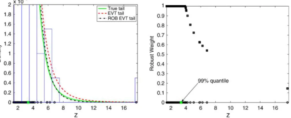
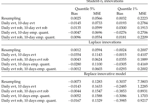
To illustrate this important point, we perform the following simple Monte Carlo experiment. We simulate 2000 observations from a Student-t5 and fix the threshold at the 0.90 empirical quantile to estimate the tail distribution. Left graph in Figure1 shows estimation results. The classical EVT method clearly overes-timates the whole tail distribution, which is highly affected by a few relatively large observations that indeed do not fit well within the chosen parametric model. The robust EVT estimator introduced in Equations (14) and (15) below produces a

Figure 1 Left graph: estimated right tail of Student-t5distribution based on 200 observations above the 0.90 empirical quantile of an i.i.d. random sample of 2000 observations; histogram rep-resents empirical density. Right graph: robust weights in Equation (15). Circles on thex-axis rep-resent simulated Student-t5observations above the 0.90 empirical quantile.

(13)

much better GPD estimate for the true tail distribution. This is illustrated also by the right graph in Figure1, which presents the robust weight of each observation implied by this estimator. These weights automatically downweight the observa-tions that are less well captured by the GPD tail. Intuitively, they identify some observations that are too influential in the score function (12) of the classical GPD estimator when compared to the other tail observations. Given that sgpd(x;ζ)is unbounded in x, these observations have a strong impact on the classical EVT estimator, inflating the overall tail estimation.

The robust EVT estimator is defined as follows. Given positive constantcgpd>

√

2, robust estimator of GPD parameters,q, is defined by (Dupuis 1999)

EG∗[ψc(sgpd(X;q(G∗)))] =0, (14)

wheresgpd(x;ζ)is the GPD score function (12) and

ψc(sgpd(X;ζ)):=A(ζ)(sgpd(X;ζ)−τ(ζ))w(X;ζ),

w(X;ζ):=min(1,cgpdkA(ζ)(sgpd(X;ζ)−τ(ζ))k−1). (15) MatrixA(ζ)and vectorτ(ζ)are solutions of the equations

Eζ0[ψc(sgpd(X;ζ0))ψc(sgpd(X;ζ0))>] =I

Eζ0[ψc(sgpd(X;ζ0))] =0.

Figure 1 shows that the robust estimator provides a nearly perfect tail estima-tion. This result is achieved by automatically downweighting only a few outlying observations, using the weighting functionw(X;ζ)in Equation (15); see right graph in Figure1. Only observations above the 0.99 quantile are downweighted, but the larger the tail observation, the lower the robust weight.5

The previous discussion is further supported by the following Monte Carlo simulation. We generate 1000 samples of 2000 i.i.d. observations each from a Student-t5 distribution, resembling model residual distributions. Using different threshold levels, we estimate the 0.99 quantile of the t5-distribution applying (i) the empirical quantile (HS), (ii) theHill(1975) estimator, (iii) the classical EVT, and (iv) the robust EVT method.

The simulation allows us to study the precision of quantile estimates and the sensitivity of classical and robust procedures with respect to threshold lev-els. The choice of threshold level plays a key role in EVT applications because it determines the trade-off between variance and bias of GPD parameter estimates.6

5_{Several authors have emphasized the instability of PML estimates of GPD when a moderate number of} influential points is present in the sample; see, for instance,Cowell and Victoria-Feser(1996) andJu´arez and Schucany(2004).

6_{A too high threshold results in too few exceedances and hence high-variance estimators. A too low} threshold induces biased estimates as the approximation implied by limit result in Equation (13) can imply large errors.

(14)

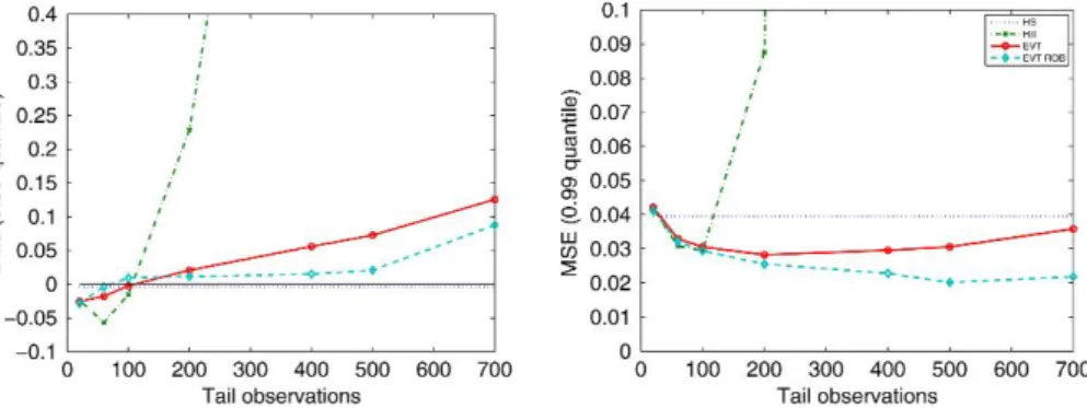
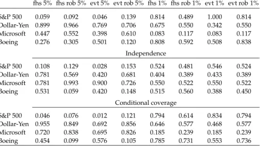
Figure 2 Estimated bias and MSE for various estimators of the 0.99 quantile of a Student-t5 dis-tribution based on an i.i.d. sample of 2000 data points using different threshold levels, that is, numbers of tail observations.

Figure2shows bias and MSE of estimated 0.99 quantile for the four tail estimators, as a function of the chosen threshold level (number of observations in the tail). By definition, the empirical quantile does not depend on thresholds but is gen-erally inaccurate. The Hill estimator is the most sensitive to the threshold level, making its empirical application rather delicate.

The robust EVT method has the lowest MSE for most threshold levels and outperforms classical EVT method consistently. For example, fixing the threshold at 0.90 quantile, that is, using 200 tail observations, classical EVT quantile estimates have MSE 11% larger than robust estimates. For lower thresholds, that is, using more tail observations, classical EVT estimates deteriorate rapidly, while robust EVT estimates are even more accurate in terms of MSE. Both in terms of bias and MSE, accuracy of robust EVT estimates is least sensitive to threshold levels among tail estimators. This is certainly a desirable property of robust EVT method because it is difficult to select thresholds optimally in empirical applications.7

In the following Monte Carlo experiments and empirical applications, we take the empirical 10th and 90th quantiles of model residual distributions as threshold levels for estimating lower and higher quantiles, that is, using 200 tail observa-tions. Such a threshold choice is the one suggested by McNeil and Frey(2000) for the classical EVT method and achieves a minimal MSE for this method in the Monte Carlo simulation of Figure2. The lowest MSE of the robust EVT method is achieved at a lower threshold level (see Figure2). Therefore, the VaR forecasting performance of robust EVT could be in principle further improved by considering different choices of the threshold level. We do not investigate this issue in more detail in the sequel.

7_See_{McNeil and Frey}_{(2000) and}_{Gonzalo and Olmo}_{(2004) for further evidence on the choice of the} threshold level.

(15)

1.5 Choice of Robustness Tuning Constants

The tuning constantscandcgpdin the estimating Equations (5) and (14) control for the degree of robustness of GARCH and GPD estimators, respectively. Following Mancini, Ronchetti, and Trojani(2005), we set such constants to achieve a given asymptotic efficiency under parametric reference modelsP_θ₀andG_ζ₀. The relative

efficiency of the robust estimatorais measured as trace(V(s; ˆθn))/trace(V(ψc; ˆˉθn)), where V(s; ˆθn)andV(ψc; ˆˉθn)are the asymptotic covariance matrices of the PML and robust estimators, respectively. Relative efficiencies of robust estimators are presented in Mancini and Trojani (2010). For instance, the choice c= 11 implies approximately 98% asymptotic relative efficiency. The relative efficiency of qis computed analogously.

2 MONTE CARLO SIMULATION

PML GARCH Robust GARCH

Empirical dist. fhs fhs rob

PML GPD evt —

Robust GPD — evt rob

The panel above summarizes the four VaR prediction methods studied here. For brevity, the method based on nonparametric residual bootstrap is called fhs. When GARCH dynamics are estimated using the robust estimator (5), we call this method fhs rob; evt rob uses robust estimators both for GARCH dynamics and GPD tail estimations; evt uses PML estimators at both stages. The simulation design al-lows to evaluate the contribution of each robustification step to the accuracy of VaR predictions. Comparing fhs and fhs rob, VaR predictions allows to assess the potential improvement of VaR forecasts due to robust instead of PML estimation of the GARCH model. In Section2.4, we compare VaR forecasts using true GARCH parameters. In that setting comparing evt and evt rob allows to assess the poten-tial improvement of VaR forecasts due to robust instead of PML estimation of tail distributions.

We compute out-of-sample VaR forecasts at 1% and 5% confidence levels and horizonsh = 1 day andh = 10 days, under an AR(1), asymmetric GARCH(1,1) model for daily returns. We simulate the following dynamics forY:={Yt}t∈Z: 1. Student-t5 innovation model. In this experiment, innovation in model (1) is

given by

Zt= ((ν−2)/ν)1/2Tν, (16) where random variableTνhas a Student-tdistribution withν= 5 degrees of freedom. Hence,Zt∼ i.i.d.(0, 1)and model (1) is dynamically correctly speci-fied.

(16)

2. Laplace innovation model.Innovation in model (1) is given by

Zt=2−1/2L, (17)

where random variableLhas a Laplace (or double exponential) distribution. Such a distribution has a symmetric convex density and displays fatter tails than thet5-distribution. Also, in this experiment,Zt∼i.i.d.(0, 1), and model (1) is dynamically correctly specified.

3. Replace innovative model.In this model,Y:={Yt}t∈Zis generated as follows:

Yt= (

ρ0+ρ1Yt−1+εt, with probability 1−κ, ˇ

Yt, with probabilityκ, (18)

where ˇYt ∼ N(0,$2),εt ∼ N(0,σ_t2)andσ_t2 is given by Equation (9). At time t, there is a probabilityκthat observationYtis not generated by the GARCH dynamic. The possible “shock,” ˇYt, will affect future realizations of the pro-cess mainly by “inflating” the conditional variance on subsequent days. In this experiment, model (1) is “slightly” misspecified as the dynamic Equations (8) and (9) are not satisfied for everyt. We setκ=0.2% and$=10. The probabil-ity of contamination,κ, is very low and implies (on average) four contaminated observations out of 2000 observations. The choice for $allows us to compare the accuracy of the different VaR estimators under very infrequent, but dra-matic, (symmetric) shocks. Such shocks could occur over short time periods in real data, as, for instance, in daily equity returns.

We set the AR(1), asymmetric GARCH(1,1) model parameters toρ0 = ρ1 = 0.01,

α0 = 0.03, α1 = 0.02, α2 = 0.8, and α3 = 0.2. This parameter choice reflects somehow parameter estimates typically obtained for daily percentage index or exchange rate returns; see, for instance, Bollerslev et al. (1994). At the reference modelP_θ₀, annualized volatility ofYtis about 12%. The robust GARCH estimators have tuning constantsc = 11. The robust GPD estimator hascgpd = 8. The sam-ple sizeT= 2000. Each model is simulated 1000 times. For each simulated sample path, we use the VaR prediction methods (fhs, fhs rob, evt, and evt rob) to compute VaR forecasts. In the financial industry, virtually only out-of-sample VaR forecasts are required, and in-sample measurements of VaR are far less important. In our simulations and empirical applications, all VaR forecasts are out-of-sample ones.

2.1 GARCH Dynamics Estimation

Bias and MSE of PML and robust estimators for the AR(1), asymmetric GARCH(1,1) model (8)–(9) are reported in Mancini and Trojani (2010). Estima-tion results for the robust estimatoratrunc (withl = 30 lags) discussed in Foot-note3are also reported in the appendix. Under reference modelP_θ₀, i.e., when

GARCH residuals are Gaussian, PMLE (that is indeed MLE) is only slightly more efficient than the robust estimators, a and atrunc. In all other experiments, both

(17)

robust estimators always outperform classical PML estimator in terms of MSEs, es-pecially under the replace innovative model. The overall performances of the two robust estimatorsaandatruncare very close butahas somewhat lower MSEs. The last finding supports the application of a for estimating GARCH-type models.

2.2 VaR Violation

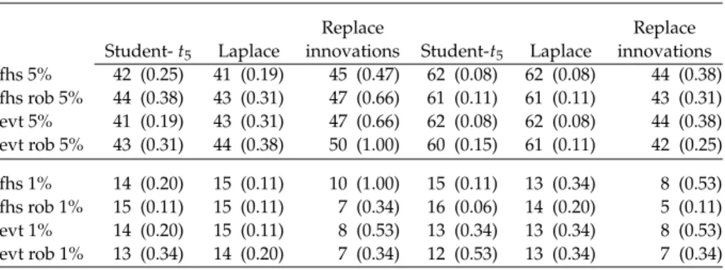
Standard analysis of VaR prediction methods is based on violation tests. In the ith simulation, a violation occurs when the actual loss is larger than the predicted VaR, that is,I(i):=1{yT,T+h(i)<yˆαT,T+h(i)}=1 and 0 otherwise. Under the null hypothesis that VaR is correctly estimated, the test statistic∑1000_i=₁ I(i)is binomially distributed as the 1000 simulations are independently drawn for both horizons h= 1 day and 10 days. Forα = 0.05 and 0.01, the expected number of violations are 50 and 10, and two-side confidence intervals at 95% level are[37, 64]and[4, 17], respectively. Table2shows number of violations for fhs, fhs rob, evt, and evt rob. All methods exhibit numbers of violations within such confidence intervals, but it is known that violation tests have typically low power. Table 2also hints some differences among VaR prediction methods. In the first two Monte Carlo experi-ments (Student-t5and Laplace innovations), only evt rob never exhibitsp-values below 0.10, even though estimated GARCH models are correctly specified. These results suggest that evt rob can outperform other approaches even in setups rela-tively favorable to classical methods, but this phenomenon is not clearly detected by violation tests. Next section studies the precision of VaR forecasts, which is a key issue for measuring market risk.

Table 2 Number of violations under different simulation models. In parentheses

two-sidep-values for null hypothesisH0: number of violations equals to the expected

num-ber of violations, that is, 50 and 10 for 5% and 1% confidence levels, respectively h= 1 day ahead VaR forecasts h= 10 days ahead VaR forecasts

Replace Replace

Student-t5 Laplace innovations Student-t5 Laplace innovations

fhs 5% 42 (0.25) 41 (0.19) 45 (0.47) 62 (0.08) 62 (0.08) 44 (0.38) fhs rob 5% 44 (0.38) 43 (0.31) 47 (0.66) 61 (0.11) 61 (0.11) 43 (0.31) evt 5% 41 (0.19) 43 (0.31) 47 (0.66) 62 (0.08) 62 (0.08) 44 (0.38) evt rob 5% 43 (0.31) 44 (0.38) 50 (1.00) 60 (0.15) 61 (0.11) 42 (0.25) fhs 1% 14 (0.20) 15 (0.11) 10 (1.00) 15 (0.11) 13 (0.34) 8 (0.53) fhs rob 1% 15 (0.11) 15 (0.11) 7 (0.34) 16 (0.06) 14 (0.20) 5 (0.11) evt 1% 14 (0.20) 15 (0.11) 8 (0.53) 13 (0.34) 13 (0.34) 8 (0.53) evt rob 1% 13 (0.34) 14 (0.20) 7 (0.34) 12 (0.53) 13 (0.34) 7 (0.34)

(18)

2.3 Accuracy of VaR Prediction

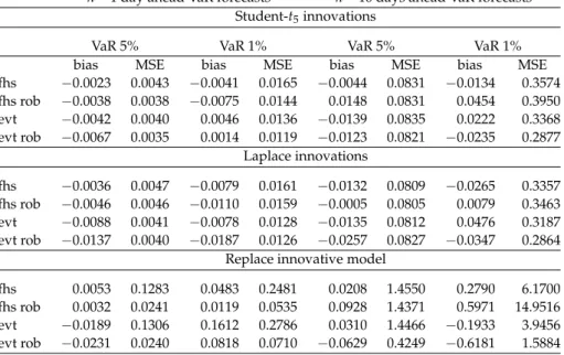
Left panel in Table3shows bias and MSE of 1-day ahead VaR predictions. In all Monte Carlo experiments, robust versions of FHS and EVT methods have smaller MSEs than corresponding classical versions. The reduction in MSE is small in the Laplace innovation model but reaches about 80% in the contaminated replace innovative model. In almost all cases, evt rob has the lowest MSE, often by sev-eral times. To gauge economic differences among VaR prediction methods, we can compare nominal and effective coverage of predicted VaR. Under the Student-t5 model, for example, a $100 value portfolio withμt = 0.01 andσt = √0.375 has a daily VaR at 1% of $2.05. If the true VaR is underestimated by $0.12, which is approximately one root MSE in the Student-t5 simulation (i.e., 0.12 ≈ √0.015), the predicted VaR of $1.93 cannot attain the perfect coverage of 1% but is violated with a sufficiently close probability of 1.2%. Hence, under this model, all VaR pre-diction methods give economically sensible VaR prepre-dictions. Similar conclusions hold for the Laplace model. However, under replace innovative model (18) un-derestimating the true VaR by $0.53 or $0.27, that is, one root MSE of evt and evt rob methods, respectively, implies substantially different situations. In the evt case, predicted VaR at 1% is indeed violated with a probability of 6.8%, while in the evt rob case only with a probability of 2.8%, and this difference is economically sizable. To further understand the magnitude of MSEs, we can standardize them by true

Table 3 Bias and MSE of classical and robust, FHS and EVT VaR prediction methods

forh= 1 day, 10-day ahead and confidence levelsα= 5%, 1% under different simulation

models

h= 1 day ahead VaR forecasts h= 10 days ahead VaR forecasts Student-t5innovations

VaR 5% VaR 1% VaR 5% VaR 1%

bias MSE bias MSE bias MSE bias MSE fhs −0.0023 0.0043 −0.0041 0.0165 −0.0044 0.0831 −0.0134 0.3574 fhs rob −0.0038 0.0038 −0.0075 0.0144 0.0148 0.0831 0.0454 0.3950 evt −0.0042 0.0040 0.0046 0.0136 −0.0139 0.0835 0.0222 0.3368 evt rob −0.0067 0.0035 0.0014 0.0119 −0.0123 0.0821 −0.0235 0.2877 Laplace innovations fhs −0.0036 0.0047 −0.0079 0.0161 −0.0132 0.0809 −0.0265 0.3357 fhs rob −0.0046 0.0046 −0.0110 0.0159 −0.0005 0.0805 0.0079 0.3463 evt −0.0088 0.0041 −0.0078 0.0128 −0.0135 0.0812 0.0476 0.3187 evt rob −0.0137 0.0040 −0.0187 0.0126 −0.0257 0.0827 −0.0347 0.2864

Replace innovative model

fhs 0.0053 0.1283 0.0483 0.2481 0.0208 1.4550 0.2790 6.1700 fhs rob 0.0032 0.0241 0.0119 0.0535 0.0928 1.4371 0.5971 14.9516 evt −0.0189 0.1306 0.1612 0.2786 0.0310 1.4466 −0.1933 3.9456 evt rob −0.0231 0.0240 0.0818 0.0710 −0.0629 0.4249 −0.6181 1.5884

(19)

unconditional variances. In the first two experiments, unconditional daily variance of percentage returns is 0.375. Hence, an MSE of 0.015 for VaR at 1% level amounts to only 4% of the unconditional variance. Under replace innovative model, MSEs of evt and evt rob are 49% and 12% of the unconditional variance (that is equal to 0.574), respectively, suggesting that evt rob provides much more accurate VaR predictions.

Right panel in Table3shows the accuracy of VaR predictions ath = 10 days ahead horizon. In the first two experiments, the dynamic model (1) is correctly specified and all VaR prediction methods tend to perform similarly in predicting VaR at 5% level, although evt rob outperforms all other methods in predicting VaR at 1% level. In the third experiment, the dynamic model (1) is slightly misspeci-fied and both FHS methods perform very poorly, with fhs rob having the largest MSE for VaR predictions at 1% level. At first sight, the last finding might appear puzzling given the higher accuracy of robust GARCH estimates; see Mancini and Trojani(2010). This result is explained by the low BP of VaR predictions based on nonparametric residual bootstrap.8 _{This point is discussed in Section} _2.4_below.

In terms of MSE, evt rob largely outperforms all other methods. For example, un-der replace innovative model, the ratio of MSE of VaR forecasts at 1% level over 10-day unconditional variance is 69% for evt and 28% for evt rob, con-firming that evt rob provides economically large improvements in VaR predictions.

2.4 Bootstrap Breakdown Point and Quantile Estimates Accuracy To disentangle the contribution of nonparametric, PML and robust EVT tail estima-tion to VaR predicestima-tions, we repeat the previous Monte Carlo simulaestima-tion using true GARCH parameters. We also investigate theoretical predictions of Equation (10) on BPs of bootstrap quantiles.

We estimate 5% and 1% quantiles (i.e., VaR) of 10-day ahead return distribu-tion. As GARCH parameters are not estimated, classical and robust FHS methods coincide, and we call them “resampling” in this section. We consider dif-ferent ways of implementing semiparametric bootstrap methods using EVT. We make an additional distinction depending on whether the quantile of simulated 10-day ahead distribution is estimated nonparametrically or using a GPD (PML or robust) estimator. This distinction highlights the additional contribution of para-metric GPD over nonparapara-metric tail estimations in producing accurate VaR forecasts. We compute VaR predictions using the following five methods:

1. Resampling (i.e., FHS method).

2. EVT applied to both daily returns and simulated 10-day ahead returns.

8_{To raise the BP of nonparametric bootstrap quantiles,}_Singh_{(1998) suggests to winsorize the data before} bootstrapping. We winsorized innovations at 0.5% and 1% levels, respectively, and then we computed 10-day ahead VaR predictions using fhs and fhs rob. MSEs of the winsorized VaR predictions did decrease but only by a small amount and the results are not reported.

(20)

3. Robust EVT applied to both daily returns and simulated 10-day ahead returns.

4. EVT applied to daily returns, and empirical quantile of 10-day ahead return distributions.

5. Robust EVT applied to daily returns, and empirical quantile of 10-day ahead return distributions.

Table4reports simulation results for the five methods under the previous Monte Carlo experiments. All MSEs of VaR forecasts in Table 4 are lower than those in Table3 as variability deriving from estimation of GARCH parameters is ab-sent now. In the first two experiments (Student-t5 and Laplace innovations), the data-generating processes do not produce “outliers.” For 5% quantiles, resampling procedures and robust EVT perform well, but classical EVT method is the least precise. For 1% quantiles, robust EVT methods have uniformly higher accuracy. Therefore, the misspecification of the GPD tail in these Monte Carlo experiments produces a quite favorable trade-off for using our robust methods in estimating the true tail of GARCH residuals.

Table 4 Bias and MSE of quantile estimates for resampling (first row); EVT applied to daily and 10-day ahead returns (second row); robust EVT applied to daily and 10-day ahead returns (third row); EVT applied to daily returns and empirical quantile of 10-day ahead returns (fourth row); robust EVT applied to daily returns and empirical quantile of 10-day ahead returns (fifth row), under different simulation models

Student-t5innovations

Quantile 5% Quantile 1%

Bias MSE Bias MSE

Resampling 0.0025 0.0566 0.0032 0.2223 Daily evt, 10-day evt −0.0145 0.0733 0.0193 0.2784 Daily evt rob, 10-day evt rob 0.0135 0.0599 0.0300 0.1913 Daily evt, 10-day emp. quant. −0.0047 0.0696 −0.0276 0.2706 Daily evt rob, 10-day emp. quant. 0.0096 0.0554 0.0181 0.2209

Laplace innovations

Resampling 0.0012 0.0594 −0.0024 0.2007 Daily evt, 10 days evt −0.0354 0.1143 −0.0015 0.4107 Daily evt rob, 10 days evt rob 0.0043 0.0624 0.0355 0.1889 Daily evt, 10 days emp. quant. −0.0280 0.1100 −0.0305 0.4169 Daily evt rob, 10 days emp. quant. −0.0012 0.0603 0.0293 0.2002

Replace innovative model

Resampling −0.0073 0.1283 0.3037 7.3803 Daily evt, 10 days evt −0.0143 0.1633 −0.2485 1.2285 Daily evt rob, 10 days evt rob −0.0044 0.1547 −0.3853 0.8931 Daily evt, 10 days emp. quant. 0.0052 0.1588 −0.3086 1.1703 Daily evt rob, 10 days emp. quant. −0.0167 0.1329 −0.3985 0.9217

(21)

Under the replace innovative model, resampling method breaks down in the estimation of 1% quantile, whereas it produces accurate results in estimating 5% quantile. From Table 1, the BP of VaR at 5% level corresponds to 0.51% outliers in the data, whereas the BP of VaR at 1% level is 0.10%. Hence, as predicted by Equation (10),κ= 0.20% of outliers in the data breaks down VaR predictions at 1%, but not at 5% using nonparametric residual bootstrap.9_{For quantile at 1% level, the}

ratio of MSE over 10-day unconditional variance is 129% for the resampling method (FHS), and only 16% for the robust EVT method applied to both daily and 10-day returns, confirming that robust EVT provides economically large im-provements in predicting VaR. Overall, robust EVT tail estimation is particulary important when forecasting VaR at low confidence levels and/or data are contam-inated by outliers.

To further understand the impact of PML and robust GARCH estimates on VaR predictions, we repeated the Monte Carlo simulation, but for comparison and to regularize the bootstrap procedure, we always fitted the tails of daily innovation distributions (and 10-day ahead returns) with the classical EVT method. Unreported results confirm that VaR predictions based on robust GARCH estimates are still more accurate than VaR predictions based on PML GARCH es-timates especially for the 10-day horizon and in the presence of outlying observa-tions. This finding suggests that robust GARCH estimates contributes significantly to the accuracy of VaR forecasts.

3 REAL DATA ESTIMATION AND BACKTESTING

We backtest VaR prediction methods on four historical series of daily rate of re-turns: S&P 500 index price from December 1988 to July 2003, Dollar-Yen exchange rate from January 1986 to January 2005, Microsoft share price from March 1986 to January 2005, and Boeing share price from January 1980 to January 2005. The data are downloaded from Datastream. Denote byy1, . . . ,yNthe historical series of returns, where, for example, N= 4500. To backtest, for example, evt rob method we proceed as follows. We usen= 2000 returns, that is, about eight years of daily data, to estimate the AR(1), asymmetric GARCH(1,1) model with the robust es-timator Equation (5) and tuning constant c = 8. Return innovation distribution is estimated using the filtered return innovations, ˆz1, . . . , ˆzn, and the robust EVT approach discussed in Section1.4, withcgpd = 6 for robust GPD estimator Equa-tion (14).10_{For day}_T ₌ _n_{, out-of-sample VaR forecasts, ˆ}_yα

T,T+h, are computed at horizonsh= 1 day, 10 days, and confidence levelsα= 1%, 5%, using the semipara-metric residual bootstrap discussed in Section 1.3. Left tail of simulated 10-day

9_{This finding also appears in the right panel of Table}_3.

10_{Considering the “noisier” nature of real data, as opposed to simulated data, and the different} characteris-tics of financial time series (indexes, stocks, and exchange rates) used in backtesting, we take a somewhat more conservative viewpoint setting the robustness tuning constantscandcgpdto lower levels than in the Monte Carlo study.

(22)

ahead return distribution is fitted using robust GPD estimator to calculate VaRs. The VaR prediction is calculated for each dayT∈ T ={n,n+1, . . . ,N−h}using a moving time window ofnhistorical returns for filtering returns and estimating distributions. GARCH estimates, however, are updated only every 500 days. The other three VaR prediction methods are similarly backtested: fhs and fhs rob rely on nonparametric rather than semiparametric residual bootstrap; evt uses PML rather than robust GARCH estimation.

For comparison, we also include (i) Historical Simulation HS; (ii)RiskMetrics (1995) (RM); (iii)Engle and Gonzalez-Rivera(1991) semiparametric GARCH model (EGR); (iv)Engle and Manganelli(2004) CAViaR model;11_{and for 10-day ahead}

VaR predictions, (v) GARCH model applied directly to 10-day asset returns. The HS and RM methods are popular in financial industry. The EGR approach provides flexible and efficient estimates of semiparametric GARCH models. The CAViaR model offers a challenging benchmark for VaR predictions, which estimates VaR directly using quantile regressions.12

3.1 Data and GARCH Estimation

Table5shows summary statistics for the daily rate of returns. The different charac-teristics of assets make the backtesting exercise particularly interesting. For exam-ple, Dollar-Yen exchange rates have large skewness and Microsoft returns large kurtosis. PML and robust estimates of AR(1), asymmetric GARCH(1,1) models for the different financial assets are collected inMancini and Trojani (2010). In several occasions and especially for the volatility parameters, the two estimates are rather different. Next sections show how these estimates induce different VaR forecasts.

3.2 Backtesting VaR Prediction

To assess the forecasting performance of the VaR prediction methods, we adopt the testing framework proposed by Christoffersen (1998). This framework con-sists of three tests and has become a standard setting for evaluating out-of-sample forecasts. We refer the reader toChristoffersen(2003, Chapter 8) for an in-depth description of the tests; a short description is also available inMancini and Trojani (2010). The test of unconditional coverage checks whether or not the overall num-ber of violations is statistically acceptable. The test of independence aims at

11_{Engle and Manganelli}_{(2004) find that empirically Asymmetric Slope and Indirect GARCH CAViaR} mod-els tend to outperform other CAViaR specifications. Given the asymmetric impact of positive and nega-tive returns on volatility (and possibly on quantiles) documented in our sample, we use the asymmetric slope CAViaR model in our empirical analysis. The Matlab code for the CAViaR model is freely available at Simone Manganelli’s webpage,http://www.simonemanganelli.org.

12_{Koenker and Bassett}_{(1978) introduce quantile regression methods; see also}_{Foresi and Peracchi}₍₁₉₉₅₎ andPeracchi(2002). From a robustness perspective, drawbacks of quantile regression is its behavior under heteroscedasticity and the nonrobustness to leverage points; seeKoenker and Bassett(1982).

(23)

Table 5 Summary statistics for the daily rate of returns in percentage: S&P 500 index price from 12/88 to 7/03; Dollar-Yen exchange rate from 1/86 to 1/05; Microsoft share price from 3/86 to 1/05; and Boeing share price from 1/80 to 1/05

Sample size Mean Std. Skew. Kurt. Min Max S&P 500 3799 0.034 1.029 −0.163 7.137 −7.113 5.573 Dollar-Yen 4969 0.016 0.688 0.496 7.596 −3.505 6.795 Microsoft 4918 0.146 2.565 −0.228 12.223 −31.111 19.552 Boeing 6535 0.055 1.938 −0.052 8.388 −17.625 15.347

verifying possible clusterings of violations over time. The test of conditional cov-erage checks in which respect the time series of VaR violations does not satisfy the correct conditional coverage.

Tables6,7, and8show number of violations andp-values of unconditional, in-dependence and conditional coverage tests for 1-day ahead VaR forecasts.13_Only

evt rob passes all violation tests with p-values above 0.10. Nearly all other meth-ods fail both unconditional and conditional coverage tests for the S&P 500 back-testing. For instance, in the conditional coverage test and VaR predictions at 5%, fhs has ap-value of 0.046, fhs rob of 0.076, EGR of 0.035, evt and CAViaR of 0.012, and HS below 0.001. Generally, HS and RM methods do not work well, especially for VaR predictions at 1% level with several p-values below 0.05. VaR prediction method based on semiparametric EGR model performs similarly to fhs method. The CAViaR model fails violation tests for the S&P 500 backtesting with most p-values below 0.05.

These empirical findings confirm the simulation results and document the accuracy of VaR predictions based on our robust approach. We now turn the at-tention to the time-series properties of VaR forecasts. Temporal profiles of VaR predictions have economic relevance because asset allocations need to satisfy VaR constraints, and VaRs determine reserve amounts to cover market risk. Asset allocations and reserve amounts cannot change heavily from one day to the next, otherwise the financial firm can incur in a variety of costs, such as transaction costs or financial losses due to liquidation of risky assets at stressed prices in high-volatile periods to reduce risk exposures. Left panel in Table10summarizes the time-series properties of VaR forecasts for Dollar-Yen backtesting. The corre-sponding statistics for S&P 500, Microsoft, and Boeing are similar and collected inMancini and Trojani(2010). In Table10, “VaR” denotes average VaR forecasts, Δaverage daily changes in VaR predictions{yˆα

T+1,T+1+h−yˆTα,T+h}T∈T,Δ2 corre-sponding empirical second moment, and|Δ|% average absolute relative changes in percentage. The last three statistics describe daily changes of VaR forecasts. In nearly all backtested time series and VaR confidence levels, evt rob has the lowest

13_{See also}_{Kuester, Mittnik, and Paolella}_{(2006) for a recent comparison of FHS methods.}

(24)

Table 6 Number of violations of classical and robust, FHS and EVT ,and HS, RM, EGR, CA V iaR, h = 1 day ahead V aR pr edictions fhs 5% fhs rob 5% evt 5% evt rob 5% Expected 5% fhs 1% fhs rob 1% evt 1% evt rob 1% Expected 1% S&P 500 108 106 109 104 90 19 21 18 19 18 Dollar -Y en 147 149 152 153 149 32 33 35 33 30 Micr osoft 155 153 156 152 146 39 38 39 38 29 Boeing 211 234 217 244 227 47 49 41 46 45 HS 5% RM 5% EGR 5% CA V iaR 5% Expected 5% HS 1% RM 1% EGR 1% CA V iaR 1% Expected 1% S&P 500 186 96 109 109 90 49 34 19 28 18 Dollar -Y en 149 151 149 148 149 31 44 32 35 30 Micr osoft 153 117 155 142 146 40 37 39 37 29 Boeing 265 206 211 237 227 66 61 47 47 45

(25)

Table 7 Likelihood ratiop-values for violations of classical and robust, FHS and EVT,

h=1 day ahead VaR predictions

Unconditional coverage

fhs 5% fhs rob 5% evt 5% evt rob 5% fhs 1% fhs rob 1% evt 1% evt rob 1% S&P 500 0.059 0.092 0.046 0.139 0.814 0.489 1.000 0.814 Dollar-Yen 0.899 0.966 0.769 0.706 0.675 0.550 0.342 0.550 Microsoft 0.447 0.552 0.398 0.610 0.083 0.117 0.083 0.117 Boeing 0.276 0.305 0.501 0.120 0.808 0.592 0.508 0.838 Independence S&P 500 0.108 0.129 0.028 0.153 0.524 0.481 0.546 0.524 Dollar-Yen 0.781 0.569 0.420 0.681 0.404 0.389 0.433 0.389 Microsoft 0.781 0.993 0.900 0.726 0.550 0.522 0.550 0.522 Boeing 0.531 0.059 0.420 0.148 0.515 0.560 0.388 0.450 Conditional coverage S&P 500 0.046 0.076 0.012 0.121 0.794 0.614 0.834 0.794 Dollar-Yen 0.955 0.849 0.692 0.856 0.646 0.577 0.468 0.577 Microsoft 0.720 0.838 0.695 0.826 0.185 0.239 0.185 0.239 Boeing 0.454 0.099 0.576 0.105 0.785 0.731 0.553 0.736

values ofΔ2_and_|_Δ_|_{%, implying smoothest VaR profiles over time. For instance, for} VaR at 5% level in the Dollar-Yen backtesting,|Δ|% for evt is 13% larger than those for evt rob. Using robust VaR predictions, the financial firm can adjust portfolio risk exposures to VaR limits more smoothly and thus more efficiently.

The empirical analysis of 10-day ahead VaR forecasts confirms and further strengthens the previous findings. Table 9shows number of violations of 10-day ahead VaR forecasts and robust Newey and West (1987) two-side p-values for the null hypothesis that the given method predicts VaR correctly.14 _{The lowest}

p-value for evt rob is 0.28. All other FHS methods are too conservative in predict-ing VaR at 5% level for the Boepredict-ing backtestpredict-ing, with p-values below 0.07. VaR pre-diction method denoted by h-ret applies fhs method directly to nonoverlapping 10-day returns. Hence h-ret avoids the resampling procedure to simulate daily returns up to 10-day horizon and relies on the empirical quantile of estimated 10-day return innovations to predict VaR. CAViaR model is fitted to nonoverlap-ping 10-day returns as well. Both methods do not work well. They suffer the in-efficient use of available information, discarding nine out of ten observations when computing nonoverlapping 10-day returns.15 _{RiskMetrics uses the suggested}

14_{Robust standard errors are computed using Newey–West covariance matrix with}_h₋_{1 lags.}

15_{In principle, EVT methods could be applied directly to 10-day returns as well, but then the issue of} limited sample size would be even more sever. To achieve 200 data points as in our previous applications, 80 years of daily returns would be required.