Runtime Prediction for Scale-Out Data Analytics

POUR L'OBTENTION DU GRADE DE DOCTEUR ÈS SCIENCES

acceptée sur proposition du jury: Prof. P. Dillenbourg, président du jury Prof. A. Ailamaki, directrice de thèse

Prof. S. Babu, rapporteur Dr A. Balmin, rapporteur Prof. K. Aberer, rapporteur

THÈSE N

_{6629 (2015)}

ÉCOLE POLYTECHNIQUE FÉDÉRALE DE LAUSANNE

À LA FACULTÉ INFORMATIQUE ET COMMUNICATIONS

LABORATOIRE DE SYSTÈMES ET APPLICATIONS DE TRAITEMENT DE DONNÉES MASSIVES PROGRAMME DOCTORAL EN INFORMATIQUE ET COMMUNICATIONS

Suisse PAR

other people’s thinking. Don’t let the noise of others’ opinions drown out your own inner voice. And most important, have the courage to follow your heart and intuition.

—Steve Jobs

In the memory of my mother, Ilona, to my beloved father, Dumitru, to my caring siblings, Gabriela and Cristian,

and to my dearest pals, Daniel and Marina. I dedicate this thesis to them.

First and foremost, I would like to thank my advisor Anastasia Ailamaki for all the guidance and support she has given to me. Without her enthusiasm, energy, and encouragements over the PhD years this work would not be possible. I am profoundly grateful to her for encouraging me to pursue my own research ideas, for boosting my research skills through constructive feedback, and for allowing me to follow my path towards PhD. I consider myself fortunate to have received her excellent advice that shaped me as a more confident person today.

I would like to thank to all the members of my thesis committee that kindly accepted to offer their time and energy to assess my dissertation and to suggest improvements. I would like to thank Vuk Ercegovac for mentoring me during my internship at IBM Almaden, and to all the other members of the group with whom I was fortunate to discuss with. My discussions with Vuk, Andrey Balmin, and Carl-Christian Kanne contributed significantly in shaping the intern-ship project. Special thanks to Andrey Balmin and Vuk Ercegovac for the fruitful collaboration we had after the internship period. Their comments were invaluable in developing PREDIcT, the core of my thesis work.

During my last PhD years I was fortunate to collaborate with Shivnath Babu. I am so grateful for all the discussions we had, for his insightful suggestions, for his enthusiasm and for his guidance. I felt privileged to chat with him multiple times at very late hours during the night. One chapter of this thesis is done in collaboration with him.

I would like to thank to all the members of the DIAS lab for making my PhD journey an enjoyable one. I thank Thomas Heinis for his excellent advice, encouragements, and friend-ship. He kindly offered his help each time I was seeking an opinion on my work. Debabrata Dash, Verena Kantere mentored me during my first PhD year for which I am grateful. I thank Farhan Tauheed, my sleepless office mate, for tolerating me over the years and for inspiring me through his photographic work. I thank Danica Porobic and Renata Borovica-Gajic for their invaluable feedback on my research work. I would also like to thank Pinar Tözün, Manos Athanassoulis, Radu Stoica, Ioannis Alagiannis, Eleni Tzirita Zacharatou, Mirjana Pavlovic, Eri-etta Liarou, Manos Karpathiotakis, Miguel Branco, Matt Olma, Cesar Matos, Raja Appuswamy, Satya Valluri, Darius Sidlauskas, Utku Sirin for the invaluable discussions, insightful comments, and the constructive feedback on my ongoing research and on my presentations. I would like to thank Erika Raetz for helping me countlessly over the years in all the administrative

problems I faced, and Dimitra Tsaoussis Melissargos for the administrative help and for her feedback on my paper submissions.

Thank you to Daniel Lupei and to Marina Boia for the precious time spent together outdoors, indoors, or at EPFL, for all the small, very small, and tiny jokes that made me smile, for our countless debates on sports, on stand-up comedy, and on music, just to name a few, for their encouragements and moral support, and foremost, for being my best friends I could have. I have greatly enjoyed the friendship of Immanuel Trummer, Thomas Heinis, Ayush Bhandari, Lada Sycheva, Valentina Sintsova, Eleni Tzirita Zacharatou, Mirjana Pavlovic, Alina Dudeanu, Cristina Ghiurcuta, Danica Porobic, Renata Borovica-Gajic, Pinar Tözün, Denisa Ghita, Mihai Martalogu, Florin Dinu, Andrew Becker, Gregoire Devauchelle, Onur Yürüten. It was my pleasure to spend time together at joyful dinners, pancake parties, barbecues over the lake, biking trips, and hikes in the Alps. Thanks to Immanuel the abstract of this thesis is also available in German.

I would like to thank my family for their unconditional moral support and love.

Finally, I am grateful to NCCR MICS and Hasler Foundation for supporting my research activ-ity during my PhD, and to Amazon for granting me hardware resources on the Amazon Web Services infrastructure.

Many analytics applications generatemixed workloads, i.e., workloads comprised of analytical tasks with different processing characteristics including data pre-processing, SQL, and itera-tive machine learning algorithms. Examples of such mixed workloads can be found in web data analysis, social media analysis, and graph analytics, where they are executedrepetitively

on large input datasets (e.g.,Find the average user time spent on the top 10 most popular web pages on the UK domain web graph.). Scale-out processing engines satisfy the needs of these applications by distributing the data and the processing task efficiently among multiple work-ers that are first reserved and then used to execute the task in parallel on a cluster of machines. Finding the resource allocation that can complete the workload execution within a given time constraint, and optimizing cluster resource allocations among multiple analytical work-loads motivates the need for estimating the runtime of the workloadbeforeits actual execution.

Predicting runtime of analytical workloads is a challenging problem as runtime depends on a large number of factors that are hard to model a priori execution. These factors can be summarized asworkload characteristics(data statistics and processing costs) , theexecution configuration(deployment, resource allocation, and software settings), and thecost modelthat captures the interplay among all of the above parameters. While conventional cost models proposed in the context of query optimization can assess the relative order among alternative SQL query plans, they are not aimed to estimateabsoluteruntime. Additionally, conventional models are ill-equipped to estimate the runtime ofiterative analyticsthat are executed repeti-tively until convergence and that ofuser defineddata pre-processing operators which are not “owned” by the underlying data management system.

This thesis demonstrates that runtime for data analytics can be predicted accurately by break-ing the analytical tasks into multiple processbreak-ing phases, collectbreak-ing key input features durbreak-ing a reference execution on a sample of the dataset, and then using the features to buildper-phase

cost models. We develop prediction models for three categories of data analytics produced by social media applications: iterative machine learning, data pre-processing, and reporting SQL. The prediction framework for iterative analytics, PREDIcT, addresses the challenging problem of estimating the number of iterations, and per-iteration runtime for a class of it-erative machine learning algorithms that are run repetitively until convergence. The hybrid prediction models we develop for data pre-processing tasks and for reporting SQL combine the benefits of analytical modeling with that of machine learning-based models. Through a

training methodology and a pruning algorithm we reduce the cost of running training queries to a minimum while maintaining a good level of accuracy for the models.

Key words: database management systems, distributed data management, runtime

pre-diction, data analytics, MapReduce, graph analytics, Bulk Synchronous Parallel, iterative processing, complex analytics, cost model, analytical model, machine learning.

Viele analytische Anwendungen führen zu einem gemischten Workload, bestehend aus Verar-beitungseinheiten völlig unterschiedlichen Typs die zum Beispiel Datenvorverarbeitung, SQL Queries oder iterative Verfahren zum maschinellen Lernen beinhalten können. Die Analyse des Internets, die Analyse von sozialen Medien oder Graph-Analyse sind nur einige wenige Beispiele für Bereiche in denen gemischte Workloads anzutreffen sind und häufig und auf großen Datenmengen ausgeführt werden (zum Beispiel um die durchschnittliche Zeit zu berechnen, die Benutzer auf den 10 populärsten Internetseiten im englischsprachigen Raum verbringen). Horizontal skalierende Systeme genügen den Ansprüchen solcher Anwendun-gen, indem sie die Daten und Verarbeitungsschritte effizient zwischen mehreren Rechnern aufteilen. Diese Rechner müssen zuerst reserviert werden bevor sie anschliessend die ihnen zugeteilten Aufgaben gleichzeitig ausführen. Um herauszufinden, welche Rechenkapazität benötigt wird um einen gegebenen Workload innerhalb eines vorgegebenen Zeitrahmens auszuführen oder um die beste Aufteilung der vorhandenen Rechenkapazitäten zwischen unterschiedlichen Anwendungen zu ermitteln, ist es notwendig die Laufzeit einer Anwendung zu schätzen bevor die Anwendung gestartet wird.

Die Laufzeit einer analytischen Anwendung ist im Vorhinein schwierig einzuschätzen da sie von vielen Faktoren abhängt, die schwer zu modellieren sind. Diese Faktoren können grob in drei Kategorien eingeteilt werden:Workload Charakteristika(beispielsweise Statistiken die die zu verarbeiteten Daten beschreiben), dieAusführungskonfiguration(Konfiguration der verwendeten Software, Zuteilung der Rechenkapazität) und dasKostenmodel, welches das Zusammenspiel aller bisher genannten Faktoren erfasst. Kostenmodelle wie sie zur Opti-mierung von Datenbank Queries verwendet werden sind darauf zugeschnitten, alternative Verarbeitungspläne miteinander zu vergleichen aber nicht dafür geeignet, die absolute Lauf-zeit akkurat einzuschätzen. Solche Kostenmodelle sind ebenfalls ungeeignet dafür, die LaufLauf-zeit iterativer Prozesse einzuschätzen die bis zur Konvergenz wiederholt werden. Gleichfalls ist es mit solchen Kostenmodellen nicht möglich, die Laufzeit von Benutzer-definierten Funktionen einzuschätzen.

In dieser Doktorarbeit wird der Beweis erbracht, dass die Laufzeit analytischer Prozesse ak-kurat vorhergesagt werden kann, indem wir den analytischen Prozess in mehrere Phasen unterteilen und während eines Testlaufs Schlüsselstatistiken zu jeder Phase erstellen, welche dann dazu verwendet werden um phasenspezifische Vorhersagemodelle zu kreieren. Wir

ent-wickeln Vorhersagemodelle für drei Kategorien analytischer Anwendungen wie sie im Bereich der Analyse sozialer Medien auftreten: iterative Verfahren zum maschinelles Lernen, Daten-vorverarbeitung und SQL Verarbeitung. Unser Vorhersagemodell für iterative Datenanalyse, PREDIcT, stellt sich der schwierigen Aufgabe, sowohl die Anzahl der Wiederholungen als auch die Laufzeit einer einzelnen Wiederholung vorherzusagen für eine Klasse von Algorithmen zum maschinellen Lernen, welche bis zur Konvergenz iteriert werden. Die von uns entwickel-ten, gemischten Vorhersagemodelle verbinden die Vorteile analytischer Modelle mit denen von auf maschinellem Lernen aufbauenden Modellen. Mithilfe ausgefeilter Trainingsmetho-den und eines Algorithmus zur effizienten Aussortierung suboptimaler Lösungen konnten wir die Kosten der Trainingsphase signifikant reduzieren bei weiterhin guter Vorhersagequalität.

Stichwörter: Datenbanksysteme, verteilte Datenbanksysteme, Laufzeitvorhersage,

Datenana-lyse, MapReduce, Graph-AnaDatenana-lyse, bulk synchronous parallel, iterative Verarbeitung, komplexe Datenanalyse, Kostenmodelle, analytische Modelle, maschinelles Lernen.

Acknowledgements i

Abstract (English/Deutsch) iii

1 Introduction 1

1.1 Motivating Use Cases . . . 2

1.2 Data Analytics Today . . . 2

1.2.1 Example: Pipeline of Analytical Tasks . . . 4

1.3 Prediction Challenges . . . 5

1.3.1 Iterative Analytics on BSP . . . 6

1.3.2 SQL and ETL Analytics on MapReduce . . . 6

1.4 Technical Contributions . . . 7

1.5 Thesis Outline . . . 8

2 Background 11 2.1 Distributed Processing Engines for Scale-Out Analytics . . . 11

2.1.1 MapReduce Execution Model . . . 11

2.1.2 Distributed Graph Processing . . . 13

2.1.3 Spark Processing Engine . . . 15

2.2 Estimating and Optimizing Iterative Processing . . . 16

2.2.1 Approximating and Sampling Large Graphs . . . 17

2.3 Performance Prediction for DBMS . . . 18

2.3.1 Nearest Neighbors-based Prediction . . . 19

2.3.2 Operator Level Models . . . 19

2.3.3 Progress Estimators . . . 20

2.3.4 Performance Modeling for Storage Devices . . . 20

2.4 Performance Prediction for MapReduce . . . 20

2.4.1 Self-tuning and Optimization . . . 20

2.4.2 Nearest neighbors-based prediction . . . 21

2.4.3 Resource Allocation and Scheduling . . . 22

2.5 Existing Prediction Approaches vs. Current Requirements . . . 22

2.6 Runtime Modeling: Background Concepts . . . 23

2.6.1 Runtime Modeling Overview . . . 23

2.6.3 Building a Cost Model . . . 25

2.6.4 Prediction . . . 28

2.6.5 Accuracy Metrics of Interest . . . 28

2.7 Summary . . . 29

3 Runtime Prediction for Iterative Analytics 31 3.1 Introduction . . . 31

3.1.1 Sketch of Proposed Approach . . . 32

3.1.2 Contributions . . . 34

3.2 The BSP Processing Model . . . 35

3.3 Modeling Assumptions . . . 36

3.4 PREDIcT’s Transformations . . . 36

3.4.1 Sampling Techniques . . . 37

3.4.2 Transform Function . . . 37

3.5 Model Fitting and Prediction . . . 38

3.5.1 Key Input Features . . . 38

3.5.2 Customizable Cost Model . . . 40

3.5.3 Prediction . . . 41

3.6 End-to-end Use Cases . . . 42

3.6.1 PageRank . . . 42

3.6.2 Semi-clustering . . . 43

3.6.3 Top-k Ranking . . . 44

3.6.4 Neighborhood Estimation . . . 45

3.6.5 Labeling Connected Components . . . 46

3.7 Limitations . . . 47

3.8 Experimental Evaluation . . . 47

3.8.1 Setup and Methodology . . . 47

3.8.2 Estimating Key Input Features . . . 49

3.8.3 Upper Bound Estimates . . . 52

3.8.4 Estimating Runtime . . . 53

3.8.5 Sensitivity to Sampling Technique . . . 56

3.8.6 Overhead Analysis . . . 58

3.8.7 Resource Allocation . . . 59

3.9 Summary of Related Work . . . 60

3.10 Conclusion . . . 60

4 Predicting Runtime of Data Pre-processing 61 4.1 Introduction . . . 61

4.2 Jaql . . . 63

4.2.1 Query Example . . . 63

4.2.2 Query Compilation in Jaql . . . 64

4.3 Modeling Assumptions . . . 65

4.4.1 Sketch of Proposed Approach . . . 65

4.4.2 Modeling Segment Performance . . . 66

4.4.3 Modeling Query Runtime . . . 67

4.4.4 Sources of Errors . . . 67 4.5 Experimental Study . . . 68 4.5.1 Experimental Methodology . . . 68 4.5.2 Experimental Setup . . . 69 4.5.3 Job-Level Predictions . . . 69 4.5.4 Query-Level Predictions . . . 71

4.6 Summary of Related Work . . . 72

4.7 Conclusion . . . 72

5 Runtime Prediction for Reporting SQL Analytics 75 5.1 Introduction . . . 75

5.2 Foundations and Overview . . . 77

5.2.1 Query Execution in HiveQL . . . 77

5.2.2 Problem Definition . . . 77

5.2.3 Starfish’s Limitations . . . 78

5.2.4 TITAN Overview . . . 79

5.3 TITAN Prediction Approach . . . 80

5.3.1 Modeling Assumptions . . . 80

5.3.2 Hybrid Prediction Model . . . 81

5.3.3 Localized Training based Models . . . 85

5.3.4 Global Analytical Models . . . 87

5.4 Training Methodology . . . 89

5.4.1 Query Template Pruning . . . 89

5.4.2 Synthetic Query Generation . . . 90

5.5 Translation Models . . . 91

5.5.1 Semantics . . . 91

5.5.2 Operator Phase and Data Mappings . . . 93

5.5.3 Use Cases . . . 94

5.6 Evaluation . . . 95

5.6.1 Setup and Methodology . . . 95

5.6.2 Training Models . . . 99

5.6.3 Testing Models . . . 101

5.6.4 Answering Performance Boost Questions . . . 105

5.7 Summary of Related Work . . . 106

5.8 Conclusions . . . 107

6 Conclusions 109 6.1 Summary of Contributions . . . 109

6.2 Impact . . . 110

6.3 Predictable vs. Non-Predictable Analytics . . . 112

6.4 Looking Ahead . . . 113

6.4.1 SLA Driven Job Scheduling . . . 113

6.4.2 Cost Models for In-memory Analytical Engines . . . 114

6.4.3 Sharing Cluster Resources Among Analytical Engines . . . 114

List of figures 115

List of tables 119

Bibliography 126

Predicting the runtime performance of large scale analytics is motivated by a number of data management tasks including workload optimization ([2]), resource management, and scheduling ([79, 76, 21]). At one end of the spectrum, users and application managers target to optimize the execution of their workloads such that pre-specified time constraints are met (i.e., deadlines). At the other end of the spectrum, resource providers aim to satisfy users’ requirements while improving utilization of their resources. In particular, schedulers and resource managers reduce unnecessary over-provisioning of resources through efficient prioritization of resource allocations.

Analytical workloads can be broadly classified into: i) deadline driven workloads with stringent time requirements, ii) best-effort workloads where explicit deadlines are not specified. Ideally, the scheduler interleaves the execution of the workloads such that deadlines are satisfied for the first category, and acceptable latencies are offered for the second category (e.g., Rayon scheduler [21]). Efficient resource planning is however possible only for the cases that the resources required to satisfy a particular optimization goal (e.g., deadline) are known in advance, beforethe workload execution. Therefore, a mechanism to assess the runtime performance of alternativehypothetical resource allocation configurationsis required. Query cost modeling has been studied in the context of database optimization, where the end goal is to find the query plan with the smallest execution cost. From a large set of possible query plans, the query optimizer quantifies the cost of each plan by using a set of analytical formulas that approximate the computational requirements of the plan. While query optimizers’ cost models were designed to quantify therelativeorder among alternative query plans, they are not very accurate when the goal is to estimateabsolutetime estimates (e.g., [29, 50, 6]). That is due to several factors which can be summarized as: simplification assumptions in the analytical model, inaccurate processing cost estimates, and inaccurate data statistics. For this purpose,runtime prediction modelsthat are designed from the ground up to estimate runtime performance have been proposed in the recent years.

1.1 Motivating Use Cases

Runtime prediction models have high practical applicability for answering What-If perfor-mance questions when anexecution configuration1that can satisfy user requested deadlines is sought. More recently, with the prevalence of using hardware infrastructure as a service (IaaS) for data management tasks, answeringcluster sizingquestions andfeasibility analysis

questions for hypothetical configurations became crucial ([39]). In this spectrum, questions like: "What hardware configuration and how many machine instances are needed to meet the runtime deadline of my analytical application?" are common, especially when transiting workloads from development clusters into production. Hence, a mechanism for assessing performance of alternative hypothetical configurations is required. We summarize the main use cases for runtime performance prediction bellow.

• Feasibility analysis: Given a workload of analytical queries, a plan for each query from

the workload, and an execution configuration (i.e., hardware/software configuration and deployment), will the workload complete within a pre-defined deadline? This use case occurs in scheduling and resource allocation where reserving resources over time has to be performed in advance of the workload execution.

• Workload on-boarding: Given a workload, a plan for for each query from the workload,

and an execution configuration, the runtime execution on the development cluster takesthours. What execution configuration can reduce the workload execution time to

t/2 hours?

• Performance boost: Given a workload and an execution configuration, the runtime

ex-ecution on the deployment cluster takesthours. Is there a new execution configuration that can boost the actual performance of the workload by a factor of 2x?”

1.2 Data Analytics Today

Today’s analytical requirements are complex, going beyond the traditional analytical operators used to compute statistical summaries over the input datasets [20]. Recent research shows that business intelligence moves towards includingcomplex analyticsinto the business process. In particular, data mining algorithms are often used in analytical pipelines for finding correlations in the ever increasing datasets (e.g., clustering, ranking) [44, 52]. For instance, social networks use machine learning to order stories in the user’s news feed (i.e., ranking). They also use data mining to group users with similar interests together (i.e., clustering).

Independently to the complexity of the analytical operators, data analytics can be categorized based on the query processing characteristics into: reportingqueries, andad-hoc queries. In contrast to ad-hoc queries which are exploratory, customized to the user’s immediate

1_{The execution configuration consists of a subset of the following parameters: software configuration settings,}

needs, reporting queries are mostly static, and are executed periodically on similar datasets or on different portions of the input dataset to answer pre-defined analytical questions about the operational state of a business. Hence, they open up opportunities forworkload re-optimization([37, 9]) andelastic workload deployment, where the deployment setting can be chosen such that application pre-specified time constraints are met ([39]). Table 1.1 summarizes the conceptual differences between reporting, and ad-hoc query processing.

Workload Workload Processing Data

type sub-type characteristics characteristics

reporting ETL, SQL, repetitive incremental

complex analytics updates

ad-hoc SQL, complex ad-hoc ad-hoc

analytics

Table 1.1 – Conceptual differences between reporting and ad-hoc query processing.

Within the complex analytics category, iterative processing became prevalent in the last few years partly due to the inherent iterative nature of many machine learning tasks used today in web analytics and social media (e.g., clustering, ranking, belief propagation), partly due to the prevalence of distributed graph processing engines that adopted the Bulk Synchronous Parallel (BSP) [55] or the Gather-Scatter [52] execution models. For these processing models abstractions, any algorithm is inherently iterative: it is a succession of processing steps that are executed in parallel on multiple processing nodes. The main difference between iterative processing and traditional query processing is that the iterative task is executedrepetitively

until a convergence condition is met, or a maximum number of iterations is reached. Figure 1.1 illustrates the concept of iterative processing on two input tables S, and T. In DBMS terminology, iterative processing can be interpreted as a join aggregate query among a relation that does not changeSand a relation that gets updated in each iterationT. In this thesis we consider iterative tasks that are executed on input datasets that are represented as graphs. Popular examples of iterative analytics used today in social media and web analytics include:

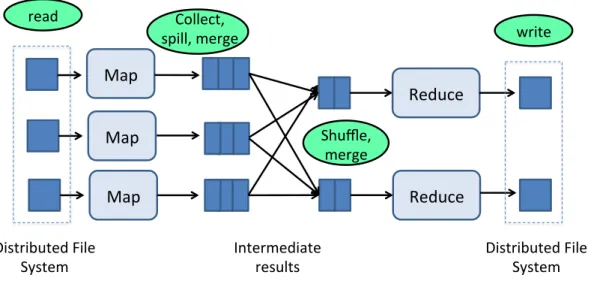
PageRank[59], Top-K ranking [45],Semi-clustering[55], statistics computation in social/web graphs (e.g.,Labeling Connected Components,Neighborhood / diameter estimation[44]). Data pre-processing tasks, commonly known as Extract Transform Load (ETL), and SQL analytics at scale are regularly executed on top of the MapReduce [23] processing engine. MapReduce is a distributed processing model that was designed to scale to thousands of commodity nodes by considering availability and fault tolerance as first class concerns. A data processing task executing in MapReduce is decomposed into a direct acyclic graph (DAG) of one or multiple MapReduce jobs. Within a MapReduce job, two processing phases exist: a

mapphase followed by areducephase. The two processing phases are parallelized by splitting the input data into partitions and by allocating multiple tasks to process the input partitions in parallel. The map tasks (i.e., the tasks executing the map phase) read, process the input partitions, and produce a set of intermediate results askey-value pairs. The reduce tasks (i.e., the tasks executing the reduce phase) aggregate all of the intermediate results with the same key generated by the map tasks and produce the final result of the MapReduce job. To tolerate

Figure 1.1 – Iterative Processing: S, input dataset that does not change as a result of executing the iterative task (i.e., input graph structure), T, input that gets updated at the end of every iteration.

failures gracefully, MapReduce stores multiple copies of the data in a distributed file system and it checkpoints intermediate results on disk at the end ofeachprocessing task. In the case of a failure only the failed task is re-executed on another machine that is available.

While MapReduce was originally designed to execute ETL tasks, it is also used to execute SQL-like analytics at scale. Several high-level, SQL-like languages have been introduced to simplify querying in MapReduce (or MapReduce-like frameworks): HiveQL[70] (Facebook), Pig Latin[58] (Yahoo!), Jaql[11] (IBM), DryadLINQ[83] (Microsoft), and others. These languages enable users to express their queries declaratively while their underlying engines automatically translate them into flows of jobs.

Compared with Pig and Jaql, HiveQL resembles the most the ANSI SQL language. HiveQL is extensively used at Facebook to execute data warehousing queries [70]. A recent study that analyses multiple production workloads from Facebook and Cloudera [18] shows that more than 50% of the total tasks execution time of the analytical workloads is spent in running HiveQL queries. Jaql and Pig provide powerful transformations on semi-structured data sets in addition to a large subset of supported SQL constructs. For instance, Jaql is actively used in the context of social media analytics, and machine learning pre-processing (e.g., summarization, cleansing, and statistics computation) [11, 63].

1.2.1 Example: Pipeline of Analytical Tasks

Figure 1.2 shows a motivating pipeline of analytical tasks in the context of web data analysis. The analytical pipeline finds the top ten best ranked pages within a web domain using a ranking algorithm, then, for each of these pages, it computes the average time the users spent

Figure 1.2 – Pipeline of Analytical Tasks in Web Data Analysis

on it during the last week. The first stage of the analytical pipeline consists of an ETL task that from a list of web pages crawled from the web extracts the hyperlinks with all the other pages (to build the web graph). Then, it filters out the pages outside of the targeted web domain. The second stage runs an iterative ranking algorithm on the input graph corresponding to the web domain. The third stage joins the output produced by the ranking algorithm with the log table that keeps statistics about page visits. Such pipelines of mixed analytical tasks (i.e., ETL, iterative ML, and SQL) are common in web analysis, blog analysis, social media analytics [82], and are executedrepetitively(e.g., every week, every month) on updated input datasets. To estimate performance of mixed analytical tasks, mechanisms for estimating the runtime of each task are required. In the following section we discuss the prediction challenges associated with each analytical task sub-category.

1.3 Prediction Challenges

Runtime prediction in a distributed setting is inherently a hard problem as runtime depends on a large number of factors that are hard to model a priori execution. Such factors include

workload characteristicsrepresented by: data statistics that determine the input processed by each database operator, and processing costs that measure the cost of executing each operator per data unit (e.g., per input tuple cost). Additional factors include the execution configuration (i.e., the resources that are allocated, the software configuration settings, the level of parallelism) and the current system state. Building highly accurate analytical models that can account for all these factors is very challenging taking into consideration the com-plexity of the modern hardware components and the comcom-plexity of the multi-layered software stack. Depending on the workload category (i.e., iterative ML, ETL, SQL), and the execution configuration used for running the workload there are different challenges for predicting the runtime. We discuss them in turn.

1.3.1 Iterative Analytics on BSP

Predicting the runtime of iterative analytics poses two main challenges that are not addressed by conventional prediction approaches proposed in the context of DBMS: i) predicting the number of iterations, and ii) predicting the processing time of each iteration. As both parame-ters depend on the characteristics of the dataset and on the convergence function, estimating their values before execution is difficult.

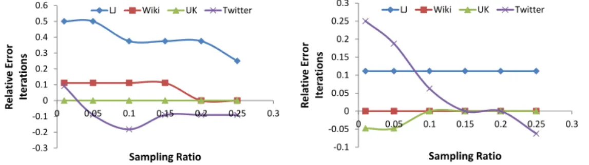
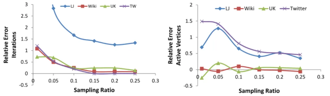
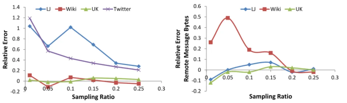
On one hand, the number of iterations depends on how fast the algorithm converges. Con-vergence is typically given by adistance metricthat measures incremental updates between consecutive iterations. Unfortunately, an accurate closed-form formula cannot be built in advance, before materializingallintermediate results. On the other hand, the runtime of any given iteration may vary widely compared with the subsequent iterations according to the algorithm’s semantics and as a function of the iteration’s currentworking set[26]: Conceptually, different code paths are executed from one iteration to the next according to the working set. Figure 1.3 shows the accuracy limitations of analytical upper bounds when estimating the number of iterations for algorithms with constant resource requirements per iteration (e.g., PageRank), and for algorithms with variable resource requirements per iteration (e.g., con-nected components). For PageRank the analytical upper bounds over-estimate the number of iterations by a factor of 2.5 on average on multiple input datasets. For connected components, analytical upper bounds over-estimate per iteration resource requirements (here, message bytes transferred) by two orders of magnitude starting from the fifth iteration.

Figure 1.3 – Using analytical upper bounds to approximate the number of iterations for PageRank algorithm (left), and per iteration resource requirements (i.e., message bytes) for connected components (right).

1.3.2 SQL and ETL Analytics on MapReduce

Cost modeling and prediction of more traditional SQL analytics is also a very challenging task as it can be seen in the large body of work carried over the past decades. While there are many analytical models proposed in the context of query optimization (e.g., [67, 54]), recent

research showed that the cost models used by query optimizers are not very accurate when the goal is to predictruntime performancemetrics [29, 50, 6]. As analytical models are aimed to assess the relative order among alternative query plans, they make simplifying assumptions about the processing costs of the operators such as: i) using aconstantper tuple cost metric, independent of the workload characteristics, and ii) disregarding the currentsystem execution state.

As a result, machine learning based approaches were proposed as an alternative approach for estimating the runtime of analytical queries (e.g., [4, 25, 29, 50, 6, 28, 63]). When using training datasets that cover the space of input queries such models are more accurate than pure analytical models as they can capture a wide range of runtime execution effects that are hard to model otherwise (e.g., interplay among workload, DBMS and underlying hardware, impact of batching). While training based prediction models can alleviate the inaccuracies introduced by simplifying modeling assumption of conventional analytical models, they have two main limitations:high re-trainingcost, which is required each time the testing workload or the execution setting changes, andreduced accuracyoutside of the training boundaries. In contrast to SQL-like analytics, modeling query runtime performance for ETL analytics on MapReduce using pure analytical models (as in traditionalquery optimization) is still an open problem. One of the main differences, is that MapReduce does not always “own" the data or the query’s operators. The input data isin-situfiles whose structure may be opaque to the system. Queries, even if written in a high-level language, often contain user defined functions (UDFs) typically written in Java. In this context, modeling the query runtime using machine learning techniques based on historical executions is more feasible.

1.4 Technical Contributions

Runtime prediction of data analytics produced by social media applications is key to facilitate feasibility analysis and cluster resource allocation as presented in Section 1.1. This thesis shows that runtime can be predicted accurately throughhybrid prediction modelsthat combine the benefits of analytical modeling with the advantages of machine learning-based models and simulation. The generic prediction methodology we develop breaks the analytical task into multiple processing phases (based on semantics), collects key input features during a reference execution on a sample of the dataset, and then uses the collected features to build

per-phasecost models. We customize this methodology for three categories of workloads: iterative machine learning, data pre-processing, and reporting SQL. We elaborate the technical contributions of this thesis bellow:

• Sampling and Input Transformations for Iterative Processing on Graphs: We develop

the set of transformations applied to the input graph dataset and to the input parameters that altogether can preserve the processing characteristics of the iterative task during a short run on sample dataset. We proposeBiased Random Jump, a sampling technique

that exploits the connectivity among highly connected nodes in scale-free graphs, and can be successfully used for prediction for a number of iterative algorithms widely used in analyzing social media data. We empirically show that the judicious choice of the sampling technique, that preserves key properties of the input dataset, altogether with input parameter transformations can be effectively used in prediction.

• Hybrid Prediction Models for Data Analytics: We design hybrid prediction models

that combine the generality of analytical models , with the power of machine learning models to exploit prior workload executions. Such a modeling design allows to estimate the runtime of both conventional SQL operators, but also the runtime ofuser defined

pre-processing tasks, and that ofiterative analyticsthat are not “owned” by the data management layer. Additionally, our contribution includes the pool of key features that we identified for each workload category.

• Training Methodology and Translation Models for Reporting SQL: We propose a

method-ology for generating training queries and a pruning algorithm that limit the number of queries used in the training workload to a minimum. The training methodology reduces the time of running the training workload from days to hours while maintaining a good level of prediction accuracy for the models. Translation models, i.e., relative prediction models that exploit prior reference executions of the query that is predicted, improve the prediction accuracy of conventional prediction models beyond the training boundaries.

1.5 Thesis Outline

In this thesis we propose performance prediction techniques forreportingqueries that include a class of iterative machine learning algorithms executing on BSP, ETL tasks expressed in Jaql, and SQL-like queries expressed in HiveQL.

The following section summarizes the contributions of the thesis and gives an overview of the next chapters.

• Background: Chapter 2 introduces general related work in the context of runtime

performance prediction for data analytics. We start with background concepts on distributed processing engines in Section 2.1. Estimation techniques and sampling for iterative processing are presented in Section 2.2. Prediction approaches for DBMS are presented in Section 2.3, while prediction approaches for MapReduce are presented in Section 2.4. Section 2.5 summarizes recent prediction approaches while illustrating their limitations. Section 2.6 presents background modeling concepts that we later use for designing prediction models for iterative analytics, data pre-processing, and reporting SQL.

• Runtime Prediction Methodology for Iterative Analytics: Chapter 3 considers the

datasets. Our main contribution for this problem is PREDIcT, an experimental method-ology that proposes a set of transformations that can be used to estimate the number of iterations and the key input features of the iterative task using a sample-run on a small sample of the input dataset. The other contribution of this chapter is the design of a framework for building customized cost models for iterative analytics executing on top of Bulk Synchronous Parallel execution model (in particular, the Apache Giraph implementation). Finally, we present a thorough performance evaluation of PREDIcT on real datasets. For a 10% sample, the relative errors for estimating key input features range in between 5%-20%, while the errors for estimating the runtime range in between 10%-30% for all the scale-free graphs analyzed.

• Runtime Prediction for Data Pre-processing (ETL Tasks): Chapter 4 tackles the

prob-lem of predicting the runtime of data pre-processing tasks. Examples of data pre-processing tasks include machine learning pre-pre-processing (e.g., data cleaning) and ETL (Extract Transform Load). In this chapter, we propose a technique that predicts the runtime performance of a class offixed queriesrunning over varying input data sets. Our approach uses minimal statistics about the input data sets (e.g., input size, tuple size, cardinality), which are complemented with historical information about prior query executions (e.g., execution time). Our experiments on real workloads show the feasibility of the approach: we obtain less than 25% relative prediction error for 90% of predictions.

• Runtime Prediction Methodology for SQL Analytics: Chapter 5 addresses the problem

of estimating the runtime of reporting SQL analytics. Starting from a prior execution of a reporting query we propose an approach for estimating the runtime of the query for other hypothetical configurations consisting of: i) query plan re-writes in terms of different operator implementation and possibly different packings of operators within one or several MapReduce jobs, and ii) a pool of potential hardware deployments. For this purpose we develop TITAN: i.e., Training Methodology and Translation Models for runtime prediction. Our contributions include a hybrid prediction approach and a train-ing methodology that altogether reduce the traintrain-ing cost of state of the art prediction approaches while maintaining a good level of accuracy for the models. Our experiments show the feasibility of the prediction approach both on private and on public clusters. The 95-percentile average relative error is less than 25% on the testing benchmarks.

• Conclusions: Chapter 6 summarizes this thesis and outlines future avenues of research

in query runtime prediction. We discuss a number of interesting topics that are worth pursuing in the context of scheduling, in-memory analytical engines, and shared infras-tructures.

In the first sections of this chapter we present related work on distributed processing engines and runtime prediction techniques applied for data analytics in general. Specific differences with respect to the prediction techniques proposed in this thesis are also summarized later in the respective chapters. In the last section of this chapter we introduce runtime modeling concepts that we use for runtime prediction in all of the following chapters.

2.1 Distributed Processing Engines for Scale-Out Analytics

MapReduce is a programming model and a framework for processing large sets of raw data. A MapReduce program consists of two functions: map and reduce. The map function process the input data and produces a set of intermediate results as key-value pairs, while the reduce function aggregates all the intermediate results with the same key to produce the final result. MapReduce framework operates in conjunction with a distributed file system, where it stores the input and output data. Input data is represented as text or key/value pairs. Hence, the burden of data parsing is passed to the user’s code. The data model allows for more flexibility as compared with state-of-the-art DBMS where the data has predefined structure, but comes at the cost of parsing the data each time a task is being executed.

Figure 2.1 illustrates the processing phases when running an analytical job on MapReduce. The job has three map tasks that read the input from the distributed file system, then apply the user defined transformations defined in the map function. Map tasks produce intermediate results as key-value pairs which are spilled to the local file system of each of the map tasks. Two reduce tasks copy the key-value pairs assigned to them based on a partitioning strategy on key, merge key-value pairs having the same key, then apply the user defined reduce function that produces the final result.

Map$

Map$

Reduce$

Map$

Reduce$

Figure 2.1 – MapReduce Execution Model: Map tasks transform the input data and output intermediate results as key-value pairs. The reduce tasks copy and merge all the values corresponding to the same key, then apply the reduce function to produce the final result.

data analytics:

• Fault Tolerance and Scalability: Designed to process large amounts of data using

thou-sands of commodity machines, MapReduce has mechanisms to tolerate failures grace-fully. MapReduce is resilient to large scale worker node failures by re-scheduling tasks on live nodes and by checkpointing intermediate results of the MapReduce job. Hence, in the case of a node failure the framework re-executes only the failed task of the MapRe-duce job.

• Elasticity: Worker nodes can be easily added in or removed. The underlying filesystem

takes care of balancing the load among all the data nodes, while computation is uni-formly balanced across all the worker nodes. Extending deployment of a traditional parallel database requires significant efforts in tuning it before actually exploiting the new hardware resources efficiently.

• Load Balancing: The MapReduce framework divides the Map and Reduce phases into a

number of pieces much larger than the number of machines such that each machine executes many different tasks. This improves dynamic load balancing and recovery. If a node fails, tasks executed on the failed node can be spread out across all the other machines. Additionally, to deal with straggler nodes (i.e., machine that is performing poorly), MapReduce schedules backup tasks. Specifically, when the job is close to completion the master node schedules backup executions for the remaining tasks. A task finishes when either the primary or backup task completes its execution.

an open source implementation that is available for free. Hadoop1is an open source implementation of the MapReduce framework.

Traditional applications of MapReduce include: ETL systems (Extract, Transform, Load) that transform data into different formats that are further consumed by other storage systems, complex analytics that cannot be expressed in SQL (multiple passes over the data: e.g., data mining, data clustering) or data analytics on unstructured data (grep, URL access frequency, inverted index).

Iterative Processing on MapReduce

Mahout[7] is a library for MapReduce that aims to scale the execution of machine learning

algorithms on large input datasets. The library includes both iterative and non-iterative algorithms. The iterative category includes: clustering (e.g., spectral, k-means, canopy) and algorithms used by recommender systems (e.g., matrix factorization, collaborative filtering). The non-iterative category includes: classification (e.g., Naive Bayes, Logistic Regression), dimensionality reduction (e.g., PCA), etc.

Pegasus[44] is a similar effort as Mahout with the difference that the project is targeting to

mine large input graphs. Pegasus proposes efficientmatrix-vector multiplicationabstractions that can be used to implement a class of graph mining algorithms on top of MapReduce engine. Examples of algorithms that benefit from such an abstraction: connected components, diameter/radius estimation, random walks, PageRank.

HaLoop[14] proposes optimization techniques when executing iterative computation on

MapReduce. As explained in Section 1.2 and illustrated in Figure 1.1, iterative processing is executed among one relation that does not change and one relation that gets updated in every iteration. The MapReduce execution model is inherently inappropriate to execute iterative processing efficiently as it requires to read both inputs at the beginning of every iteration, and additionally it shuffles and then spills intermediate results on disk. For algorithms with a large number of iterations such an execution model is very inefficient. In this context, HaLoop [14] caches invariant input datasets in memory when executing iterative algorithms on MapReduce.

2.1.2 Distributed Graph Processing

An important class of analytics today is executed on graphs. Social media analysis and blog analysis require graph processing engines that can process large data sets efficiently. Recent graph processing engines use avertex centric approach, that is, each vertex executes an in-stance of avertex programtowards implementing the graph algorithm. Concretely, each vertex executes local computation on its local data structures (state information can be associated

with the vertex and the neighboring edges), then it communicates with other vertices of the graph as needed to implement the semantics of the algorithm. The distributed algorithm implementation is in fact a succession ofiterationsthat are composed oflocal computation

andcommunication. Based on the communication and synchronization models (whether

synchronizationamong all vertex programs is enforced or not at the end of each iteration), we can classify engines into:synchronousandasynchronous. In the following, we describe Pregel [55], a synchronous graph processing engine, and GraphLab [52] an asynchronous variant.

Pregel

Pregel follows a bulk synchronous parallel (BSP) [73] processing model that uses message passing for communication. All vertices run their vertex programs in parallel for a number of iterations (aka, super-steps). Before starting a new iteration, each vertex receives all its designated messages from the other vertices that were sent in the previous iteration. At the end of an iteration, each vertex send messages to its neighbors as needed. A barrier synchronization point is enforced at the end of each iteration to ensure that all messages send in one iteration are received before starting the next iteration. Vertices that completed running their vertex program can vote to halt. By doing so they remove themselves from the list of vertices that will execute computation in the next iteration. A halted vertex that receives a message it is automatically re-started in the next superstep. The algorithm completes when there are no more messages to be sent among vertices and all vertices voted to halt. Pregel introduces the concept ofcombinerswhich are user defined function that merge messages destined to the same vertex. Combiners are required to be associative and commutative operators.

GraphLab

GraphLab builds on anasynchronous distributed shared memoryabstraction. In this pro-cessing model, vertex programs have shared access to a distributed graph. Concretely, each vertex program can access the data of its current vertex, of the neighboring vertices, and of the neighboring edges. A vertex program can be scheduled to be re-executed again (i.e., a new iteration) by itself or by its neighboring vertices through a signaling mechanism. We observe that GraphLab removes message passing interface and the synchronization point at the end of each iteration. Instead of using a barrier among all vertex programs, the underlying processing engine ensures serializability by preventing neighboring vertices (that access the same shared state) to be executed at the same time.

GraphLab introduces the Gather-Apply-Scatter (GAS) model to represent the conceptual phases of a vertex program. During the gather phase, state about adjacent vertices and edges is collected and aggregated into aggregator object. The aggregate operator can be a generalized

sumover the neighborhood of the current vertex, and it must be associative and commutative. During the apply phase the current vertex value and the aggregator value are used to update

the new vertex value. Finally, during the scatter phase the new vertex value is used to update the data on adjacent edges and vertices. We note that the scatter and gather phases control the fan-in and the fan-out of the vertex program.

PowerGraph[31] was introduced to address the challenges of power-law graphs where there

is a lot of work imbalance among vertices of the graph. In particular, power-law graphs have a small number of vertices that have much larger neighborhoods than most of the vertices of the graph. For such graphs, processing abstractions that distribute work symmetrically among vertices suffer from per iteration processing time imbalance. PowerGraph is a hybrid approach that adds parallelization within a vertex program. That is, vertices with large neighborhoods distribute the vertex program among multiple workers. PowerGraph is in fact a hybrid of GraphLab and Pregel abstractions, inheriting from GraphLab the asynchronous engine and the distributed shared memory model for data access, and from Pregel the combiner concept. PowerGraph parallelizes the gather and scatter phases of the GAS abstraction, uses a combiner to aggregate all the results created during the gather phase, then executes the apply function to update the vertex value with the aggregated result.

Other Graph Processing Engines

Other graph processing engines that optimize the runtime performance when processing large scale graphs in parallel were proposed in the recent years. Mizan [45] is a BSP graph processing engine that balances the load dynamically among workers based on performance characteristics collected at runtime. XStream [66] is a system for processing both in-memory and out-of-core graphs using a shared memory machine. GreenMarl [42] is a domain specific language abstraction and a runtime system that allows users to express their graph processing algorithms declaratively while not trading-off on the performance. The optimizer takes full control of translating the high level code into optimized code that is then executed in parallel using a distributed shared memory abstraction.

2.1.3 Spark Processing Engine

Spark [84] is an alternative MapReduce paradigm implementation that was designed for very fast computation. Spark is compatible with Hadoop’s storage API, and is on average 40x faster than Hadoop [82]. Spark develops an in-memory storage structure calledresilient distributed datasets (RDDs)for storing intermediate results. As a result of saving intermediate results on RDDs instead of saving them on disks, Spark is very efficient for iterative computation with a large number of iterations.

RDDs are a restricted form of distributed shared memory. They were designed to offer high throughput (close to the maximum given by the memory bandwidth) for coarse granularity updates. Concretely, RDDs are distributed collection of records that are immutable and cached in the memory of the cluster. They can only be built through coarse-grained deterministic

parallel transformations (e.g., map, filter, join, etc). In the case of failures, RDDs are re-built using lineage.

Shark Processing Engine for Mixed Analytics: Shark [82] is an execution engine formixed

analyticsthat supports both efficient SQL and machine learning computation at scale with

fine grainfault tolerance. Shark is essentially HiveQL on Spark and is compatible with Hive’s interfaces. Overall, Shark is in the range of (10x, 100x) faster than HiveQL on Hadoop. Besides the performance improvements due to using Spark’s resilient distributed datasets abstraction, query planning in Shark benefits from additional optimizations such as:partial DAG execution,

map pruning,efficient memory storage.

Partial dag execution: collects statistics at the runtime that are later used to select a particular join implementation (e.g., map join or shuffle join), and the degree of parallelism of the following jobs in the query DAG. For instance, based on the partition sizes fine grain partitions can be coalesced into coarse partitions. Other statistics that are collected: record counts, approximate histograms.

Map pruning: is a mechanism of pruning partitions that do not contain query results based on statistics that are collected during the data loading phase of each partition.

Efficient memory storage: Shark employs column-oriented storage using arrays of primitive types instead of storing rows as Java objects. Shark reduces the book-keeping overhead and at the same time it reduces the access time.

2.2 Estimating and Optimizing Iterative Processing

Prior work on iterative algorithms mainly focuses on providing theoretical bounds for the number of iterations an algorithm requires to converge (e.g., [46, 44, 34]) or worst case time complexity (e.g., [8]). These parameters, however, are not sufficient for providing wall time estimates due to the following two reasons: i) As simplifying assumptions about the charac-teristics of the input dataset are made, theoretical bounds on the number of iterations are typicallyloose[46, 8]. This problem is further exacerbated for a category of iterative algorithms executingsparse computation, where the processing requirements of any arbitrary iteration vary a lot as compared with subsequent/prior iterations [26, 52]. For such algorithms, per iteration worst case time complexities are impractical when the goal is to estimateactual run-time. ii) Per iteration processing runtime cannot be captured solely by a complexity formula. System level resource requirements (i.e., CPU, networking, I/O), critical path modeling and a cost model are additionally required for modeling runtime.

Iterative execution was also analyzed in the context of recursive query processing. In partic-ular, multiple research efforts [10, 3, 13] discuss execution strategies (i.e., top-down versus bottom-up) with the goal of performance optimization. Ewen et al. [26] optimize execution ofincremental iterationsthat are characterized by few localized updates, in contrast with

bulk iterations, that always update the complete dataset. Although performance optimization has an immediate impact on the runtime of the queries, the aforementioned techniques are complementary to the runtime prediction problem we study in this thesis.

2.2.1 Approximating and Sampling Large Graphs

With the goal of reducing the processing time of ever increasing input graphs, sampling and sketching techniques that canapproximatesome of the properties of the complete graph have been studied over the past recent years (e.g., [47, 48, 33, 43]). In these works, the main goal is to take a sample that can be used to approximate the result of the graph processing task. For instance, evaluating whether the input graph is connected, approximating the in/out node degree distributions, the effective diameter (i.e., 90-th percentile longest distance).

Sampling graphs had been analyzed in the context of social networks. Leskovec et al. propose sampling techniques based onrandom walks[47] with the goal of maintaining certain proper-ties on the sample such as the in/out node degree distributions, clustering coefficient, and effective diameter.

A random walk on a graph starting at a vertexvcorresponds to randomly picking an edge that starts atvand ends at one ofv’s neighboring vertices. A sampling technique based on random walk takes multiple random walks on the input graph until a certain percentage of vertices (or edges) have been sampled. There are multiple variants of sampling algorithms based on random walks. An excellent survey is that of Hu et al. [43]. In the following we summarize the best performing sampling techniques in the context of preserving connectivity, node in/out degree proportionality, and the effective diameter of the sampled graph.

• Random Walk[47]: Random Walk picks a starting seed vertex uniformly at random from

all the input vertices. Then, at each sampling step an outgoing edge of the current vertex is picked uniformly at random and the current vertex is updated with the destination vertex of the picked edge. With a probabilitypthe current walk is ended and a new random walk is started from the original seed vertex. The process continues until the number of vertices picked reaches the sampling ratio. With this sampling strategy there is a risk of getting stuck, if the starting vertex is a sink, or if it belongs to a small isolated component. If after a long number of sampling steps there is no progress in the number of picked vertices, random walk re-initializes the starting node to a new arbitrary vertex of the graph.

• Random Jump[47]: Random Jump is very similar with Random Walk. The difference

is that Random Jump re-initializes the starting node to an arbitrary vertex of the graph

each timea new random walk is started. Hence, this sampling scheme has no risk in getting stuck during the sampling process.

are known to have bias towards high degree nodes in the input graph. That is vertices with high out degree are likely to be visited more often during the sampling process than vertices with low out degree. With the goal of sampling vertices uniformly at random (i.e., with a probability of _|V1_|, where|V|the total number of vertices in the graph), Metropolis-Hastings Random Walk adjusts the transition probability within a random walk as follows: Pv,w=              1 kv × mi n(1,kv kw ), if w is neighbor of v (1− X y!=v Pv,y), if w = v

0, for any other vertex of the graph

, wherekv, andkw the out degrees of verticesv, andw. In summary, MHRW always

accepts a walk towards a vertex with a lower degree and rejects some of the moves to vertices with higher degree. Thus, it eliminates the bias towards vertices with high degree.

Sampling vs. Sketching

In the context of data streaming model, McGregor et al. proposessketchingtechniques with the goal of reducing the cost of processing large input graphs [33, 5]. Concretely, sketches reduce the algorithm processing space complexity fromO(n2) toO(n×pol yl og(n)). Sketching techniques use multiple linear projections of the input graph so that they can preserve a certain property of the original graph (such as connectivity, k-connectivity, bipartiteness) in the sketch space with high probability. Once a sketch is constructed, the algorithm is executed in the sketch space to approximate results: Given a graph processing task T, an input graph G, and a corresponding sketch S, the result of executing T on G is approximated with the result obtained by executing T on S. The main differences with sampling approaches based on random walks can be summarized as follows: i) random walk-based sampling approaches aim to preserve multiple properties of the input graph while sketching is customized to preserve only one input property with high probability. ii) random walk samples are used to summarize some of the characteristics of the complete graph whereas sketches aim to reduce the memory (space) requirements of processing large input graphs in the context ofdata streams.

2.3 Performance Prediction for DBMS

Estimating the runtime execution of analytical workloads was heavily studied in the DBMS context from multiple angles:initial runtime predictors[29, 4, 25],progress estimators[16, 53, 57], andself-tuning systems[40, 38]. Prediction approaches proposed in the DBMS context account for system level resource requirements (i.e., CPU, IO, network, memory) and use a

cost model (either analytical, based on black box modeling or a hybrid) for translating them into runtime. For instance, [29] proposes a technique to predict query performance using a cost model based on machine learning that clusters queries with similar performance based on query’s input parameters as known asinput featuresin the machine learning community.

2.3.1 Nearest Neighbors-based Prediction

Ganapathi et al. propose an approach for predicting the runtime execution of HP Neoview queries using statistical methods based on Kernel Canonical Correlation Analysis [29]. The proposed model predicts the runtime of a query based on the runtime ofmnearest neighbor queries for which performance was tracked during a training phase. For finding the nearest neighbors an n-dimensional distance metric is used (i.e., kernel), the dimension being given by the size of the feature vector. The key input features include operator types, operator counts, and input data statistics as returned from the query optimizer.

A related approach that uses linear regression to model the runtime of analytical queries was proposed by Zhu et al. in the context of Multi Database Systems [86]. The proposed method separates queries into classes according to their access methods so that the cost of the queries in each query class can be approximated by the same formula. The set of features considered are the input/output cardinalities, the size of intermediate results, the tuple length and the physical size of the input/output tables. The approach uses multi-variate linear regression to model the cost of queries.

2.3.2 Operator Level Models

Recent research introduced the idea of usingoperator levelmachine learning models [6, 50]. In particular, Akdere et al. [6] propose multiple granularity prediction models: “plan level” models, “operator level” models or hybrids of the above two with the goal of predicting the runtime of analytical queries for both static and ad-hoc workloads. Their work stresses the idea ofmodel re-usabilitythrough operator level models. While operator models are more accurate for computing the runtime of operators, they require additional modeling mechanisms for computing query level estimates (i.e., modeling the critical paths, taking into account operator pipelining).

Li et al. propose an approach for improving the prediction accuracy on testing sets outside of the training boundaries [50]. In particular, each operator is modeled through a hybrid of models with a fixed functional form and decision trees which are discrete (i.e., in particular, Multiple Additive Regression Trees). Based on the observation that models with a fixed functional form are more powerful on testing sets outside of the training boundaries, and that decision trees are more accurate when the training sets have a good coverage of the testing set, they propose a hybrid of the two.

2.3.3 Progress Estimators

A sub-class of performance estimators focuses on estimating the progress of queries at runtime (e.g., [16, 53, 57]) rather than on predicting their runtime before execution. In contrast with prediction mechanisms, progress estimators benefit from a feedback loop mechanism which can correct wrong estimates at the runtime. Similar adaptive techniques that are calibrating statistics at runtime were also proposed in the literature [69, 24]. Progress estimators do not replace the requirement for runtime predictors, as for many use cases (i.e., scheduling, resource allocation) runtime estimates are required beforethe query starts execution. In fact, runtime predictors can be used in conjunction with progress estimators to estimate the runtime of forthcoming query pipelines for which dynamic statistics (collected at runtime) are not yet available.

2.3.4 Performance Modeling for Storage Devices

Mesnier et al. [56] propose relative fitness models for storage devices that estimate perfor-mance of a workload on device D1 based on a set of features that include perforperfor-mance and resource utilization counters (in addition to the workload characteristics) corresponding to the workload execution on another device D2. The training phase consists of: i) running synthetic benchmarks on all storage devices that are representative for a large spectrum of real workloads, and ii) building pairwise models among pairs of devices that exploit correlations among performance metrics of a given workload executing on different devices. Classification and Regression Tree (CART) models are used in the model fitting phase due to their simplicity and flexibility.

2.4 Performance Prediction for MapReduce

Herodotou et al. propose Starfish [38], a self-tuning system for Extract Transform Load (ETL) workloads that uses performance models with the goal of workload tuning, in particular, finding the best set of configuration settings for a given workload and a cluster deployment. Starfish was designed to help practitioners in data analytics getting the best job performance without requiring them to know the tuning knobs of the underlying MapReduce infrastructure. The key building block for finding the best configuration settings is thejob profile, which models the processing characteristics of an input job. The processing characteristics are grouped into: processing cost factors, and data statistics. Given a MapReduce job, a job profile is taken by executing the job on asampleof the input dataset. Then, the approach uses the job’s processing characteristics from the job profile, a set of analytical models, and simulation to predict the job’s runtime for a range of input configuration settings. Starfish’s What-If engine is called for each potential input configuration, and the best configuration setting is returned to the user.

Elastisizer [39] extends Starfish’s approach for thecluster sizing problem, which stands for finding the cluster size and the type of machine instances (in terms of resource characteris-tics) that best meet the requirements of the workload. Hence, in addition to configuration settings, the search space includes cluster resources in terms of instance types on Amazon EC2. Elastisizer uses controlled black box models for estimating the processing cost factors on the target deployment. A set of synthetic workloads are generated and executed on each instance type to generate the data that is used for training. In terms of model fitting algorithm, M5 tree models [65] are used. M5 tree is a decision tree that instead of using the average of all training examples falling within a leaf node, uses a second level modeling phase among all observation falling within each leaf node. In particular, linear regression models are used to fit the observations within each node. We make several observations: Both Starfish and Elastisizeraverageprocessing cost factors among the job’s task profiles to produce areference profilethat is later used in prediction. As we later show averaging processing cost factors among tasks with very different input data properties is one source of modeling error that may cause important inaccuracies when estimating the runtime with Starfish’s analytical models. The task profiles are collected at MapReduce phase granularity and thus, do not track more specific information about the processing tasks executed within the map, and reduce functions (e.g., scan, join, project operators).

Wu et al. [80] propose analytical cost models for HiveQL operators with the underlying goal of query optimization. Their work is tailored towards reducing the size of intermediate results by adaptively grouping join operators that can be processed in one single MapReduce job. Unlike conventional optimization, the proposed optimization approach is tailored to the characteristics of MapReduce processing model such as materialization of intermediate results and data shuffling. Similarly with PostgreSQL cost model, or the query cost calibration approaches proposed for PostgreSQL [81, 68], processing cost factors are assumedconstant

for a given hardware infrastructure.

2.4.2 Nearest neighbors-based prediction

Ganapathi et al. extend their method proposed in the context of database queries [29] for HiveQL queries executing on top of MapReduce [28]. The input features used include a mix of MapReduce specific configuration settings and query features taken from the query plan. The models are built at coarse granularity (job/query granularity). The set of input features considered include configuration parameters and input data characteristics: i.e., number and location of map/reduce slots, input bytes, bytes read from local disk, bytes read from the distributed file system (i.e., HDFS in Hadoop). A large number of training queries is used for fitting the models (in the order of 1000s).