Combining high productivity and high performance in image processing using Single Assignment C on multi-core CPUs and many-core GPUs

UvA-DARE is a service provided by the library of the University of Amsterdam (http://dare.uva.nl)

UvA-DARE (Digital Academic Repository)

Combining high productivity and high performance in image processing using single

assignment C on multi-core CPUs and many-core GPUs

Wieser, V.; Grelck, C.U.; Haslinger, P.; Guo, J.; Korzeniowski, F; Bernecky, R.; Moser, B.;

Scholz, S.-B.

Published in:

Journal of Electronic Imaging DOI:

10.1117/1.JEI.21.2.021116

Link to publication

Citation for published version (APA):

Wieser, V., Grelck, C., Haslinger, P., Guo, J., Korzeniowski, F., Bernecky, R., ... Scholz, S-B. (2012). Combining high productivity and high performance in image processing using single assignment C on multi-core CPUs and many-core GPUs. Journal of Electronic Imaging, 21(2), 021116. https://doi.org/10.1117/1.JEI.21.2.021116

General rights

It is not permitted to download or to forward/distribute the text or part of it without the consent of the author(s) and/or copyright holder(s), other than for strictly personal, individual use, unless the work is under an open content license (like Creative Commons).

Disclaimer/Complaints regulations

If you believe that digital publication of certain material infringes any of your rights or (privacy) interests, please let the Library know, stating your reasons. In case of a legitimate complaint, the Library will make the material inaccessible and/or remove it from the website. Please Ask the Library: http://uba.uva.nl/en/contact, or a letter to: Library of the University of Amsterdam, Secretariat, Singel 425, 1012 WP Amsterdam, The Netherlands. You will be contacted as soon as possible.

Combining High Productivity and High Performance in

Image Processing Using Single Assignment C on

Multi-core CPUs and Many-core GPUs

Volkmar Wieser

, Clemens Grelck

, Peter Haslinger

, Jing Guo

, Filip Korzeniowski

, Robert

Bernecky

, Bernhard Moser

, and Sven-Bodo Scholz

a

_{Software Competence Center Hagenberg, Software Park 21, Hagenberg, Austria}

_{University of Amsterdam, Science Park 904, Amsterdam, Netherlands}

c

_{University of Hertfordshire, College Lane, Hatfield, United Kingdom}

d

_{Snake Island Research Inc, 18 Fifth Street, Ward’s Island, Toronto, Ontario, Canada}

_{Heriot-Watt University, Riccarton, Edinburgh, United Kingdom}

ABSTRACT

In this paper the challenge of parallelization development of industrial high performance inspection systems is addressed concerning a conventional parallelization approach versus an auto-parallelized technique. Therefore, we introduce the functional array processing language Single Assignment C (SaC), which relies on a hardware

virtualization concept for automated, parallel machine code generation for multicore CPUs and GPUs. Addi-tional, software engineering aspects like programmability, productivity, understandability, maintainability and resulting achieved gain in performance are discussed from the point of view of a developer. With several illustra-tive benchmarking examples from the field of image processing and machine learning, the relationship between runtime performance and efficiency of development is analyzed.

Further author information:

1_{Corresponding author, Volkmar Wieser: E-mail: [email protected], Telephone: +43 7236 3343 844} Clemens Grelck: E-mail: [email protected], Telephone: +31 20 525 8683

Peter Haslinger: E-mail: [email protected], Telephone: +43 7236 3343 834 Jing Guo: E-mail: [email protected], Telephone: +44 1707 28 3360

Filip Korzeniowski: E-mail: [email protected], Telephone: +43 7236 3343 838 Robert Bernecky: E-mail: [email protected], Telephone: +1 416 203 0854 Bernhard Moser: E-mail: [email protected], Telephone: +43 7236 3343 833 Sven-Bodo Scholz: E-mail: [email protected], Telephone: +44 131 451 3814

Keywords: Graphics Processing Unit, Functional Programming, Hardware Virtualization, Software Engineering

Anisotropic Diffusion, Single Class Support Vector Machine

1. INTRODUCTION

The landscape of parallel computing has substantially changed in the last years. It is not only obvious that “the future is parallel” but also current trends confirm that computing power through parallelism will be provided by many-core architectures.1 _{General-purpose many-core architectures must conveniently support a wide range of}

programming styles and languages. If architectures prefer a particular model of parallel programming, they are not likely to become widely accepted, especially if such architectures require programming skills that probably overstrain the average programmer. Furthermore, the development of high performance applications on novel and ever-changing hardware environments like multi- and many-core systems, Graphics Processing Units (GPUs) or Field Programmable Gate Arrays (FPGAs) is cost- and time-intensive. Writing explicitly parallel code for each and any of these architectures for each and any relevant part of a software system in theory would yield the best possible performance, but is highly uneconomical.

What is needed is a convenient abstract language that supports automatic parallelization on different ar-chitectures without changing source code and robust performance benefits. Since the early days of computing programmers are used to work with high-level programming languages (e.g., Algol, APL, Pascal, Fortran, Lisp, C) to hide low-level details of the architecture. Software engineers neither should need to design and develop in unintuitive ways nor to deal with a variety of hardware and language details just to avoid design mistakes or bottlenecks or just to achieve an attractive speed-up. From the economical point of view, an approach that yields the desired performance with minimal effort will be preferred, particularly for real-time performance applications in industry as well as for less efficient hardware.

Such a high-level programming language is Single Assignment C (SaC) — a strict, purely functional

pro-gramming language, offering the combination of high-level language constructs with the high performance of manually optimized low-level modules. SaCcombines C/Matlab-style syntax; it is designed to support high-level

multi-dimensional stateless array processing. The SaC compiler generates competitive code for homogeneous

multi-core/multi-processor systems,2 _{for many-core NVidia graphics accelerators}3 _{and for the MicroGrid chip}

multiprocessor architecture.4

In the field of quality inspection of textured surfaces, e.g., metal, foils, woven fabrics, we have to cope with high scanning speeds, a large amount of data to process, and a complex phenomenology of textures and defects. This requires the application of advanced cost-intensive algorithms of image processing as well as machine learning,

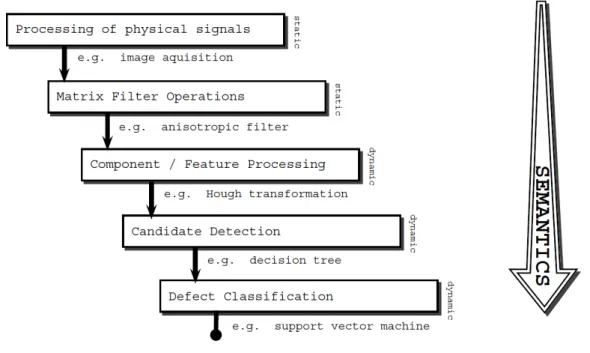
the use of high-performance computational hardware like GPUs or multi-core systems and the exploitation of parallelization potentials. The analysis of the whole processing pipeline (image acquisition, preprocessing, feature extraction, registration, defect detection and classification) with standard languages regarding performance is a resource- and time-intensive challenge. Figure 1 gives an example of such a image processing pipeline.

Figure 1. Typical image processing pipeline

While the performance of the image acquisition part mainly depends on the selected hardware and commu-nication interfaces, the performance of major parts of preprocessing and feature extraction can be computed in a well-predictable way, due to the fixed size of filter operations and the amount of data known in advance. Besides less computational intensive methods, e.g., thresholding, image arithmetic, etc., the application of more sophisticated preprocessing methods is indispensable, e.g., enhancement of faults with the anisotropic diffusion filter, however, it increases the execution time. Nevertheless, sophisticated preprocessing methods can reduce the complexity and hence the computational costs of high-level pattern recognition and classification methods. For example, at the beginning of the processing pipe, a typical low-level scenario uses local filter operations, acting, e.g., on 9x9 matrices, while afterwards global operations on the whole image data are applied, such as a registration with a reference model based on thousands of feature points. So far the processing steps are acting on a physical, appearance-based level which only depends on the image intensity values. Finally, defect candidates have to be identified, located and classified. This final high-level step heavily depends on parameters that are not coded within the image, e.g., the customer’s judgment whether some product quality aspects can be accepted or have to be rejected. The complexity of the classification step correlates with the quality of the

preprocessing on the one hand, i.e., the best possible enhancement of faults and elimination of noise, and with the complexity of the defect taxonomy on the other hand.

In this paper a comparison and benchmarking of different implementations of two major parts of the above introduced image processing pipeline is performed. One part is the investigation of the Perona-Malik Anisotropic Diffusion1_{) which has poor performance characteristics by default, and the other examined method is a}

classifi-cation by Support Vector Machines (SVMs).5 _{After a short overview of related work in Section 2, we introduce}

the functional array language SaC (Section 3). Then a detailed explanation of the anisotropic diffusion and

the the SVM (and the according parallelized versions) is given in Section 4. Afterwards, we compare theSaC

optimization strategies (with and/or without GPU support) against those of theopencv2.36 in Section 5.

Fi-nally, in Section 6 a comparison of the different implementations concerning programmability, understandability, productivity, maintainability is given.

2. RELATED WORK

The industry standard for programming NVidia GPUs is CUDA.7_{CUDA is a vendor-specific, architecture-specific}

and, hence, very low-level API. It allows the experienced programmer to adapt a program to the architectural peculiarities of GPU processing and to achieve high performance, if programming effort is not a big concern. However, software engineering on this level of abstraction is both tedious and cumbersome. If CUDA marks one end of the spectrum of GPU programming, thenSaC8 marks the other. SaC programs are

architecture-agnostic – it is solely up to the compiler and runtime system to make efficient use of GPUs where and when they are present.3 _{Our goal is to provide scientists whose areas of expertise lie elsewhere than in high-performance}

computing, with nearly the same program performance as if they had been written by a highly skilled computer programmer. Analysis of that trade-off between performance and productivity is the subject of this paper.

In between CUDA andSaC, a number of other approaches aim at facilitating GPU programming. OpenCL,9

originally proposed by Apple, is now promoted by AMD (the only major manufacturer of both multi-core CPUs and GPUs); in particular, AMDs upcoming Fusion architecture will soon combine both worlds on a single chip. OpenCL is only marginally more abstract than CUDA. Programmers defines computational kernels, which can be executed on different kinds of GPUs and even on multi-core CPUs. Instead of providing access to concrete architectural features, OpenCL abstracts them into a machine model that captures essential properties of today’s GPU-enhanced computing systems across individual manufacturers and models. Nonetheless, to obtain high performance, OpenCL programmers must concern themselves with a variety of machine-level details that lower their productivity.

OpenMP10_{has a track record of facilitating programming of symmetric shared memory systems (multi-core,}

multi-processor) through compiler directives. The OpenMPC11 _{project aims at generating CUDA code from}

eligible standard OpenMP directives. This approach is particularly attractive if application code is already equipped with OpenMP directives. Still, OpenMP is on a much lower abstraction level thanSaC. We want to

mention a recent proposal to extend OpenMP by clauses for the explicit placement of computations on the host or an a GPGPU.12

Last, but not least, HiCuda13 _{is another approach to programming NVidia GPUs. based on compiler}

direc-tives; it essentially imitates the OpenMP approach for symmetric multicores and proposes a tailor-made directive language for CUDA-enabled GPUs. Technically, HiCuda does simplify GPU programming, but it nonetheless exposes the same variety of architectural features as CUDA. Programmers need to make all relevant design decisions in application engineering, but can express them much more concisely than when using vanilla CUDA.

3. SINGLE ASSIGNMENT C

SaC is a purely functional programming language that, as far as possible, adopts a C-like notation to ease

transition of programmers with a background in imperative languages; the language core is a functional, side-effect-free, subset of ISO C; assignment sequences are treated as nested let-expressions, branches as conditional expressions and loops as tail-end recursive functions; details can be found in.8 _{Despite the radically different}

underlying execution model (context-free substitution of expressions vs. step-wise manipulation of global state), all language constructs adopted from C exhibit exactly the operational behaviour expected by C programmers. This equivalence allows programmers to choose their favourite style ofSaCcode; meanwhile, the compiler exploits

the benefits ofSaCś side-effect free semantics to provide advanced optimisations and automatic parallelisation.

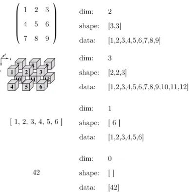
On top of this language kernel SaC provides genuine support for processing truly multidimensional (see

Figure 2) and truly stateless/functional arrays using a shape-generic style of programming. AnySaCexpression

evaluates to an array. Arrays may be passed between functions without restrictions. Array types include arrays of fixed shape, e.g.int[3,7], arrays of fixed rank, e.g. int[.,.], and arrays of any rank, e.g. int[*]. The

latter include scalars, which we, following APL, consider to be rank-0 arrays with an empty shape vector. For convenience and equivalence with C, we useint, rather than the equivalentint[], as a type notation for scalars.

The hierarchy of array types induces a subtype relationship, andSaCsupports function overloading with respect

to subtyping.

SaCprovides only a small set of built-in array operations. Essentially, there are primitives to retrieve data

⎛ ⎜⎜ ⎜⎜ ⎜ ⎝ 1 2 3 4 5 6 7 8 9 ⎞ ⎟⎟ ⎟⎟ ⎟ ⎠ dim: 2 shape: [3,3] data: [1,2,3,4,5,6,7,8,9] j k i 10 7 8 9 12 11 1 2 3 4 5 6 dim: 3 shape: [2,2,3] data: [1,2,3,4,5,6,7,8,9,10,11,12] [ 1, 2, 3, 4, 5, 6 ] dim: 1 shape: [ 6 ] data: [1,2,3,4,5,6] 42 dim: 0 shape: [ ] data: [42]

Figure 2. Truly multidimensional arrays inSaCand their representation by data vector, shape vector and rank scalar

...

... ... ... ...

int int[1] int[42] int[.] int[ ] int[.,.] int[1,1] int[3,7] rank: dynamic AUD Class: shape: static shape: dynamic AKD Class: rank: static shape: dynamic AKS Class: rank: static *

Figure 3. Three-level hierarchy of array types: arrays of unknown dimensionality (AUD), arrays of known dimensionality (AKD) and arrays of known shape (AKS)

A selection facility provides access to individual elements or entire subarrays using a familiar square bracket notation: array[idxvec].

All aggregate array operations are specified usingwith-loop expressions, aSaC-specific array comprehension: with {

(lower_bound <=idxvec <upper_bound): expr; }: genarray(shape,default)

They define a rectangular index set of arbitrary dimension. The identifieridxvecrepresents elements of this set,

similar to loop variables infor-loops. However, we deliberately do not define any order on these index sets.

Hence, awith-loop essentially specifies a FORALL loop nest. We call the specification of such an index set a generator and associate it with some potentially complex_SaCexpression. Thus, we create a mapping between

index vectors and values, in other words an array. As an example, consider thewith-loop

1 w i t h {

2 ( [ 0 , 0 ] <= i v < [ 3 , 5 ] ) : 4 2 ; 3 } : g e n a r r a y( [ 3 , 5 ] , 0)

that defines a3×5 matrix with all elements set to 42. The scope of the index vector,idxvec (here namediv)

is confined to the expression associated with the generator. The index vector can be used to access the current index location. For example, the with-loop

1 w i t h {

2 ( [ 0 ] <= i v < [ 5 ] ) : i v [ 0 ] ; 3 } : g e n a r r a y( [ 5 ] , 0)

computes the vector[0,1,2,3,4]. Note thativdenotes a 1-element vector rather than a scalar. Therefore, we

need to select the first (and only) element fromivto achieve the desired result. Actually, it is not the generator

that defines the shape of the resulting array, but the first expression following the keyword genarray. So far,

the two have always coincided, but for example

1 w i t h {

2 ( [ 1 ] <= i v < [ 4 ] ) : 4 2 ; 3 } : g e n a r r a y( [ 5 ] , 0)

computes the vector[0,42,42,42,0]. SaCstill creates a 5-element vector, but only the three inner elements

are defined as 42; all others are set to thedefault value, which is given by the second expression following the

key wordgenarray, in this case0. Since the default expression is not within the scope of a generator, it has no

access to the index. Hence, all array elements not covered by any generator are guaranteed to have the same value.

With-loops are not limited to a single generator. For example, thewith-loop

2 ( [ 1 ] <= i v < [ 4 ] ) : 1 ; 3 ( [ 3 ] <= i v < [ 5 ] ) : 2 ; 4 } : g e n a r r a y( [ 6 ] , 0)

defines the vector[0,1,1,2,2,0]. All elements of the resulting array still not covered by any of the generators

are initialised with the value of the default expression,0in the example. Whenever the index sets defined by the

various generators are not pairwise disjoint, the order of the generators matters: in the example the array’s value at index location [3], which is covered by both generators is set to 2 rather than to 1, i.e., the last generator

dominates.

SaCactually features several variants of with-loops. Let us assume we have named the array defined by the

previouswith-loopA. Then, themodarray-_with-loop

1 w i t h {

2 ( [ 0 ] <= i v < [ 3 ] ) : 3 ; 3 } : m o d a r r a y( A)

computes the vector[3,3,3,2,2,0]. More precisely, it computes a new array that has the same shape as the

existing array denoted by the expression following the key word modarray. The computation of those elements

covered by one or more generators follows exactly the same pattern as in the case of genarray-with-loops, but

the remaining elements are defined by the values of the corresponding elements in the referenced array rather than by a common default value. Furtherwith-loop variants support the definition of reduction operations and

strided index sets.

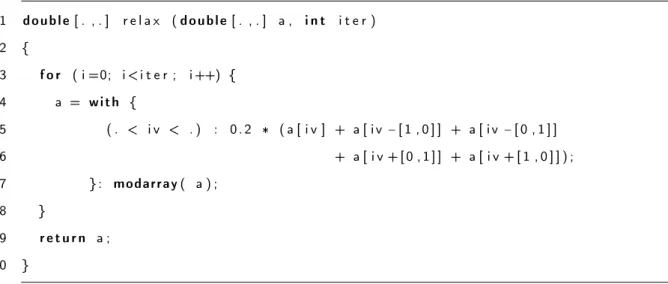
As a more complete example, consider the 2-dimensional, 5-point stencil relaxation shown in Figure 4. Here, a C-style FOR-loop implements iterative Jacobi-relaxation, while aSaCwith-loop array comprehension defines

a single relaxation step. The five nearest neighbour elements of the argument array aare selected using explicit

index computations. The dots in the generator refer to the least and the greatest index vector of the argument array a, respectively. In conjunction with the less-than relational operator, the dots form a convenient way to

define the set of all non-boundary indices of array a.

While with-loops can always be used to define application-specific array operations like the 5-point stencil relaxation in Figure 4, their primary purpose is to support the definition of rank- and shape-generic basic array processing building blocks, which we denote as the principle of abstraction. Those blocks, are then used to

1 d o u b l e[ . , . ] r e l a x (d o u b l e[ . , . ] a , i n t i t e r ) 2 { 3 f o r ( i =0; i <i t e r ; i ++) { 4 a = w i t h { 5 ( . < i v < . ) : 0 . 2 ∗ ( a [ i v ] + a [ iv −[ 1 , 0 ] ] + a [ iv −[ 0 , 1 ] ] 6 + a [ i v + [ 0 , 1 ] ] + a [ i v + [ 1 , 0 ] ] ) ; 7 } : m o d a r r a y( a ) ; 8 } 9 r e t u r n a ; 10 }

Figure 4. 2-dimensional 5-point stencil relaxation inSaC

1 d o u b l e[ ∗ ] s t e p (d o u b l e[ ∗ ] a ) 2 { 3 b = a ; 4 f o r ( d=0; d<dim( a ) ; i ++) { 5 b += r o t a t e ( d , −1 , a ) + r o t a t e ( d , 1 , a ) ; 6 } 7 r e t u r n b ∗ ( 1 . 0 / tod (2∗dim( a )+1)); 8 } 9 10 d o u b l e[ ∗ ] r e l a x (d o u b l e[ ∗ ] a , i n t i t e r ) 11 { 12 f o r ( i =0; i <i t e r ; i ++) { 13 a = s t e p ( a ) ; 14 } 15 r e t u r n a ; 16 }

langauges.

Figure 5 demonstrates howSaC code is engineered based on these principles. We first define a shape- and

rank-invariant version of nearest-neighbour relaxation that, as before, is based on a sequential FOR-loop to implement a series of relaxation steps. The function step uses another FOR-loop over the rank (number of

dimensions) of the argument array. In each dimension, we rotate the argument array by one element towards ascending indices and by one element towards descending indices and, eventually, add up all these arrays in an element-wise manner. Finally, we divide all elements of the resulting array by the number of additions, i.e. twice the rank of the argument array plus one (for the non-rotated argument array). The function todimplements

conversion from integer to floating point numbers. It is worthwhile to note that all functions used in the definition of step (e.g. rotation and element-wise array arithmetic) are not built-in primitives of theSaC language, but

are defined in theSaCstandard library, and are based onwith-loops.

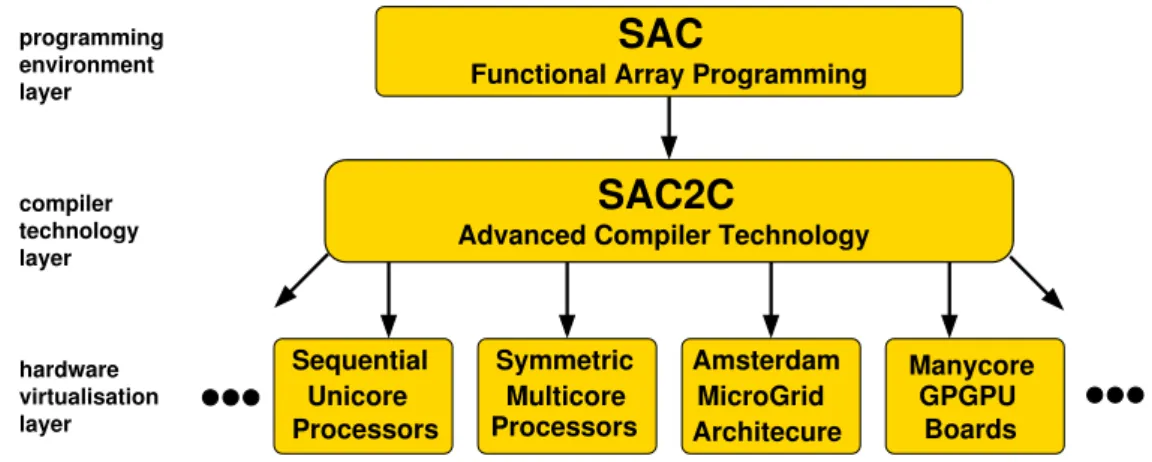
programming environment layer compiler technology layer layer hardware virtualisation Symmetric Processors Multicore Manycore GPGPU Boards MicroGrid Architecure Amsterdam Sequential Processors Unicore

Functional Array Programming

Advanced Compiler Technology

SAC

SAC2C

Figure 6. Architecture ofSaCcompilation infrastructure

As the various examples demonstrate,SaCcode is completely architecture-agnostic. The SaCcompilation

infrastructure sac2c exploits this fact to generate specific code for a variety of target hardware architectures

from the sameSaCsource code, thus achievinghardware virtualisation from a software engineering perspective.

Figure 6 illustrates this concept. Based on aggressively optimised sequential code14_{sac2cat the time of writing}

supports symmetric multicore multiprocessor systems15 _{, the MicroGrid chip multiprocessor architecture}4 _and

NVidia GPGPUs.16 _{Work is on-going to extend this list.}

4. APPLICATIONS

We now demonstrate how SaC combines high productivity in software engineering with high performance in

program execution, by means of two methods from the industrial inspection system introduced in Section 1. First, we present a brief theoretical introduction to the anisotropic diffusion filter of Perona-Malik,1 _{and to the}

decision function of the single class support vector machine.17 _{Then, we show our surprisingly simple and concise}

SaCimplementations of these applications.

4.1 Perona-Malik Anisotropic Diffusion

Essential factors for robust and reliable defect detection are the enhancement of defects, such as scratches or blowholes, and attenuation of environmental influences, e.g., irregular reflections, noise or dust. Defect enhancement is supported by the Perona-Malik anisotropic diffusion filter,1 _{whose principal characteristic is to}

reduce noise and concurrently enhance higher contrast regions.

The formal definition of the Perona-Malik anisotropic diffusion filter is defined by introducing D(., .)from

Equation (1) with the boundary condition in Equation (2), where D(., .) depends on the local derivative in

Equation (3) and Equation (4).

∂

∂tϕ=div(D∇ϕ), (1)

with boundary condition

ϕ(., .,0) =ϕ, (2)

whereD depends on the local derivatives. Perona-Malik propose two different derivates

D= 1 1+ (∥∇ϕ∥ K ) 2 (3) and D=exp−(∥∇ϕ∥/K)2 (4)

where Equation (3) acts as a smoothing filter that suppresses fine (noisy) structures, while Equation (4) strengthens high contrast edges. For an illustration, see Figure 7 to Figure 9, where we can see that only the connected wide regions are left, whereas noise structure is largely removed. The use of the deviation in Equa-tion (4) in Figure 9 shows us that beside the big deep scratch in the middle also fine, noisy, high contrast edges are left. Suppose that the parameters of the illustrated results in Figure 8 and Figure 9 are defined as follows: NITER is the number of iterations, which means how many times the filter should applied to the image, delta

Figure 7. stainless steel plate with noise surface and scratch

Figure 8. Application of Equation (3) on image of Figure 7; NITER=5; lambda=1/3; kappa=10;

Figure 9. Application of Equation (4) on image of Figure 7; NITER=5; lambda=1/3; kappa=10;

defines the stepsize of iteration and kappaKis the gradient modulus that controls the sensitivity to the edges.

The data-independent characteristic of the anisotropic diffusion filter allows an objective performance analysis of manually coded, as well as automaticallySaC generated, GPU code. We present benchmarking results in

section 5; subsection 4.2 outlines the implementation details of Perona-Malik anisotropic diffusion in Single Assignment C.

4.2 Implementation Single Assignment C versus Matlab

We show an abridgment of our SaC as well as Matlab implementation of the anisotropic diffusion filter. The

following comparison should give an impression of the similarity betweenSaCand Matlab syntax.

SaC

• . . .

• Line(3): apply the filter niter times • . . .

• Line(6-9): apply stencil operation • Line(12-15): calculate conduction • Line(17-20): assemble image • Line(23): return result

Matlab

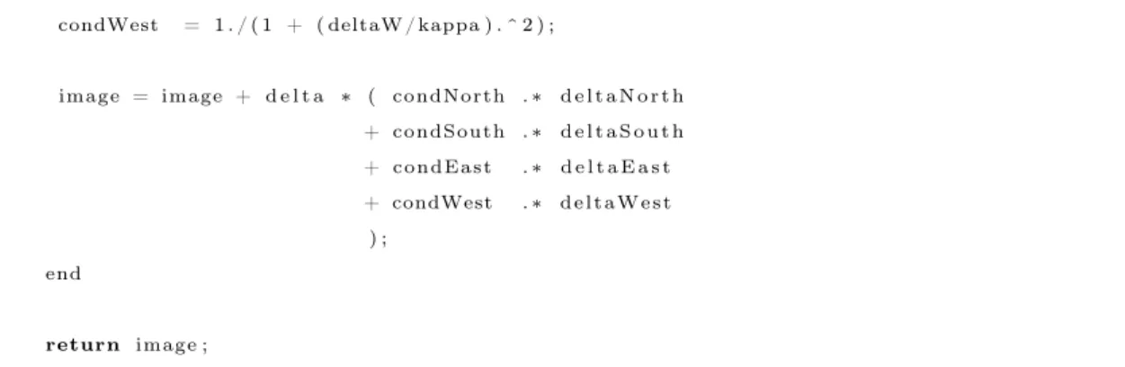
• Line(3): assign image dimension • Line(5): apply the filter niter times • Line(8-9): zero padding around image • Line(12-15): apply stencil operation • Line(18-21): calculate conduction • Line(23-27): assemble image • Line(30): return result

Beside of the assign of the image dimension (Matlab - Line(3)) and the zero padding around the image for stencil operation18 _{(Matlab - Line(8-9)) the differences of the code syntax are not significant.}

1 f l o a t[ . , . ] e x e c u t e A n i s o t r o p i c F i l t e r S A C (f l o a t[ . , . ] image , f l o a t kappa , f l o a t d e l t a , i n t n i t e r )

2 {

3 f o r ( i =0; i <n i t e r ; i ++)

4 {

5 /∗ s t e n c i l operation ∗/

6 deltaNorth = s h i f t ( 0 ,−1 , 0 f , image ) − image ;

7 d e l t a S o u t h = s h i f t ( 0 , 1 , 0 f , image ) − image ;

8 d e l t a E a s t = s h i f t ( 1 ,−1 , 0 f , image ) − image ;

9 deltaWest = s h i f t ( 1 , 1 , 0 f , image ) − image ;

10

11 /∗ Conduction ∗/

12 condNorth = 1 f / (1 f + pow ( deltaNorth / kappa , 2 f ) ) ; 13 condSouth = 1 f / (1 f + pow ( d e l t a S o u t h / kappa , 2 f ) ) ; 14 condEast = 1 f / (1 f + pow ( d e l t a E a s t / kappa , 2 f ) ) ; 15 condWest = 1 f / (1 f + pow ( deltaWest / kappa , 2 f ) ) ; 16

17 image += d e l t a ∗ ( condNorth ∗ deltaNorth 18 + condSouth ∗ d e l t a S o u t h 19 + condEast ∗ d e l t a E a s t 20 + condWest ∗ deltaWest ) 21 } 22 23 return image ; 24 }

Listing 2. Matlab implementation of Perona-Malik Anisotropic filter

1 f u n c t i o n image = executeAnisotropicFilterMATLAB ( image , n i t e r , kappa , d e l t a , o p t i o n ) 2 { 3 [ rows , c o l s ] = s i z e ( im ) ; 4 5 f o r i = 1 : n i t e r 6 7 % zero padding 8 d i f f l = z e r o s ( rows +2, c o l s +2); 9 d i f f l ( 2 : rows +1, 2 : c o l s +1) = image ; 10

11 % North , South , East and West d i f f e r e n c e s

12 deltaNorth = d i f f l ( 1 : rows , 2 : c o l s +1) − image ;

13 d e l t a S o u t h = d i f f l ( 3 : rows +2, 2 : c o l s +1) − image ;

14 d e l t a E a s t = d i f f l ( 2 : rows +1, 3 : c o l s +2) − image ;

15 deltaWest = d i f f l ( 2 : rows +1, 1 : c o l s ) − image ;

16

17 % Conduction

18 condNorth = 1 . / ( 1 + ( deltaN /kappa ) . ^ 2 ) ; 19 condSouth = 1 . / ( 1 + ( d e l t a S /kappa ) . ^ 2 ) ; 20 condEast = 1 . / ( 1 + ( deltaE /kappa ) . ^ 2 ) ;

21 condWest = 1 . / ( 1 + ( deltaW/kappa ) . ^ 2 ) ; 22

23 image = image + d e l t a ∗ ( condNorth . ∗ deltaNorth 24 + condSouth . ∗ d e l t a S o u t h 25 + condEast . ∗ d e l t a E a s t 26 + condWest . ∗ deltaWest 27 ) ; 28 end 29 30 return _{image ;}

4.3 Classification with One-Class Support Vector Machine

Support vector machines (SVM) are based on the concept of separating data of different classes by determining the optimal separating hyperplanes.19 _{The main idea behind support vector machines - and their distinctness}

to other learning algorithms - is the method ofstructural risk minimization. Instead of optimizing the training

error (which often leads to the problem of over-fitting), attention focuses on minimization of an estimate of the test error.5 Due to that underlying generalization,SVMs have become widely used learning methods which

provide state-of-the art solutions for various application areas, e.g. text categorization, texture analysis, and gene classification.

Typically, the SVM is a supervised learning algorithm working on two classes (binary classification, see also5_).

But for industrial quality inspection, where mostly large amounts of good samples are available and just a small fraction of possible defects are known, the application of an outlier-detection version has been proposed (one-class or single-class SVM, see17 _and20_{). The training of the one-class SVM (OC-SVM) relies only on one data class}

(positive samples) and tries to construct a hyperplane that separates the surface region containing data from the region containing no data. This is done by determining the hyperplane with maximal distance from the point of origin with all (or almost all) data points lying on the opposite side of the origin. For an illustration see figure 10.

Figure 10. One-Class SVM: Separation of data points and origin

and negative on the complement:

f(x) =sgn(∑ i

αik(xi,x) −ρ), (5)

where x is a new sample that needs to be classified. The kernel function k(., .) can be seen as similarity

measure between the new sample point and the support vectorsxi(a sub-set of the good samples from training,

describing the outer sphere of the data cluster). The parameterρ(decision boundary) and the non-zero weights αi (of the corresponding support vectorxi) are determined during the training phase.

For further details on the determination of the parameters and support vectors, and on possible kernel choices (polynomial, Gaussian radial basis function, etc.) see5 _and.21

For the following implementation inSaCand the benchmark tests (see Section 5), we use the Gaussian kernel

k(x,x′) =_e−γ∣∣x−x′∣∣2_,

withγ=_σ12, where σ>0 is the spread of the radial basis function, is used.

Often image processing applications are time-critical systems, e.g. in-line process control, where speed can be a limiting factor for usability. So the most essential part is the speed-up of the classification step, therefore a parallelization of the above mentioned decision function (see Equation 5) was considered.

4.4 Implementation in Single Assignment C

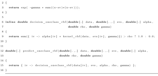
In this section, we implement the decision function of a single class support vector machine inSaC, see Listing 3.

In the Gaussian kernel function (kernel_rbf) the parameterxcontains the candidates to be classified, and the

parametersvcontains the trained support vectors. The second function, (decision_oneclass_rbfcomputes the

classification for one data point, wherealphais the weight of the according support vector. The 3rd (overloaded)

function (predict_oneclass_rbf), maps the 2nd function onto the whole data set, as demanded by equation 5.

Both overloaded instances of the decision_oneclass_rbffunction make use of_SaC’saxis control notation.22

Abstracting from some complexities of with-loops, this notation maps an index variable (in both casesiv) to

an index space that is derived from the shape of an array into which the index variable indices within the right hand side expression (e.g.datain the 2nd instance). That expression is evaluated for each legal index value and

the resulting values laminated to form a new array of the same shape as the one that is indexed into.

Listing 3.SaCimplementation of the decision function of support vector machine

2 {

3 return _{exp (} −gamma ∗ sum ( ( x−sv ) ∗ ( x−sv ) ) ) ;

4 } 5

6 i n l i n e double d e c i s i o n _ o n e c l a s s _ r b f (double[ . ] data , double[ . , . ] svs , double[ . ] alpha ,

7 double _{rho ,} double _gamma)

8 {

9 return sum({ i v −> alpha [ i v ] ∗ k e r n e l _ r b f ( data , s v s [ i v ] , gamma) } ) > rho ? 1 . 0 : 0 . 0 ;

10 } 11

12 double[ . ] p r e d i c t _ o n e c l a s s _ r b f (double[ . , . ] data , double[ . , . ] svs , double[ . ] alpha ,

13 double rho , double gamma)

14 {

15 return { i v −> d e c i s i o n _ o n e c l a s s _ r b f ( data [ i v ] , svs , alpha , rho , gamma) } ;

16 }

5. BENCHMARKING

Runtime benchmarking depends heavily on which hardware specification is used; also, the selection of hard-ware is problem specific. Hence, for our test scenario, we use two different hardhard-ware environments, i.e., a DELL Precision™_{690 and a SONY VAIO™PCG-81112M laptop. The DELL Precision}™_{690 has two separate}

Intel®_Xeon®_{5060 with 3.2GHz, giving 8 cores in total, and 2GB full buffered DDR2 memory, and a NVIDIA}

GeForce 8800 Ultra graphic card. The SONY VAIO™PCG-81112M laptop has an Intel®Core™i7-740QM Pro-cessor, 8GB RAM, and an NVIDIA GeForce GT 425M graphic card. The NVIDIA GeForce 8800 Ultra has 128 streaming processors with a core frequency of 612 MHZ, memory frequency of 1080MHz, 786MB memory and a memory bandwidth of 103.7 GB/sec where the NVIDIA GeForce GTX 425M has 96 streaming processors with a core frequency of 1120 MHZ, memory frequency of 800MHz, up to 1024 MB memory and a memory bandwidth of 25.6 GB/sec.

5.1 Benchmarking Anisotropic Diffusion

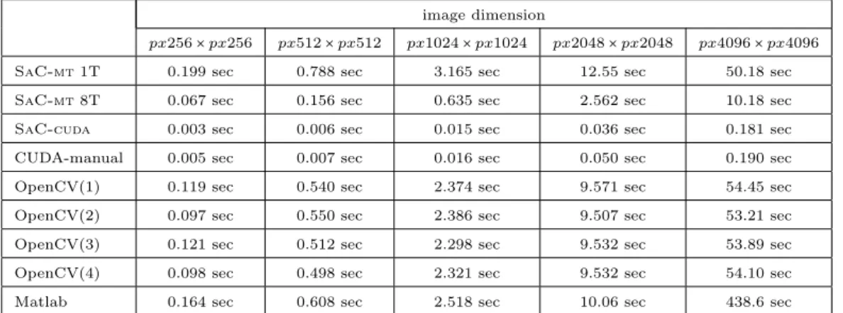
The dimension of the input data for the anisotropic filter ranges from 256×256 pixels to 4096×4096 pixels,

with pseudo-randomly generated 8-bit values between 0 and 255 since, in this example, only the dimension of the data affects execution time. Therefore, in Table 1 we present five different input sizes and propagate for each of them Equation (3) ten times. Furthermore, we implemented the filter inSaCwith auto generated

CPU-and CUDA-code; the CUDA version is manually optimized; the OpenCV2.3 framework is measured with CPU-and without GPU and Intel TBB support. Finally, a Matlab implementation is benchmarked as well.

Table 1 gives the benchmarking results achieved on the DELL Precision™_{690; Table 2 gives the same for}

sequential execution and SAC-MT 8T denotes automatic parallelization to 8 cores. For all non-trivial problem sizes, we observe a speedup of about 5. This reduction in runtime is realized with no more development effort, but solely recompilation of theSaC source code. In industrial practice, this substantial performance improvement

can be a time buffer for using more complex algorithms or giving a significant competitive advantage against other applications. Furthermore, the execution time of the auto-parallelizedSaC-cudacode compares favorably

with manually optimized CUDA-code. It can be generally observed that GPU and TBB support of the OpenCV implementation has, in this use case, no impact to the overall performance. In general, the runtime of the Matlab implementation is not as bad as expected but, for larger input sizes (e.g., 4096x4096), it runs out of memory, resulting in disastrous execution times.

image dimension

px256×px256 px512×px512 px1024×px1024 px2048×px2048 px4096×px4096

SaC-mt1T 0.199 sec 0.788 sec 3.165 sec 12.55 sec 50.18 sec SaC-mt8T 0.067 sec 0.156 sec 0.635 sec 2.562 sec 10.18 sec SaC-cuda 0.003 sec 0.006 sec 0.015 sec 0.036 sec 0.181 sec

CUDA-manual 0.005 sec 0.007 sec 0.016 sec 0.050 sec 0.190 sec OpenCV(1) 0.119 sec 0.540 sec 2.374 sec 9.571 sec 54.45 sec OpenCV(2) 0.097 sec 0.550 sec 2.386 sec 9.507 sec 53.21 sec OpenCV(3) 0.121 sec 0.512 sec 2.298 sec 9.532 sec 53.89 sec OpenCV(4) 0.098 sec 0.498 sec 2.321 sec 9.532 sec 54.10 sec Matlab 0.164 sec 0.608 sec 2.518 sec 10.06 sec 438.6 sec

Table 1. Runtime results of anisotropic filter benchmarked on a DELL Precision™_690,

SaC-mt 1T/8T =SaCon CPU executed with 1 and 8 threads,SaC-cuda=SaCimplementation, CUDA-manual = CUDA implementation, OpenCV(1) = OpenCV2.3v without CUDA and TBB support, OpenCV(2) = OpenCV2.3v with CUDA support, OpenCV(3) = OpenCV2.3v with TBB support, OpenCV(4) = OpenCV2.3v with CUDA and TBB support, Matlab = Matlab version 2011b.

But why do we not achieve a speedup of 8 with the CPU code? In fact, both experimental systems only feature 4 real cores which are twice hyperthreaded, but hyperthreading is not effective for this kind of workload. In this sense, the four-fold speedup is close to optimal. The functional programming paradigm results in a low memory usage of about 350 MB on average. However, if we need more performance for the application scenario, we have the possibility either to re-implement the whole algorithm with NVIDIAs CUDA framework or automatically generate executable GPU code with theSaC-cuda backend. A CUDA re-implementation definitely requires

higher development costs and programming know-how from experts, whereasSaC-cudaallows flexible time and

cost-efficient development.

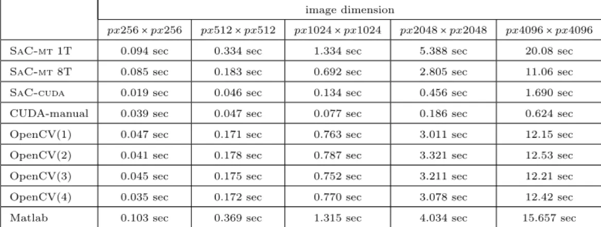
In Table 2 are the benchmarking results achieved on the SONY VAIO™PCG-81112M, where the general performance on CPU is slightly better than on DELL Precision™_{690. Although the SONY VAIO™PCG-81112M}

image dimension

px256×px256 px512×px512 px1024×px1024 px2048×px2048 px4096×px4096

SaC-mt1T 0.094 sec 0.334 sec 1.334 sec 5.388 sec 20.08 sec SaC-mt8T 0.085 sec 0.183 sec 0.692 sec 2.805 sec 11.06 sec SaC-cuda 0.019 sec 0.046 sec 0.134 sec 0.456 sec 1.690 sec

CUDA-manual 0.039 sec 0.047 sec 0.077 sec 0.186 sec 0.624 sec OpenCV(1) 0.047 sec 0.171 sec 0.763 sec 3.011 sec 12.15 sec OpenCV(2) 0.041 sec 0.178 sec 0.787 sec 3.321 sec 12.53 sec OpenCV(3) 0.045 sec 0.175 sec 0.752 sec 3.211 sec 12.21 sec OpenCV(4) 0.035 sec 0.172 sec 0.770 sec 3.078 sec 12.42 sec Matlab 0.103 sec 0.369 sec 1.315 sec 4.034 sec 15.657 sec

Table 2. Runtime results of anisotropic filter benchmarked on a SONY VAIO™PCG-81112M, SaC-mt 1T/8T = SaC on CPU executed with 1 and 8 threads, SaC-cuda = SaC implementation, CUDA-manual = CUDA implementa-tion, OpenCV(1) = OpenCV2.3v without CUDA and TBB support, OpenCV(2) = OpenCV2.3v with CUDA support, OpenCV(3) = OpenCV2.3v with TBB support, OpenCV(4) = OpenCV2.3v with CUDA and TBB support, Matlab = Matlab version 2011b.

has the newer graphic card, the benchmarks are significantly slower than on the DELL Precision™_{690, because}

of the lower hardware performance characteristic in the laptop.

5.2 Benchmarking One-Class SVM

We now present a comparison of the parallelized versions of the decision function (see Equation (5)). First, the

SaC-cudaimplementation, shown in Figure 3, is benchmarked. In addition toSaCruntime performance, we

present results of theGPUSVM23implementation and an OpenCV implementation compiled with GPU support,

as well as Intel TBB. The manually optimized implementation of the GPU-based OC-SVM Classifier is based on a third-party C-Support Vector Classification implementation called GPUSVM.23 For processing SVM data

in parallel on GPU-devices, the applied classification algorithm employs Map Reduce24 _{techniques proposed by}

Google as well as a GPU-vendor supplied Basic Linear Algebra Subroutines (CUBLAS). The developed

GPU-based OC-SVM classifier is able to read LIBSVM data format, hence, LIBSVM can be used for the training of the SVM models (and providing support vectors for it). Furthermore, all implementations can handle sparse matrices representation.

For the presented test results (shown in Table 3 and Table 4), some publicly available data sets were used from the LIBSVM data sets repository.25 _{Since this data repository does not contain data sets for OC-SVMs, we}

took binary sets and generated training data sets with a certain size (300 samples), consisting of data belonging only to one class. A simplified training with the standard settings of LIBSVM was performed, using the Gaussian RBF kernel withγ=1/n(wherenis the number of features of the input vectors) andν=0.5. For an explanation

data sets | # of data points | # of features

a1a | 30956 | 123 a9a | 32561 | 123 australian | 690 | 14 w8a | 49749 | 300

SaC-mt1T 9.484 sec 10.16 sec 0.479 sec 15.72 sec

SaC-mt8T 1.709 sec 1.885 sec 0.096 sec 2.850 sec

SaC-cuda 0.921 sec 0.951 sec 0.051 sec 1.356 sec

CUDA-manual 0.249 sec 0.253 sec 0.187 sec 0.295 sec

OpenCV(1) 6.241 sec 6.611 sec 0.055 sec 21.92 sec

OpenCV(2) 6.211 sec 6.598 sec 0.054 sec 21.76 sec

OpenCV(3) 1.410 sec 1.488 sec 0.017 sec 4.941 sec

OpenCV(4) 1.417 sec 1.494 sec 0.017 sec 4.939 sec

Table 3. Runtime results of decision function of single class support vector machine benchmarked on a DELL Precision™_690,

SaC-mt1T/8T =SaCon CPU executed with 1 and 8 threads, SaC-cuda=SaCimplementation, CUDA-manual = CUDA implementation, OpenCV(1) = OpenCV2.3v without CUDA and TBB support, OpenCV(2) = OpenCV2.3v with CUDA support, OpenCV(3) = OpenCV2.3v with TBB support, OpenCV(4) = OpenCV2.3v with CUDA and TBB support.

data sets | # of data points | # of features

a1a | 30956 | 123 a9a | 32561 | 123 australian | 690 | 14 w8a |49749 | 300

SaC-mt1T 6.379 sec 6.834 sec 0.248 sec 9.620 sec

SaC-mt8T 1.759 sec 1.865 sec 0.071 sec 3.097 sec

SaC-cuda 2.766 sec 2.949 sec 0.051 sec 3.882 sec

CUDA-manual 0.569 sec 0.613 sec 0.324 sec 0.794 sec

OpenCV(1) 3.066 sec 3.281 sec 0.037 sec 11.80 sec

OpenCV(2) 3.045 sec 3.265 sec 0.035 sec 11.83 sec

OpenCV(3) 1.284 sec 1.342 sec 0.014 sec 4.811 sec

OpenCV(4) 1.274 sec 1.322 sec 0.015 sec 4.812 sec

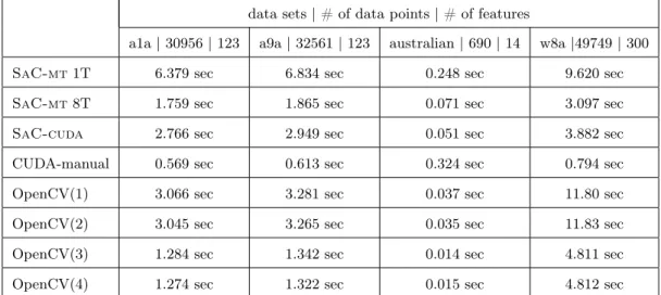
Table 4. Runtime results of decision function of single class support vector machine benchmarked on a SONY VAIO™PCG-81112M,SaC-mt1T/8T = SaCon CPU executed with 1 and 8 threads,SaC-cuda=SaC implementation, CUDA-manual = CUDA implementation, OpenCV(1) = OpenCV2.3v without CUDA and TBB support, OpenCV(2) = OpenCV2.3v with CUDA support, OpenCV(3) = OpenCV2.3v with TBB support, OpenCV(4) = OpenCV2.3v with CUDA and TBB support.

In general, we can observe for the one-class SVM use case in Table 3 and Table 4 that we achieve a speedup for all multi-core implementations (i.e.,SaC-mt 8T, OpenCV(3), OpenCV(4)) in opposite to single threaded

execution (i.e.,SaC-mt1T, OpenCV(1), OpenCV(2)). Especially for the test dataa1a,a9a, andaustralian the

on CPU showed the best runtime performance. This can be explained due to the high sparseness of the data matrix.

sparseness of data set features a1a 88.72% 88.69% a9a 88.72% 88.69% australian 20.04% 13.59% w8a 96.11% 94.58%

Table 5. Sparseness of the used data sets and features

In the OpenCV implementation the GPU support can be neglected because the used functions in the im-plementation provides no GPU support. The manual coded Cuda application can outperform the SaC-cuda

approximately 4.8 times, which mainly depends on the sparseness of the input matrices.

Concerning optimization strategies, we can say that OpenCV offers an optimized Streaming SIMD Exten-sions 2 (SSE2) code. SSE2 is a processor supplementary instruction set for modern 32-bit x86 and 64-bit x64 Single-Instruction, Multiple-Data (SIMD) architectures, where many of the basic arithmetic functions can run significantly faster. OpenCV also contains Intel®Threading Building Blocks (TBB)26_{support for several}

func-tions. TBB is a C++ template library which offers a complete threading mechanism on modern multi-core processors. The advantages of this library are easy and efficient handling ( application engineers do not need to be threading experts), scalable performance and a higher-level, task-based parallelism. In our example TBB is irrelevant as we do not use OpenCV functions that support this library. OpenCV applies the TBB only to OpenCV applications, e.g., haartraining, traincascade, and not to basic arithmetic/filter operations.

The optimization strategy ofSaC is different. One of the major design principles ofSaC is theWith-loop

construct, which supports the specification of shape-invariant array operations. All primitive array operations ofSaC can be defined as with-loops within a standard library rather than being implemented as part of the

compiler. The basic idea is to usewith-loops as a universal representation for array operations and to develop

a general transformation scheme that allows the concentration of individual with-loops into complex ones that exposes a more favorable computation to memory load/store ratio and reduces the need for synchronization and communication in parallel execution. Together, with-loop-folding, with-loop-fusion and with-loops27

stepwise transform any nesting of primitive array operations into a single loop construct that contains an element-wise specification of the resulting array. During the compilation process various conventional optimization techniques,28, 29_{such as function inlining, constant folding, constant propagation, loop unrolling, and dead code}

Posix™threads2, 30 or CUDA.3The net result is that application programmers can concentrate on the science of

their problem area, rather than being forced to become experts in parallel programming or GPU programming.

6. EXPERIENCES

This section evaluates various key values, i.e., programmability, understandability, productivity, maintainability, IDE support and CPU/GPU execution time, based on developer statements. Future development concerns make the choice of application implementation language a crucial decision. We investigated these issues by implementing our mentioned applications in C++/OpenCV, Matlab, CUDA and SaC taking care in software

engineering aspects during the whole application development life cycle. As a starting point, C programming skills are rated as neutral to allow comparison of language characteristics with other tools, languages and frameworks.

programmability understandability productivity maintainability IDE support execution time CPU GPU

C++/OpenCV ○ ○ ○ ○ ○ ○ ○

Matlab + ○ ○ + ++ −− ○

CUDA − − −− ○ + ○ ++

SAC ○ ○ ++ ++ −− ○ +

Table 6. Pros and cons of applied tools, languages and frameworks regarding various application development aspects

Researcher, developer and application engineers have different needs and expectations for languages and tools, hence each language has more or less a similarprogrammability andunderstandability, because of existing assets

and drawbacks in specific application fields, e.g., Matlab is a simple to use programming language, especially for rapid prototyping, but normally the developer has no knowledge about internal optimization strategies. For GPU development with CUDA, the developer needs special expertise in hardware architecture and parallelization techniques, and has to cope with a fast growing and changing technology. If the developer has good programming skills in C++/Matlab,SaCis easy to learn and provides the programming comfort of Matlab, e.g., no pointer

arithmetic. Furthermore,SaCprovides auto-parallelization and optimization over the whole application.

For rapid prototyping development, Matlab offers high productivity, our experience is that in several cases

a re-design/re-implementation, using a more efficient language/framework in terms of runtime, is needed. This is often intensive work because of the unknown optimization strategies within Matlab: results vary and are not comparable to the other languages. By using SaC it is possible to auto-generate code for the mentioned

platforms; this is especially useful if the performance criteria of a project have changed. SaC-code can fully

automatically be compiled to multicore CPUs, manycore GPUs and the MicroGrid chip multiprocessor architec-ture. This offers high flexibility during a project’s life cycle and it brings great advantages in maintainability.

re-compilation of the exact same source code. For the other languages, maintainability has basically a similar complexity.

A drawback of SaC is the lack of an integrated development environment (IDE support), which means

that debugging, code analysis, benchmarking, etc., can only be done via the command line, whereas the other tools, languages and frameworks offer consistently well-engineered tool support, e.g., on GPU the profiling and debugging can be done via external tools and integrated MS Visual Studio plugins.

Theexecution time on CPU and GPU is influenced by several factors, e.g., hardware environment,

paralleliza-tion and benchmarking strategies or concurrent producparalleliza-tion processes that primarily occur in industry. However, in general,SaCperformance on CPUs is as good as the performance of C if no optimization framework is used

(e.g., OpenCV, Intel-IPP, Intel-MKL, etc.). Typically, the highest performance can be achieved with manually written CUDA code (there are some exceptions) but in some cases SaC is able to surpass manually written

CUDA code due to whole program optimization and consistently optimized parallelization strategies, especially for array-based algorithms. Furthermore, the design of complex parallel algorithms inSaC is easier than with

CUDA; this often results in a bug-free and runtime-optimized application development.

7. CONCLUSION

In this paper, we showed the advantage of the functional array language Single Assignment C (SaC) in the field

of image processing, particularly for the anisotropic diffusion filter and for the decision function of a single class support vector machine. Such a sophisticated filter operation can enhance faults and eliminate noise in multi-iteration steps. This is computationally intensive, but indispensable to reduce the complexity, and consequently, the computational costs of high-level pattern recognition and classification methods. A single class support vector machine provides a robust and reliable classification for defect candidates which algorithmic characteristic allows a fine-grained parallelization and hence an optimal performance gain.

Due to industrial needs for balance between scalable and high-performance applications on the one hand and the demand for constant or lower development costs on the other hand, we conducted a benchmarking experiment in which we compared the development effort usingSaCand the common image library OpenCV2.3v.

In terms of language syntax, SaC is similar to Matlab because of the definition of various Matlab-like

operations. Furthermore, withSaC development time can be reduced by the well-known C/C++ semantics, yet

offering side-effect free semantics, most notably due to the absence of pointers and hardware virtualization. The hardware virtualization allows flexible and fast development on architectures corresponding to CPUs, GPUs or FPGAs using the same language and the same implementation. Moreover, on multi/many-core architectures, as

well as on GPUs,SaCwith auto-parallelization is often able to obtain higher performance than with the other

languages. Additionally, from the economic point of view, SaC provides us with an extremely good balance

between time of development and performance.

AlthoughSaCis well-suited for image processing as well as array based algorithms because of data-parallelism

and n-dimensional array support, it provides limited support for development and debugging tools. This will be changed in the future by an intensive enhancement ofSaCand community building.

ACKNOWLEDGMENTS

Our work is funded by the EU FP7-projectADVANCEand the FFG-basis program.

REFERENCES

[1] Perona, P. and Malik, J., “Scale-space and edge detection using anisotropic diffusion,” IEEE Transactions on Pattern Analysis and Machine Intelligence12, 629–639 (1990).

[2] Grelck, C., “Shared memory multiprocessor support for functional array processing in SAC,” Journal of Functional Programming15(3), 353–401 (2005).

[3] Guo, J., Thiyagalingam, J., and Scholz, S.-B., “Towards Compiling SaC to CUDA,” in [10th Symposium on Trends in Functional Programming (TFP’09)], Horváth, Z. and Viktória Zsók, eds., 33–49, Intellect (2009).

[4] Grelck, C., Herhut, S., Jesshope, C., Joslin, C., Lankamp, M., Scholz, S.-B., and Shafarenko, A., “Compiling the Functional Data-Parallel Language SaCfor Microgrids of Self-Adaptive Virtual Processors,” in [14th Workshop on Compilers for Parallel Computing (CPC’09), IBM Research Center, Zürich, Switzerland],

(2009).

[5] Schölkopf, B. and Smola, A. J., [Learning with Kernels: Support Vector Machines, Regularization, Opti-mization, and Beyond (Adaptive Computation and Machine Learning)], The MIT Press (2001).

[6] Bradski, G., “The OpenCV Library,” Dr. Dobb’s Journal of Software Tools(2000).

[7] David B. Kirk, Wen-mei W. Hwu, [Programming Massively Parallel Processors: A Hands-on Approach],

Morgan Kaufmann (2010).

[8] Grelck, C. and Scholz, S.-B., “SAC: A functional array language for efficient multithreaded execution,”

International Journal of Parallel Programming34(4), 383–427 (2006).

[9] Tsuchiyama, R., Nakamura, T., Iizuka, T., Asahara, A., Miki, S., and Tagawa, S., [The OpenCL Program-ming Book], Fixstars (2010).

[10] Chapman, B., Jost, G., and van der Pas, R., [Using OpenMP: Portable Shared Memory Parallel Program-ming], MIT Press (2007).

[11] Lee, S. and Eigenmann, R., “OpenMPC: Extended OpenMP Programming and Tuning for GPUs,” in [ACM/IEEE International Conference for High Performance Computing, Networking, Storage and Analysis (SC’10), New Orleans, USA], IEEE (2010).

[12] Ayguade, E., Badia, R., Cabrera, D., Duran, A., Gonzalez, M., et al., “A proposal to extend the openmp tasking model for heterogeneous architectures,” in [Evolving OpenMP in an Age of Extreme Parallelism, 5th International Workshop on OpenMP (IWOMP’09), Dresden, Germany], Mueller, M., de Supinski, B., and

Chapman, B., eds.,Lecture Notes in Computer Science 5568, 154–167, Springer-Verlag (2009).

[13] Han, T. and Abdelrahman, T., “hiCUDA: A High-level Directive-based Language for GPU Programming,” in [2nd Workshop on General Purpose Processing on Graphics Processing Units (GPGPU-2), Washington, USA], 52–61, ACM (2009).

[14] Grelck, C. and Scholz, S.-B., “Merging compositions of array skeletons in SAC,” in [Parallel Computing: Current and Future Issues of High-End Computing, International Conference ParCo 2005, Malaga, Spain],

Joubert, G., Nagel, W., Peters, F., Plata, O., Tirado, P., and Zapata, E., eds., NIC Series33, 859–866,

John von Neumann Institute for Computing, Jülich, Germany (2006). [ISBN 3-00-017352-8].

[15] Grelck, C. and Scholz, S.-B., “Sac: a functional array language for efficient multi-threaded execution,” Int. J. Parallel Program.34, 383–427 (August 2006).

[16] Guo, J., Thiyagalingam, J., and Scholz, S.-B., “Breaking the gpu programming barrier with the auto-parallelising sac compiler,” in [Annual Symposium on Principles of Programming Languages, 6th Workshop on Declarative Aspects of Multicore Programming (DAMP’11), Austin, Texas, USA], 15–24, ACM Press,

New York City, New York, USA (2011).

[17] Schölkopf, B., Williamson, R., Smola, A., Shawe-Taylor, J., and Platt, J., “Support vector method for novelty detection,” Advances in Neural Information Processing Systems12 (2000).

[18] Patten, C. J., James, H., Hawick, K., and Brown, A. L., “Stencil methods on distributed high performance computers,” tech. rep. (1997).

[19] Vapnik, V., [Statistical Learning Theory], Wiley, New York (1998). forthcoming.

[20] Schölkopf, B., Platt, J. C., Shawe-Taylor, J. C., Smola, A. J., and Williamson, R. C., “Estimating the support of a high-dimensional distribution,” Neural Comput.13, 1443–1471 (July 2001).

[21] Cristianini, N. and Shawe-Taylor, J., [Support Vector Machines and Other Kernel-based Learning Methods],

Cambridge University Press (2000).

[22] Grelck, C. and Scholz, S.-B., “Axis Control in SAC,” in [Implementation of Functional Languages, 14th International Workshop (IFL’02), Madrid, Spain, Revised Selected Papers], Peña, R. and Arts, T., eds., Lecture Notes in Computer Science 2670, 182–198, Springer-Verlag, Berlin, Germany (2003).

[23] Catanzaro, B. C., Sundaram, N., and Keutzer, K., “Fast support vector machine training and classification on graphics processors,” Tech. Rep. UCB/EECS-2008-11, EECS Department, University of California, Berkeley (Feb 2008).

[24] Dean, J. and Ghemawat, S., “Mapreduce: simplified data processing on large clusters,”Commun. ACM51,

107–113 (January 2008).

[25] “LIBSVM Data: Classification, Regression, and Multi-label.” http://www.csie.ntu.edu.tw/~cjlin/ libsvmtools/datasets/.

[26] Reinders, J., [Intel threading building blocks], O’Reilly & Associates, Inc., Sebastopol, CA, USA, first ed.

(2007).

[27] Grelck, C. and Scholz, S.-B., “Merging compositions of array skeletons in SAC,” Journal of Parallel Com-puting 32(7+8), 507–522 (2006).

[28] Kennedy, K. and Allen, J. R., [Optimizing compilers for modern architectures: a dependence-based approach],

Morgan Kaufmann Publishers Inc., San Francisco, CA, USA (2002).

[29] Grelck, C. and Scholz, S., “SaC – from High-Level Programming with Arrays to Efficient Parallel Execution,”

Parallel Processing Letters13(3), 401–412 (2003).

[30] “IEEE Standard for Information Technology - Portable Operating System Interface (POSIX). Base Defini-tions,” IEEE Std 1003.1, 2004 Edition. The Open Group Technical Standard Base Specifications, Issue 6. Includes IEEE Std 1003.1-2001, IEEE Std 1003.1-2001/Cor 1-2002 and IEEE Std 1003.1-2001/Cor 2-2004. Base, 0 1 (2004).