This file contains only one chapter of the book. For a free download of the complete book in pdf format, please visitwww.aimms.comor order your hard-copy atwww.lulu.com/aimms.
Copyright c1993–2012 by Paragon Decision Technology B.V. All rights reserved. Paragon Decision Technology B.V.
Schipholweg 1 2034 LS Haarlem The Netherlands Tel.: +31 23 5511512 Fax: +31 23 5511517
Paragon Decision Technology Inc. 500 108th Avenue NE Ste. # 1085 Bellevue, WA 98004 USA Tel.: +1 425 458 4024 Fax: +1 425 458 4025 Paragon Decision Technology Pte. Ltd.
55 Market Street #10-00 Singapore 048941 Tel.: +65 6521 2827 Fax: +65 6521 3001
Paragon Decision Technology Shanghai Representative Office Middle Huaihai Road 333 Shuion Plaza, Room 1206 Shanghai China Tel.: +86 21 51160733 Fax: +86 21 5116 0555 Email: [email protected] WWW:www.aimms.com
Aimmsis a registered trademark of Paragon Decision Technology B.V.IBM ILOG CPLEXandCPLEXis a registered trademark of IBM Corporation.GUROBIis a registered trademark of Gurobi Optimization, Inc. KNITROis a registered trademark of Ziena Optimization, Inc. XPRESS-MPis a registered trademark of FICO Fair Isaac Corporation. Mosekis a registered trademark of Mosek ApS.WindowsandExcelare registered trademarks of Microsoft Corporation. TEX, LATEX, andAMS-LATEX are trademarks of the American Mathematical Society.Lucidais a registered trademark of Bigelow & Holmes Inc.Acrobatis a registered trademark of Adobe Systems Inc. Other brands and their products are trademarks of their respective holders.
Information in this document is subject to change without notice and does not represent a commitment on the part of Paragon Decision Technology B.V. The software described in this document is furnished under a license agreement and may only be used and copied in accordance with the terms of the agreement. The documentation may not, in whole or in part, be copied, photocopied, reproduced, translated, or reduced to any electronic medium or machine-readable form without prior consent, in writing, from Paragon Decision Technology B.V.
Paragon Decision Technology B.V. makes no representation or warranty with respect to the adequacy of this documentation or the programs which it describes for any particular purpose or with respect to its adequacy to produce any particular result. In no event shall Paragon Decision Technology B.V., its employees, its contractors or the authors of this documentation be liable for special, direct, indirect or consequential damages, losses, costs, charges, claims, demands, or claims for lost profits, fees or expenses of any nature or kind.
In addition to the foregoing, users should recognize that all complex software systems and their doc-umentation contain errors and omissions. The authors, Paragon Decision Technology B.V. and its em-ployees, and its contractors shall not be responsible under any circumstances for providing information or corrections to errors and omissions discovered at any time in this book or the software it describes, whether or not they are aware of the errors or omissions. The authors, Paragon Decision Technology B.V. and its employees, and its contractors do not recommend the use of the software described in this book for applications in which errors or omissions could threaten life, injury or significant loss. This documentation was typeset by Paragon Decision Technology B.V. using LATEX and theLucidafont family.
General Optimization Modeling
Tricks
Chapter
6
Linear Programming Tricks
This chapter
This chapter explains severaltricksthat help to transform some models with special, for instance nonlinear, features into conventional linear programming models. Since the fastest and most powerful solution methods are those for linear programming models, it is often advisable to use this format instead of solving a nonlinear or integer programming model where possible.
References
The linear programming tricks in this chapter are not discussed in any partic-ular reference, but are scattered throughout the literature. Several tricks can be found in [Wi90]. Other tricks are referenced directly.
Statement of a linear program
Throughout this chapter the following general statement of a linear program-ming model is used:
Minimize: X j∈J cjxj Subject to: X j∈J aijxj≷bi ∀i∈I xj≥0 ∀j∈J
In this statement, the cj’s are referred to ascost coefficients, theaij’s are re-ferred to asconstraint coefficients, and thebi’s are referred to asrequirements. The symbol “≷” denotes any of “≤” , “=”, or “≥” constraints. A maximiza-tion model can always be written as a minimizamaximiza-tion model by multiplying the objective by (−1) and minimizing it.
6.1
Absolute values
The model
Consider the following model statement:
Minimize: X j∈J cj|xj| cj>0 Subject to: X j∈J aijxj≷bi ∀i∈I xj free
Instead of the standard cost function, a weighted sum of the absolute values of the variables is to be minimized. To begin with, a method to remove these absolute values is explained, and then an application of such a model is given.
Handling absolute values. . .
The presence of absolute values in the objective function means it is not possi-ble to directly apply linear programming. The absolute values can be avoided by replacing eachxjand|xj|as follows.
xj = x+j −xj−
|xj| = x+j +xj− x+
j, x−j ≥0
The linear program of the previous paragraph can then be rewritten as follows.
Minimize: X j∈J cj(x+j +xj−) cj>0 Subject to: X j∈J aij(xj+−xj−)≷bi ∀i∈I xj+, xj−≥0 ∀j∈J . . .correctly
The optimal solutions of both linear programs are the same if, for eachj, at least one of the valuesx+
j andx−j is zero. In that case,xj=x+j whenxj ≥0, and xj = −x−j whenxj ≤0. Assume for a moment that the optimal values ofx+j and x−j are both positive for a particularj, and letδ = min{x+j, x−j}. Subtracting δ > 0 from both xj+ and xj− leaves the value ofxj = xj+−xj− unchanged, but reduces the value of|xj| =x+j+xj−by 2δ. This contradicts the optimality assumption, because the objective function value can be reduced by 2δcj.
Application: curve fitting
Sometimesxjrepresents adeviationbetween the left- and the right-hand side of a constraint, such as in regression. Regression is a well-known statistical method of fitting a curve through observed data. One speaks oflinear regres-sionwhen a straight line is fitted.
Example
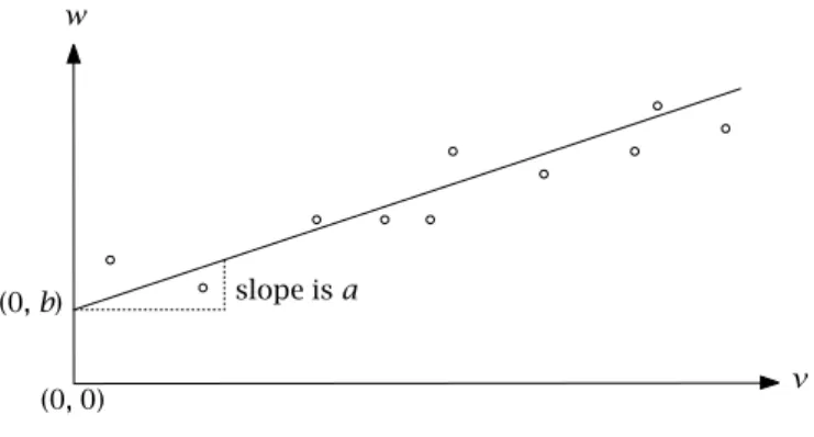
Consider fitting a straight line through the points(vj, wj)in Figure6.1. The coefficientsaandbof the straight linew=av+bare to be determined. The coefficientais theslopeof the line, andbis theinterceptwith thew-axis. In general, these coefficients can be determined using a model of the following form:
Minimize: f (z)
Subject to:
Chapter 6. Linear Programming Tricks 65 v w (0,b) (0, 0) slope isa
Figure 6.1: Linear regression
In this modelzjdenotes the difference between the value ofavj+bproposed by the linear expression and the observed value,wj. In other words,zj is the
erroror deviation in thewdirection. Note that in this casea,b, andzjare the decision variables, whereasvj andwj are data. A functionf (z)of the error variables must be minimized. There are different options for the objective functionf (z).
Different objectives in curve fitting Least-squares estimationis an often used technique that fits a line such that
the sum of the squared errors is minimized. The formula for the objective function is:
f (z)=X
j∈J z2
j
It is apparent that quadratic programming must be used for least squares es-timation since the objective is quadratic.
Least absolute deviations estimationis an alternative technique that minimizes the sum of the absolute errors. The objective function takes the form:
f (z)= X
j∈J
|zj|
When the data contains a few extreme observations,wj, this objective is ap-propriate, because it is less influenced by extreme outliers than is least-squares estimation.
Least maximum deviation estimationis a third technique that minimizes the maximum error. This has an objective of the form:
f (z)=max j∈J |zj|
This form can also be translated into a linear programming model, as ex-plained in the next section.
6.2
A minimax objective
The model
Consider the model
Minimize: max k∈K X j∈J ckjxj Subject to: X j∈J aijxj≷bi ∀i∈I xj≥0 ∀j∈J
Such an objective, which requires a maximum to be minimized, is known as a
minimax objective. For example, whenK = {1,2,3} andJ = {1,2}, then the objective is:
Minimize: max{c11x1+c12x2c21x1+c22x2c31x1+c32x2}
An example of such a problem is in least maximum deviation regression, ex-plained in the previous section.
Transforming a minimax objective
The minimax objective can be transformed by including an additional decision variablez, which represents the maximum costs:
z=max k∈K
X j∈J
ckjxj
In order to establish this relationship, the following extra constraints must be imposed:
X j∈J
ckjxj≤z ∀k∈K
Now whenzis minimized, these constraints ensure thatzwill be greater than, or equal to, Pj∈Jckjxj for all k. At the same time, the optimal value of z will be no greater thanthe maximum of all Pj∈Jckjxj because z has been minimized. Therefore the optimal value of z will be both as small as possible and exactly equal to the maximum cost overK.
The equivalent linear program Minimize: z Subject to: X j∈J aijxj≷bi ∀i∈I X j∈J ckjxj≤z ∀k∈K xj≥0 ∀j∈J
The problem of maximizing a minimum (a maximinobjective) can be trans-formed in a similar fashion.
Chapter 6. Linear Programming Tricks 67
6.3
A fractional objective
The model
Consider the following model:
Minimize: X j∈J cjxj+α , X j∈J djxj+β Subject to: X j∈J aijxj≷bi ∀i∈I xj≥0 ∀j∈J
In this problem the objective is the ratio of two linear terms. It is assumed that the denominator (the expressionPj∈Jdjxj+β) is either positive or neg-ative over the entire feasible set ofxj. The constraints are linear, so that a linear program will be obtained if the objective can be transformed to a linear function. Such problems typically arise in financial planning models. Possible objectives include the rate of return, turnover ratios, accounting ratios and productivity ratios.
Transforming a fractional objective
The following method for transforming the above model into a regular linear programming model is from Charnes and Cooper ([Ch62]). The main trick is to introduce variablesyjandtwhich satisfy:yj=txj. In the explanation below, it is assumed that the value of the denominator is positive. If it is negative, the directions in the inequalities must be reversed.
1. Rewrite the objective function in terms oft, where
t=1/(X j∈J
djxj+β)
and add this equality and the constraintt >0 to the model. This gives:
Minimize: X j∈J cjxjt+αt Subject to: X j∈J aijxj≷bi ∀i∈I X j∈J djxjt+βt=1 t >0 xj≥0 ∀j∈J
2. Multiply both sides of the original constraints byt, (t >0), and rewrite the model in terms ofyjandt, whereyj=xjt. This yields the model:
Minimize: X j∈J cjyj+αt Subject to: X j∈J aijyj≷bit ∀i∈I X j∈J djyj+βt=1 t >0 yj≥0 ∀j∈J
3. Finally, temporarily allow tto be≥0 instead of t >0 in order to get a linear programming model. This linear programming model is equivalent to the fractional objective model stated above, provided t > 0 at the optimal solution. The values of the variablesxj in the optimal solution of the fractional objective model are obtained by dividing the optimalyj by the optimalt.
6.4
A range constraint
The model
Consider the following model:
Minimize: X j∈J cjxj Subject to: di≤ X j∈J aijxj≤ei ∀i∈I xj≥0 ∀j∈J
When one of the constraints has both an upper and lower bound, it is called a range constraint. Such a constraint occurs, for instance, when a minimum amount of a nutrient is required in a blend and, at the same time, there is a limited amount available.
Handling a range constraint
The most obvious way to model such a range constraint is to replace it by two constraints: X j∈J aijxj≥di and X j∈J aijxj≤ei ∀i∈I
However, as each constraint is now stated twice, both must be modified when changes occur. A more elegant way is to introduce extra variables. By intro-ducing new variablesuione can rewrite the constraints as follows:
ui+ X j∈J
Chapter 6. Linear Programming Tricks 69
The following bound is then imposed onui:
0≤ui≤ei−di ∀i∈I
It is clear thatui=0 results in X j∈J aijxj=ei whileui=ei−diresults in X j∈J aijxj=di The equivalent linear program
A summary of the formulation is:
Minimize: X j∈J cjxj Subject to: ui+ X j∈J aijxj=ei ∀i∈I xj≥0 ∀j∈J 0≤ui≤ei−di ∀i∈I
6.5
A constraint with unknown-but-bounded coefficients
This section
This section considers the situation in which the coefficients of a linear in-equality constraint are unknown-but-bounded. Such an inin-equality in terms of uncertainty intervals is not a deterministic linear programming constraint. Any particular selection of values for these uncertain coefficients results in an unreliable formulation. In this section it will be shown how to transform the original nondeterministic inequality into a set of deterministic linear program-ming constraints.
Unknown-but-bounded coefficients
Consider the constraint with unknown-but-bounded coefficients ˜aj X
j∈J ˜
ajxj≤b
where ˜aj assumes an unknown value in the interval [Lj, Uj], b is the fixed right-hand side, andxjrefers to the solution variables to be determined. With-out loss of generality, the corresponding bounded uncertainty intervals can be written as[aj−∆j, aj+∆j], whereaj is the midpoint of[Lj, Uj].
Midpoints can be unreliable
Replacing the unknown coefficients by their midpoint results in a deterministic linear programming constraint that is not necessarily a reliable representation of the original nondeterministic inequality. Consider the simple linear pro-gram
Maximize: x
Subject to:
˜
ax≤8
with the uncertainty interval ˜a ∈[1,3]. Using the midpointa= 2 gives the optimal solutionx=4. However, if the true value of ˜ahad been 3 instead of the midpoint value 2, then forx=4 the constraint would have been violated by 50%.
Worst-case analysis
Consider a set of arbitrary but fixedxjvalues. The requirement that the con-straint with unknown-but-bounded coefficients must hold for the unknown values of ˜aj is certainly satisfied when the constraint holds for all possible values of ˜aj in the interval [aj−∆j, aj+∆j]. In that case it suffices to con-sider only those values of ˜aj for which the term ˜ajxj attains its maximum value. Note that this situation occurs when ˜ajis at one of its bounds. The sign ofxj determines which bound needs to be selected.
˜
ajxj≤ajxj+∆jxj ∀xj≥0 ˜
ajxj≤ajxj−∆jxj ∀xj≤0
Note that both inequalities can be combined into a single inequality in terms of|xj|. ˜ ajxj≤ajxj+∆j|xj| ∀xj An absolute value formulation
As a result of the above worst-case analysis, solutions to the previous formula-tion of the original constraint with unknown-but-bounded coefficients ˜aj can now be guaranteed by writing the following inequality without reference to ˜aj.
X j∈J ajxj+ X j∈J ∆j|xj| ≤b A tolerance. . .
In the above absolute value formulation it is usually too conservative to require that the original deterministic value of b cannot be loosened. Typically, a toleranceδ >0 is introduced to allow solutionsxjto violate the original right-hand sidebby an amount of at mostδmax(1,|b|).
Chapter 6. Linear Programming Tricks 71
. . .relaxes the right-hand side
The term max(1,|b|)guarantees a positive increment of at leastδ, even in case the right-hand sidebis equal to zero. This modified right-hand side leads to the followingδ-toleranceformulation where a solutionxjis feasible whenever it satisfies the following inequality.
X j∈J ajxj+ X j∈J ∆j|xj| ≤b+δmax(1,|b|) The final formulation
This δ-tolerance formulation can be rewritten as a deterministic linear pro-gramming constraint by replacing the |xj|terms with nonnegative variables yj, and requiring that−yj≤xj≤yj. It is straightforward to verify that these last two inequalities imply thatyj ≥ |xj|. These two terms are likely to be equal when the underlying inequality becomes binding for optimalxj values in a linear program. The final result is the following set of deterministic lin-ear programming constraints, which captures the uncertainty reflected in the original constraint with unknown-but-bounded coefficients as presented at the beginning of this section.
X j∈J ajxj+ X j∈J ∆jyj≤b+δmax(1,|b|) −yj≤xj≤yj yj≥0
6.6
A probabilistic constraint
This sectionThis section considers the situation that occurs when the right-hand side of a linear constraint is a random variable. As will be shown, such a constraint can be rewritten as a purely deterministic constraint. Results pertaining to proba-bilistic constraints (also referred to as chance-constraints) were first published by Charnes and Cooper ([Ch59]).
Stochastic right-hand side
Consider the following linear constraint
X j∈J
ajxj≤B
where J = {1,2, . . . , n} and B is a random variable. A solution xj, j ∈ J, is feasible when the constraint is satisfied for all possible values ofB.
Acceptable values only
For open-ended distributions the right-hand sideBcan take on any value be-tween−∞and +∞, which means that there cannot be a feasible solution. If the distribution is not open-ended, suppose for instance thatBmin≤B≤Bmax,
practical applications, it does not make sense for the above constraint to hold for all values ofB.
A probabilistic constraint
Specifying that the constraint Pj∈Jajxj ≤ B must hold for all values of B is equivalent to stating that this constraint must hold with probability 1. In practical applications it is natural to allow for a small margin of failure. Such failure can be reflected by replacing the above constraint by an inequality of the form Pr X j∈J ajxj≤B ≥1−α
which is called a linear probabilistic constraint or alinear chance-constraint. Here Pr denotes the phrase ”Probability of”, andαis a specified constant frac-tion (∈[0,1]), typically denoting the maximum error that is allowed.
Deterministic equivalent
Consider the density function fB and a particular value ofα as displayed in Figure6.2.
ˆ
B
B-axis 1−α
Figure 6.2: A density functionfB
A solution xj, j ∈ J, is considered feasible for the above probabilistic con-straint if and only if the term Pj∈Jajxj takes a value beneath point ˆB. In this case a fraction(1−α)or more of all values ofB will be larger than the value of the termPj∈Jajxj. For this reason ˆBis called thecritical value. The probabilistic constraint of the previous paragraph has therefore the following deterministic equivalent: X j∈J ajxj≤Bˆ Computation of critical value
The critical value ˆBcan be determined by integrating the density function from
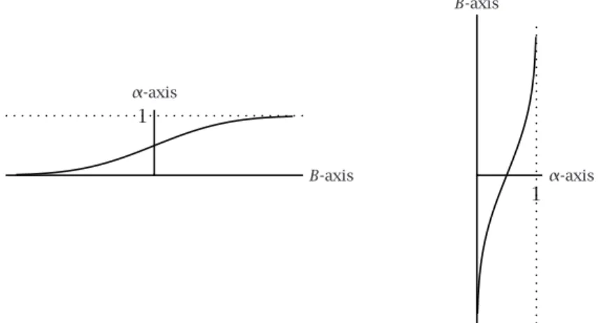
−∞until a point where the area underneath the curve becomes equal toα. This point is then the value of ˆB. Note that the determination of ˆBas described in this paragraph is equivalent to using the inverse cumulative distribution func-tion offB evaluated atα. From probability theory, the cumulative distribution
Chapter 6. Linear Programming Tricks 73
function FB is defined by FB(x) = Pr[B ≤ x]. The value of FB is the cor-responding area underneath the curve (probability). Its inverse specifies for each particular level of probability, the point ˆB for which the integral equals the probability level. The cumulative distribution function FB and its inverse are illustrated in Figure6.3.
B-axis α-axis 1 1 α-axis B-axis
Figure 6.3: Cumulative distribution functionF and its inverse.
Use
Aimms-supplied function
As the previous paragraph indicated, the critical ˆBcan be determined through the inverse of the cumulative distribution function. Aimmssupplies this func-tion for a large number of distribufunc-tions. For instance, when the underlying distribution is normal with mean 0 and standard deviation 1, then the value of ˆ
Bcan be found as follows:
ˆ
B=InverseCumulativeDistribution( Normal(0,1) ,α)
Example
Consider the constraint Pjajxj ≤ B with a stochastic right-hand side. Let B=N(0,1)andα=0.05. Then the value of ˆBbased on the inverse cumulative distribution is -1.645. By requiring thatPjajxj≤ −1.645, you make sure that the solutionxj is feasible for 95% of all instances of the random variableB.
Overview of probabilistic constraints
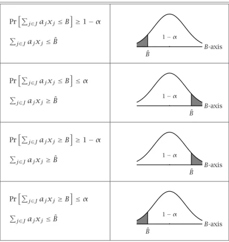
The following figure presents a graphical overview of the four linear proba-bilistic constraints with stochastic right-hand sides, together with their deter-ministic equivalent. The shaded areas correspond to the feasible region of
P
PrhPj∈Jajxj≤B i ≥1−α P j∈Jajxj≤Bˆ ˆ B B-axis 1−α PrhPj∈Jajxj≤B i ≤α P j∈Jajxj≥Bˆ ˆ B B-axis 1−α PrhPj∈Jajxj≥B i ≥1−α P j∈Jajxj≥Bˆ ˆ B B-axis 1−α PrhPj∈Jajxj≥B i ≤α P j∈Jajxj≤Bˆ ˆ B B-axis 1−α
Table 6.1: Overview of linear probabilistic constraints
6.7
Summary
This chapter presented a number of techniques to transform some special models into conventional linear programming models. It was shown that some curve fitting procedures can be modeled, and solved, as linear programming models by reformulating the objective. A method to reformulate objectives which incorporateabsolute values was given. In addition, a trick was shown to make it possible to incorporate a minimax objectivein a linear program-ming model. For the case of afractional objectivewith linear constraints, such as those that occur in financial applications, it was shown that these can be transformed into linear programming models. A method was demonstrated to specify a range constraint in a linear programming model. At the end of this chapter, it was shown how to reformulate constraints with a stochastic right-hand side to deterministic linear constraints.
Bibliography
[Ch59] A. Charnes and W.W. Cooper,Change-constrained programming, Man-agement Science6(1959), 73–80.
[Ch62] A. Charnes and W.W. Cooper,Programming with linear fractional func-tional, Naval Research Logistics Quarterly9(1962), 181–186.
[Wi90] H.P. Williams, Model building in mathematical programming, 3rd ed., John Wiley & Sons, Chichester, 1990.