DISCUSSION PAPER SERIES
Forschungsinstitut zur Zukunft der Arbeit Institute for the Study
Class Size and Class Heterogeneity
IZA DP No. 4443
September 2009
Giacomo De Giorgi
Michele Pellizzari
William Gui Woolston
Class Size and Class Heterogeneity
Giacomo De Giorgi
Stanford University and NBERMichele Pellizzari
IGIER-Bocconi and IZAWilliam Gui Woolston
Stanford UniversityDiscussion Paper No. 4443
September 2009
IZA P.O. Box 7240 53072 Bonn Germany Phone: +49-228-3894-0 Fax: +49-228-3894-180 E-mail: [email protected]Any opinions expressed here are those of the author(s) and not those of IZA. Research published in this series may include views on policy, but the institute itself takes no institutional policy positions. The Institute for the Study of Labor (IZA) in Bonn is a local and virtual international research center and a place of communication between science, politics and business. IZA is an independent nonprofit organization supported by Deutsche Post Foundation. The center is associated with the University of Bonn and offers a stimulating research environment through its international network, workshops and conferences, data service, project support, research visits and doctoral program. IZA engages in (i) original and internationally competitive research in all fields of labor economics, (ii) development of policy concepts, and (iii) dissemination of research results and concepts to the interested public. IZA Discussion Papers often represent preliminary work and are circulated to encourage discussion. Citation of such a paper should account for its provisional character. A revised version may be available directly from the author.
IZA Discussion Paper No. 4443 September 2009
ABSTRACT
Class Size and Class Heterogeneity
*We study how class size and composition affect the academic and labor market performances of college students, two crucial policy questions given the secular increase in college enrollment. We rely on the random assignment of students to teaching classes. Our results suggest that a one standard deviation increase in the class-size would result in a 0.1 standard deviation deterioration of the average grade. Further, the effect is heterogenous as female and higher income students seem almost immune to the size of the class. Also, the effects on performance of class composition in terms of gender and ability appears to be inverse U-shaped. Finally, a reduction of 20 students (one standard deviation) in one's class size has a positive effect on monthly wages of about 80 Euros (115 USD) or 6% over the average.
JEL Classification: A22, I23, J30
Keywords: class size, heterogeneity, experimental evidence, academic performance, wages Corresponding author: Giacomo De Giorgi Stanford University 579 Serra Mall Stanford, CA 94305-6072 USA E-mail: [email protected] *
1
Introduction
This paper estimates the effect on grades and earnings of college students of two controversial educational policies: reducing class size and changing the degree of student heterogeneity within a class. The large literature on the education production function finds inconsistent results for the effect of class-size on student achievement. For example, Angrist and Lavy (1999) and Krueger (1999) find a substantial positive effect of class size reduction, while Hanushek (1996) and Hoxby (2000) find no impact, a result that is also confirmed in the review of the literature by Hanushek (2006) and by the experimental study of Duflo et al. (2009) in Kenya. Even less clear is the effect of class heterogeneity on performance as the literature on class composition is rather limited due to a series of econometric complications that are very hard to tackle (Manning and Pischke, 2006). Only by using a purposely designed experiment, Duflo et al. (2008) are able to show that tracking according to ability has positive effects on all students. Estimating the causal impact of class size on student achievement is important from a policy perspective because reducing class size for fixed student population requires hiring more teacher-hours, an expensive proposition. On the other hand, the manipulation of class composition might have substantial effects on student achievement at much lower costs.
While most of the literature has been focused on primary and secondary schools, we con-centrate on university students, where evidence of significant negative effects of class size on test scores has been presented only by Bandiera et al. (2008) and Pinto Machado and Vera-Hernandez (2009), although in different setting and with different identification strategies than ours. As the fraction of individuals attending college rises around the world, estimates that refer directly to the production of higher education are likely to become more and more interesting to policy makers.1
In this paper we exploit experimental variation in class-size and class heterogeneity that arises from a mechanism of random allocation of students to teaching classes at Bocconi uni-versity. Such allocation mechanism was not adopted for research purposes but rather with the aim of encouraging wide interactions among students. Nevertheless, as we discuss later on in
1According to the US census, in 1940 4.6% of adults over 25 had a BA. By 2000, 24.4% held a BA. See
www.census.gov/population/socdemo/education/phct41/US.pdf for the full figures. On average in the OECD Countries 56% of school-leavers enroll in tertiary education in 2006 versus 35% in 1995. The same secular trends appear in non-OECD countries (OECD, 2008). Further, the number of students enrolled in tertiary education has increased on average in the OECD countries by almost 20% between 1998 and 2006, with the US having experienced a higher than average increase from 13 to 17 millions.
the paper, the allocation is actually performed according to a computerized random algorithm, as in a purposely designed experiment.
Besides the focus on higher education and the use of experimental variation, our work also differs from the bulk of the existing literature in a third important dimension. Our data includes information on the labor market experience of the students in our sample, thus we are able to pin down the direct wage effect of class-size and heterogeneity, both conditional and unconditional on academic performance. To our knowledge this is the first study to presents this type of evidence, although Moffitt (1996) does point out that a separate strand of the school quality literature has indeed looked at earnings. For example, Johnson and Stafford (1973) and Card and Krueger (1992) find substantial positive effects on earning of increasing expenditure per pupil. Dearden et al. (2002) find that the pupil-teacher ratio has no impact on educational qualifications or on men’s wages but they do find an effect on women’s wages at the age of 33, particularly those of low ability. Other papers in this area (for example Betts and Shkolnik, 1995; Heckman et al., 1996) find no significant effects.
The policy relevance of the questions we ask is widely recognized. In fact, since theColeman Report (1966), the discussion on improving students performances has been focused on reduc-tion in class sizes (Angrist and Lavy, 1999; Hoxby, 2000) and, to a somewhat smaller extent, on changing the composition of students in a classroom.2 While the first policy is costly, as it entails the hiring of extra staff-hours, changing the composition of classes according to some underlying observable characteristics of the students is an intervention that could potentially be implemented at “zero” cost and still guarantee possibly large positive effects.
Our main results are that class-size is important in determining student academic and labor market performances. In our main specification, an increase of class size by one standard deviation, which corresponds to approximately 20 students (or about 15% over an average class size of around 131), is associated with a reduction of the mean grade by about 1/3 of a grade point or about 0.14 of a standard deviation. Moreover, we find that this effect does not disappear when the size of the class becomes large, as we cannot reject the linear specification of the class size effect. The effect disappears almost completely for females and students from high income families. Our results suggest no heterogeneity of the effect of class size across
2
The NBER working paper version of Hoxby (2000), (Hoxby, 1999), did actually analyze the effect of class composition and performance. See also Betts and Shkolnik (2000a, 2000b) and Duflo et al. (2008) and the literature cited therein.
students of different abilities.
When we explore the role of class heterogeneity we find an inverse U-shape relation between the share of females in the classroom and academic performance, a similar, although less robust, relation is found in terms of heterogeneity in ability. Both the effect of the gender and the ability composition of the class are non-linear and open up the possibility to increase academic performance by simply reshuffling students into an optimal class allocation without the need to invest in additional resources. We explore this issue in details in Section 6.
Finally, although the effects of class size on labor market outcomes are less precisely es-timated, perhaps because of the smaller sample sizes and the lower quality of the data, we find that having experienced larger classes on average is associated with lower wages. Namely, increasing the average class size by 20 students reduces entry monthly wages by 80 euros per month (approximately 115 USD net of taxes) or 6%. This is a very important results, given the substantial impact of initial conditions in the labor market (Oyer, 2006). We use a back of the envelope calculation to show that our baseline estimates imply that reducing class size is likely to be a very cost effective intervention. Conditioning on academic performance reduces the magnitude of this effect by a mere 6%, suggesting that class size affects labor market outcomes in ways that are not captured by grades.
Theoretically, there are many different plausible mechanisms that could link class size to learning, achievement, and labor market performance. On the one hand smaller classes allow easier interactions with the teacher and are subject to lower disruption levels, i.e. the probability of disruption increases with the size of the class (Lazear, 2001) and could plausibly be linear if the individual probability of disruption is quite small as we expect in a university environment. Similarly, teachers might find it easier to target the educational content to the interests and ability of all students in a smaller class. On the other hand, when faced with a smaller class, teachers may provide less effort, partly offsetting the benefits of a smaller class size (Duflo et al., 2009). In addition, if students learn from their peers, smaller classes may result in lower student achievement. Similar arguments might be made regarding the composition of the students in the classroom: while it is plausible that a diverse student body has positive effects because of possible complementarities in abilities and types, a very heterogenous class also makes teaching harder (Dobblesteen et al. (2002); Figlio and Page (2002); Duflo et al. (2008)).
more likely to be at work. For example, the linearity of the effect of class size on academic achievement seems more consistent with a disruption mechanism, given the public good nature of the classroom (Lazear, 2001), than with teachers not being able to adjust their teaching methods to the heterogeneity and size of the class. One important difference between college and school (either primary or high school) classes is their relative sizes. While in primary and secondary schools class size rarely goes above 50 in developed countries (although it might be larger in the developing world (Duflo et al., 2009)), our classes contain on average around 130 students with a standard deviation of 20. Significant effects for such large classes are more likely to be generated by disruption than by any other mechanisms. In fact, the ability of teachers to adjust their teaching methods to student heterogeneity probably declines quickly with the size of the class and it seems implausible to expect large differences in this dimension across classes above 70-80 students. We interpret our results as consistent with Lazear (2001).
The paper is structured as follows: Section 2 describes the data and the institutional de-tails at Bocconi and it also provides evidence of the random allocation procedures. Section 3 discusses the empirical strategy; Section 4 presents the results on academic performance and Section 5 the analysis of labor market outcomes. In Section 6 we present a simple model of optimal class formation. Finally, Section 7 concludes.
2
Data and institutional details
We use data from the administrative archives of Bocconi University, an institution of higher education located in Milan, Italy, that offers various degree programs in Economics and Man-agement. There are three features of the data and the institutional setting that are crucial for our analysis. First, the administrative data contains a wide array of student characteristics and outcomes that are very precisely measured. For each student, we have a great wealth of information on her academic curriculum, background demographic and socio-economic charac-teristics. In addition, we have several pre-enrollment variables such as their high school leaving grade, type of high-school, family income and a very good indicator of ability, measured by a cognitive test score that all students take as part of their admission procedure. These variables are important because they allow us to test for random allocation of students into classes and because they allow us to decompose the effect of the interventions by the predetermined
char-acteristics of the students. From the academic register, we also have information on the grades obtained by each student in each exam which we use as our main outcome variable. Second, besides these administrative data, we also have access to a series of graduates’ surveys that cover all students after 1 to 1.5 years since graduation. Although the response rates are not exceptionally high (around 50%, not uncommon in survey data), these surveys collect detailed information on the labor market trajectories of the former students. In Section 2.3 we describe the graduates’ surveys in more detail.
Finally and most importantly for our identification strategy, as detailed later, the roughly 1,500 students in each of the two cohorts considered were repeatedly randomly assigned to compulsory teaching classes during their first, second, and part of their third academic years. Because classrooms have different physical capacities, the number of students in each class varies both within cohort and within program. Moreover, the random assignment of students also generates variation in the amount of heterogeneity within a student’s group of classmates. Given the importance of the random variation in class size for our identification strategy, we return to this issue in Section 2.2, where we also provide evidence that teachers were (effectively) allocated randomly.
In our analysis we focus on two cohorts of students who matriculated in the academic years 1999-2000 and 2000-2001.3 At that time, Bocconi offered 7 degree programs; however, only 3 of them were large enough to require the splitting of lectures into more than one class: Economics,
Management,Economics and Finance.4 The official duration of all programs was 4 years, and during the first two years and for most part of the third, all students were required to take a fixed sequence of compulsory courses specific to their program. Students could then choose elective courses according to their preferences but following some program-specific guidelines. We exclude elective courses from our analysis for three reasons. First, elective courses typi-cally had only one teaching class each year. Differences in class size would therefore originate from differential enrollment across years, a source of variation that is plausibly correlated with student ability and interest. Second, because students choose to take elective classes,
interpre-3
We have access to data for many cohorts of students (starting with the enrolment year 1989) but, due to a series of changes in the academic structure and to the unavailability of some crucial information, the cohorts considered here are the only ones that could be used in this particular analysis.
4The other programs wereEconomics and Management of the Public Administration, Economics and Law,
Law, Economics and Management in Arts, Culture and Communication. For students in these four programs, there was only one class per cohort per program; variation in class size for these students originates only from differences in program or cohort size, therefore we exclude them from our analysis.
tation of estimates from these courses would be complicated by issues of differential selection into the class. Finally, while compulsory courses were, in general, graded centrally by a group of graders rather than the instructor of a specific class, the grading of elective courses was more decentralized and was conducted by the instructor herself, sometimes with the aid of a grader. Centralized grading is important because when we compare grades across classes, we can be sure that differences in performance do not originate from differential grading practices on the part of an individual instructor.
The academic curricula of the three degree programs considered is described in Table A.1 in the Appendix. The table reports the list of the compulsory courses for each of the three programs, split by academic year and broad subject areas. The table also reports the number of teaching hours for each course. There are usually 7-8 courses in each academic year and each of them involves on average approximately 60 hours of teaching/lecturing, although some courses are as long as 80 hours or as short as 32 hours.5
To summarize, the institutional setting and the data available for our exercise are ideally suited to analyze the role of class size and composition on academic and labor market per-formance. First, variation in both the size and the composition of the classes is randomly generated, as in a purposely designed experiment. Second, rather than relying on a standard-ized test score that may only partly proxy for the skills that school administrators value, we have individual performances in each exam. Third, our data contains information on wages. Fourth, because we have administrative data we are able to observe the entire student population, not just a sample, and for that reason we can measure precisely the amount of heterogeneity within a class. Fifth, our data contains a wealth of individual level variables such as gender, family income, and results of a cognitive admission test that are all very precisely measured and used in the analysis to provide evidence on the random allocation students and, more importantly, to analyze the role of class heterogeneity.
Table 1 reports some descriptive statistics on selected variables for the students in our sample. Around 40% of the students are females with the lowest share of females (30%) in
5
The termsclassandlectureoften have different meanings in different countries and sometimes also in different schools within the same country. In most British universities, for example, lecture indicates a teaching session where an instructor - typically a full faculty member - presents the main material of the course. Classes are instead practical sessions where a teacher assistant solves problem sets and applied exercises with the students. At Bocconi there was no such distinction, meaning that the same randomly allocated groups were kept for both regular lectures and applied classes. Hence, in the remainder of the paper we use the two terms interchangeably.
the Finance program. A notable share of the students, around 20%, have family income in the highest paying fee bracket, above 90 thousands euros of gross yearly income (corresponding to approximately 140,000 USD).6 Interestingly, the largest share of student in the top parental income is enrolled in the Economics program and the lowest in Finance. Based on the entry test score, it seems that those enrolled in Economics and in Economics and Finance have an almost identical score while Management students are slightly below. On average the GPA at this University is about 26/30, which would be about aB+ in the US grading system.7
[TABLE 1]
2.1 Class allocation and measurement of class size
At the beginning of each academic year, students were randomly assigned a class identifier, i.e. a single digit number provided by the students office which identified the classes a student sit in. For the remainder of the academic year, students were instructed to take lectures for all courses in the classroom(s) associated with their identifier. At the beginning of the next academic year, the allocation was repeated. This procedure ensures that student’s peers and class sizes are randomly assigned and vary across each academic year (De Giorgi et al. (2009) and De Giorgi and Pellizzari (2009)). Elective courses were usually much smaller in size and could easily be taught in a single class and, as mentioned, are not included in our analysis.
Although Bocconi’s allocation mechanism is crucial for our analysis, the administration adopted the randomization technique for reasons unrelated to our research. Courses were split into several classes for the explicit purpose of keeping class sizes relatively small and to avoid clustering of students in some classes. The yearly repetition of the random allocation was justi-fied with the desire to encourage interactions among all students. Moreover, for organizational reasons, students allocated to a specific class were also taking most of their courses in exactly the same physical classroom. This is an important feature of Bocconi’s organization since it implies that variation in class size comes mostly from variation in the physical size of the class-rooms. Like many other institutions, Bocconi is scattered around several buildings and not all classrooms have the same physical capacity. Notice additionally that, despite differences
6Family income is recorded by the university for determining student fees. There are 6 income brackets but
students whose parental income falls into the highest income bracket are not required to submit any financial statement and their income is top coded.
7
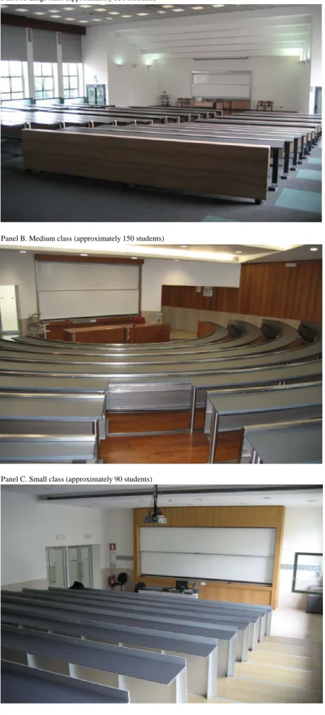
in physical size, classrooms are very homogeneous in terms of both equipment and furniture, i.e. all classrooms have PC’s and overhead projectors and are furnished with essentially the same chairs, benches and desks. Figure A1 in the Appendix shows pictures of a representative small, medium and large classroom to confirm that, despite the difference in size, all other the physical features of the rooms are very comparable.8
Both the 1999/2000 and the 2000/2001 cohorts of Management students (around 1,100) are divided into 8 classes that range in size from 113 to 147, while both the 300 students in Economics and Finance and the roughly 150 students in the Economics major are split in two groups each, with sizes ranging 138 to 158 and from 54 to 94, respectively (Table 2).
Our main measure of class size comes from the student academic records, where the class identifier is reported next to each student’s single exam result. Thus, we can count the number of students in any given cohort and year who have the same class identifier. We call this variable the student count and it corresponds to the number of students who effectively attended the lectures in the same classroom.9
However, we know that this measure of class size differs somewhat from the number of students who were originally given the same class identifier. In fact, from the teaching planning office we obtained the exact number of students who were given the same class identifier at the beginning of each academic year. This is the number of students who were allocated to the same class by the university administration at the beginning of each academic year. We call this variable the number of enrolled students.
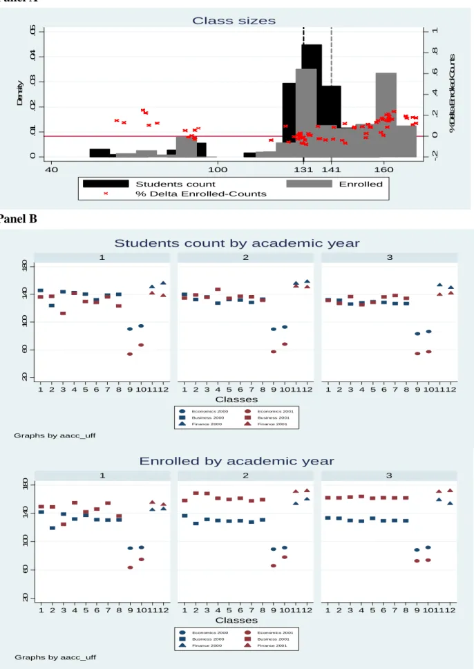
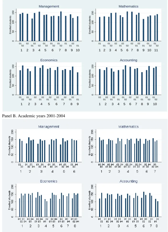
[TABLE 2 and FIGURE 1]
We compare these two measures in Figure 1, Panel A, where the dark and gray bars show the distributions of the student count and enrolled students variables, the dashed lines indicating the respective averages. We also plot the percentage difference between enrolled students and
8
The pictures were taken at the time of writing but similar furniture was available also during the time covered by our data. Namely, the providers of boards, desks and benches, projectors and computers have not changed since then.
9Small variation may come from students taking the exam without attending the lectures or by informally
switching across classes. Both these instances, however, are very limited. Attendance is always strongly en-couraged and (nominally) tightly enforced at Bocconi, especially for compulsory courses. Moreover, attendance levels are monitored both during the academic year, by random visits of administrative attendants, and at the end of the course, with the teaching evaluation questionnaires, that are regularly administered to the students. The data show very high and stable attendance levels. Also, class switching is formally forbidden. Informally switching classes is theoretically possible however, since students are given personalized calendars based on their class allocation, those who want to do so would also have to reorganize their entire schedule.
students counts (the red little x’s) in relation to the number of students originally assigned to that class identifier (on the horizontal axis). Such differences are close to zero (on average about 6%) and they appear to be unrelated to the original official size of class. We also check this relationship by running a simple (unreported) regression of the (percentage) difference between our two measures on the number of officially enrolled students. The estimated coefficient is 0.0006 (with a standard error of 0.0004). In a few cases, however, the differences are larger than 15% (namely in 15 classes out of 72).
Differences between the student count and the number of enrolled students come from students requesting changes to their original class allocation later on in the year, either for the entire year or for some specific courses. Such requests were (and still are) usually very limited and needed to be well motivated. For example, one common reason for such changes are health conditions, that might prevent a student from accessing some parts of the building (e.g. a broken leg) where one’s class is located. However, we cannot rule out a priori that some of these changes are driven by factors like teacher quality or class size, that are endogenous to our process of interest (academic achievement or labor market performance). Additionally, students with different characteristics might be more or less prone to advance such requests, thus complicating the endogeneity issue. For these reasons, in the empirical application we present results produced using both OLS and IV procedure, where we instrument effective class size measured with the student count with the number of officially enrolled students, which, being the outcome of the random allocation algorithm, is purely exogenous. Moreover, the reduced form estimates of our empirical model also have an important interpretation. These estimates are the effect of changing the policy variable that the university administration can more easily manipulate: the number of officially enrolled students. In Section 3 we further discuss our empirical strategy.
In panel B of Figure 1 and in Table 2 we disaggregate the variation in class size, for both student count and enrolled student, at the level of major/academic year/cohort. Overall, there are 12 class identifiers per academic year: 8 classes in Management, 2 in Economics and 2 in Economics and Finance. The average class size (student count) is about 130 (standard deviation 20) students and it does not change substantially over the three academic years. Since students are very unevenly distributed across degree programs, class size does vary across them, with much smaller groups in Economics and larger in Management and Management and Finance.
In all of our analysis, we only exploit the variation in class size within programs and cohorts. As should be clear from the discussion above, the main source of variation in our independent variables is at the level of cells defined by the intersection of academic year, cohort, degree program and class identifier, therefore we will adjust our standard errors accordingly.
Table 3 and Figure 2 summarize the extent of heterogeneity in the classroom and across the 72 different classes.10 There is a non-negligible variation in one’s peer group composition although, as we will show, the amount of heterogeneity we observe is consistent with random assignment of students into classes. For example, the share of females is on average equal to 0.42 with a between class std.dev. of 0.08. Class 11 in the third year of the Finance major, for the 2001 cohort, has a share of 0.23; while class 4 of the first year Business, 2000 cohort has a share of 0.6. The share of high income students is on average of 0.22, with a range of 0.12-0.35. We also detect considerable variation within a major for a given cohort.
[TABLE 3 and FIGURE 2]
In the next section we provide evidence that demonstrates the effectiveness of the random allocation mechanism of students as well as some evidence of the essentially random allocation of teachers to classes.
2.2 Evidence of random allocation
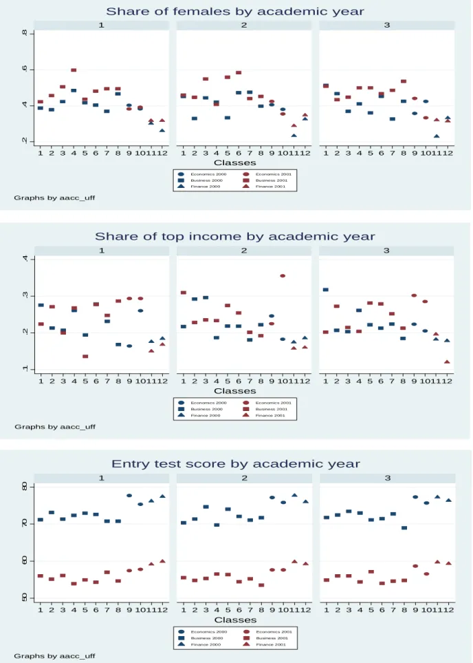
Figure 3 provides evidence consistent with random allocation, as in De Giorgi and Pellizzari (2009) and De Giorgi et al. (2009); and as in Guryan et al. (2009). The figure compares the distributions of entry test scores of the students in the 8 classes of the Management program in each academic year (upper panel). For expositional brevity, all the distributions refer to only one cohort (2000) although the results are similar if we use the other cohort. The middle and lower panels of Figure 3 plot the same distributions for the 2 classes of Economics and Economics and Finance, respectively.
[FIGURE 3]
10
8 Management classes time 3 academic years and 2 cohorts yields 48 cells of variation. Additionally, the Economics and Economics and Finance programs each have 2 classes times 3 academic years and two cohorts for a total of 12 cells each.
As it is evident from the graphs, the distributions look very similar. In Table A3 in the Appendix we report the p-values of a complete battery of Kolmogorov-Smirnov tests for the equality of the distribution of ability in all possible pairs of classes within the same degree program, cohort and academic year. Only in 7 out of the 180 admissible pairs of classes (i.e. 4% of the cases) the distributions are statistically distinguishable at the 95% level.
In order to check for random assignment on other observable characteristics, in Table 4 (Panel A) we report tests for the equality of the mean percentage of female, the mean percent-age of students from top income families and the mean entry test score across classes within each cohort-degree program-academic year cell.11 In none of the cases it is possible to detect differences that are significant at conventional statistical levels.
Finally, in the lower panel (Panel B) of Table 4 we report the coefficients on our two measures of class size (the student count and the number of officially enrolled students) obtained from regressions run at the level of the single class (i.e. with 72 observations in total) and where the dependent variable is either the share of females in the class or the share of students from high income families or the average entry test score. In all regressions we condition on the full (three-way) interactions of cohort, degree program and academic year fixed effects. Results show that in none of the cases class size (regardless of how it is measured) is significantly
correlated with any of the observable characteristics of the student body that we consider and that the reported coefficients are very small in magnitude.
[TABLE 4]
The evidence above and the discussion of the allocation mechanism in Section 2.1 should have convinced the reader that students are indeed randomly assigned to classes and that such allocation was enforced by the administration. Nevertheless, one might still worry that teachers select the size of the class they want to teach. If, for example the best teachers are allocated, either by their own will or by some university policy, to teach smaller classes, our estimates would reflect both the direct effect of class size and the indirect effect of teacher quality. We have several reasons to believe that this concern does not apply to our data. From conversations with the administrators we draw the conclusion that the assignment of teachers was completely
11The reported F-tests are derived from regressions of the mean characteristics of the class on dummies for the
class identifiers, controlling for cohort and academic year fixed effects. The regressions are run using class-level observation, i.e. 48 observation for Management and 12 each for Economics and Economics and Finance.
unrelated to the process of allocating students to classes. In fact, the two processes were carried out by distinct bodies: secretaries in each department would assign teachers to class identifiers and officers in a centralized teaching planning office allocated students to class identifiers.
The available empirical evidence is consistent with this interpretation. Although for privacy reasons we lack data to identify individual teachers, using paper archives from Bocconi we were able to reconstruct teacher identifiers for the teachers of 4 courses in the Management program. Figure 4 shows the size of the classes allocated to these teachers over the academic years 1999-2000 and 1999-2000-2001. On the horizontal axis we report the (anonymized) teacher identifier and the vertical bar indicating the size of each of the classes taught by that teacher in those academic years. For example, teacher 1 in Management taught a class of 142 students in the academic year 1999-2000 and a class of 148 students in the academic year 2000-2001. In Panel B of Figure 4 we show the same data for the following 4 academic years, 2001-2002 to 2004-2005; while the structure of the degree programs changed for cohorts entering after 2000, we believe that the assignment of teachers to classes was similar from in the 2001-2002 to 2004-2005 cohorts. Evidence from these later years is therefore helpful for understanding the assignment of teachers. In those later years, the within teacher standard deviation (accounting classes) in the size of the assigned class is larger than the between teachers variation and indeed quite close to the overall variation. To reiterate a teacher could be assigned 121 students (about the average) in 2001-02 and then 160 students the following year (the second largest class).12 Further, a simple regression, omitted for brevity, of enrollment on teacher fixed effect shows results consistent with the essentially random allocation hypothesis, i.e. no relation between teachers and the size of the class they are assigned to.
[FIGURE 4]
2.3 Survey of graduates
In addition to the administrative records, Bocconi regularly surveys its graduates through a questionnaire administered to every student around one and a half years after graduation (De Giorgi et al. 2009). These surveys focus on the labor market experience of the graduates and contain information on the employment profiles, wages and job satisfaction.
12
In the main analysis we do not pool together data for the academic years 1999-2001 and 2001-2004 because, starting with 2001-2002, the entire structure of the degree programs was changed.
While we view the ability to link detailed information about students while in school with labor market outcomes as an important contribution of our paper, we recognize that there are two potential problems with these surveys. First, the response rates are not particularly high. Overall, we are able to match slightly more than 50% of the students in our cohorts (not unusual for survey data). We believe that these response rates are mostly due to the compulsory military service for men, which males typically completed after graduation. On average only about 34% of them answer the survey as opposed to almost 73% of females. While we are concerned that selection into the survey may bias our results, we can partially alleviate these concerns by comparing results between our two cohorts. Military service was 10 months long and was abolished in 2001 for citizens born after 1985. Although male students in our cohort were born before 1985 and hence were not exempt, in the years prior to the abolition of military service, the set of reasons for which a male could avoid military service expanded. Therefore, the number of people who were required to serve decline substantially between our two cohorts.13 While the response rates for females was similar across the two cohorts, the response rate for males increased from 24% to 47% between the two cohorts.
A second issue relates to the measure of wages, which are recorded in 11 intervals. The large majority of respondents (over 90%) do report wage information, which is asked to anyone who has had at least a job between the day of their graduation and the day of the interview (96% of the respondents). The intervals range from below 750 to over 5,000 euros per month (net of taxes) and are spaced by either 250 or 500 euros. The descriptive statistics (means and standard deviations) reported in Table 1 refer to an imputed measure of wages computed at the mid-point of the interval indicated by the respondent (for the lowest and the highest intervals we take the upper and the lower limit respectively). All monetary values are in euros at current prices. The mean entry wage is around 1,300 euros net per month, corresponding to approximately 1,700-1,800 USD. The mean wage increases over time at a rate (around 9%) higher than inflation. While Economics and Management students seem to be earning comparable salaries, Economics and Finance shows a wage premium of about 15%, although these differences easily disappear once controlling for individual characteristics.
13For example, around the year 2000 a set of new rules allowed permanent exemption from the service to
3
Empirical Strategy
The existing literature on class-size and class heterogeneity has mostly exploited natural exper-iments as source of identification. There are, however, a few notable exceptions, i.e. Krueger (1999), Krueger and Whitmore (2001), Duflo et al. (2008 and 2009).
In this work, we exploit the experimental variation arising from the random allocation of students to classes followed at Bocconi University. As we discussed in Section 2.2, students are randomly assigned to the same class identifier for all the courses of a given academic year, i.e. they sit the entire year with the same peers. The allocation is, then, repeated at the beginning of each academic year. Given that, for the most part, students allocated to the same class attend lectures in the same physical classroom, the definitions of class, classmates and classroom coincide in our framework.
This random allocation produces exogenous variation in the size and composition of classes and therefore allows us to cleanly identify the effect of class size and heterogeneity on academic performance and labor market outcomes. Variation in the size of the class is generated mostly by differences in the physical capacities of the classrooms in the different university buildings and can, thus, be considered exogenous to other inputs in the education production function. In particular, all classrooms have exactly the same equipment and the same furniture, while larger classrooms have obviously larger blackboards and screens.
In the next section, we explore the effect of class size and class heterogeneity on both aca-demic performance and labor market outcomes. Here we briefly discuss our empirical strategies for the identification of these two effects.
Let us start with academic performance. To avoid complications due to the endogenous choice of elective courses, we concentrate exclusively on compulsory courses that, for all of the three programs that we consider, take up most of the students’ time over the first three academic years. Over this period, students are randomly allocated to different classes three times, one at the beginning of each academic year. Hence, in our empirical specification we use the average grade in the courses of each academic year as a measure of student performance and we regress it on the size of the class in each year. Eventually, we have three observations for each student, thus, we can control for individual effects as well as for year and program effects. Notice also that, since the average grade per academic year is computed over a slightly
different number of courses across degree programs and academic years, we weight observations accordingly.14
We derive our empirical specification from the following model:
yijtcd=α sizejtcd+ηi+γtcd+uijtcd (1)
whereyijtcd is the average grade of student iin classj, yeart, cohort cand degree programd,
sizejtcd is the size of the class j in the same tcd cell, ηi is an individual fixed effect, γtcd is a
fixed effect that varies by year-cohort-program cells anduijtcd is a residual random term.
The possible endogeneity in our empirical measures of class size may impede identification of equation 1 if students defy the random assignment and change classes in a way that is correlated with teacher quality or class size. To describe the nature of the potential endogeneity ofsizejtct,
assume that the random term uijtcd is the sum of an unobservable class component ζjtcd that
is common to all students who are allocated to class j in the tcd cell and a purely random idiosyncratic termvitcd:
uijtcd=ζjtcd+vijtcd (2)
The most obvious interpretation of ζjtcd is teacher quality, but it could represent any class
specific unobservable shock.
Then, the student countsizejtcd results from the aggregation of the individual re-allocation
decisions of all the students in the same cohort and degree program. Students who were originally allocated to class j may decide to switch class, while others who were originally allocated elsewhere may request to be moved to class j:
sizejtcd =enrolljtcd+ X i3j inij− X i∈j outij (3)
whereenrolljtcd is the number of students originally allocated by the administration to class j
in the tcd cell, inij is an indicator function that is equal to 1 if student i (who was originally
allocated to a class different from j) moves to class j and outij is an indicator function that
takes value 1 if student i(originally allocated to classj) manages to be moved elsewhere.
14Each student-year observation is weighted by the number of exams taken by the student in that specific
academic year. Table A1 in the Appendix shows that there is some small variation in such number across degree programs and years.
The key endogeneity concerns arise because the functionsinij andoutij might be influenced
by ζjtcd, i.e. teacher quality in class j (or any other class-specific shock). More formally, we
can define the two functions as follows:
inij = f(Xijtcd, ζijtcd) (4)
outij = g(Xijtcd, ζijtcd) (5)
whereXijtcd is a set of observable characteristics of theij pair in the tcdcell andζijtcd can be
interpreted either as a single unobservable shock or as a vector of unobservable characteristics of the ij in the sametcdcell.
In this setting, applying simple OLS to equation 1 does not produce consistent estimates of the parameters, particularly ofα. The OLS orthogonality assumption fails becauseE(sizejtcd, uijtcd)6=
0. In fact, as equations 3, 4 and 5 demonstrate, the unobservable class shock ζjtcd is both a
determinant of sizejtcd and a component of the error termuijtcd of equation 1.
However, this discussion also clarifies that enrolljtcd is a perfect instrument for sizejtcd in
equation 1, so that consistent estimates of its parameters can be produced with an instrumental variable approach. In fact, while the observed class size may be correlated with the error term,
E(sizejtcd, uijtcd) 6= 0, enrolljtcd is merely the outcome of the random allocation algorithm,
hence it is exogenous by construction andE(enrolljtcd, uijtcd) = 0. At the same time, equation
3 clarifies thatenrolljtcd andsizejtcd are correlated. Theoretically, if the process of reallocation
of students across class was pervasive,enrolljtcd could potentially be a weak instrument. Given
what we know from discussions with the university administrators and from our analysis of the raw data in Section 2.1, we do not expect this to be a serious concern. In fact, the results of the first stage regressions of all the specifications that we present in Section 4 confirm this expectation (the F-tests of the excluded instruments range from 51 to 7,000). Our solution to this identification problem resembles closely the approach of Krueger (1999).
Although we useenrolled students primarily as an instrument forstudent count, the reduced form estimates are interesting in their own right, as they may be interpreted as the relevant policy effect from the perspective of a university administrator. In fact, while changing the number of officially enrolled students (enrolled students) is a relatively easy task, the enforce-ment and manipulation of the actual (size) student count would depend on the university’s
enforcement capabilities, which might vary across colleges. At a minimum, the reduced form estimates are of interest to Bocconi’s administrators.
Regardless of how we measure class size (student count or enrolled students) or the esti-mation procedure used (OLS, IV or reduced form), the computation of the standard errors of the estimated coefficients from equation 1 for correct inference poses some additional problems. First, the individual fixed effectηi induces correlation across the observations that refer to the
same student. Second, we also need to cluster the standard errors to take into account the fact that students in the same class-year-cohort-program cell share the same class sizesizeijtcd. We
address the first problem by transforming the model in orthogonal deviations, a transformation that allows to eliminate the individual effect ηi from the equation and, in a standard setting,
it also preserves homoskedasticity.15 In the specific case of equation 1, homoskedasticity is not guaranteed in the transformed model because class size does not vary at the same level of the dependent variable. In fact, while academic performance varies at the level of the single student and across academic years, class size is constant for all students who are allocated the same identifier within the same year-cohort-program group. Hence, we cluster the standard errors of the transformed model at the correct level of the class-year-cohort-program cell (there are 72 such cells in total).
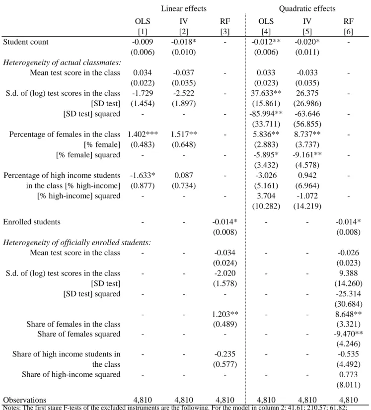
In Section 4.1, we investigate the effect of class size on academic performance using a series of variants of equation 1: we look at heterogeneity of the effect of class size across different types of students and we also consider the effect of class composition on academic performance, in this latter case measures of class heterogeneity are added to 1. In all cases, the empirical strategy for the estimation of equation 1 and its variants remains the same. When we investigate the effect of class heterogeneity, we construct the instruments for the actual class composition using information from the university administration about the original official class allocation of each single student and we construct the corresponding measures of heterogeneity (e.g. share of females) among students who were officially allocated to the same class.
In Section 5 we also look at the direct effect of class size and class composition on labor market performance. In this case the choice of the empirical model is less obvious. While we observe only one outcome for each student (their wage after entering the labor market),
15
Orthogonal deviations are computed as the difference between the individual observation and the mean of all future observations for the same individual, see Arellano (2003).
we observe at least three different class sizes for each student over the course of her academic career (usually more than that if one takes elective courses into account). We choose the most obvious specification, where we include the average class size (size) a student has been exposed to according to the following equation:
wicd =β sizeicd+δXicd+icd (6)
wherewicd is the wage reported by studentiin cohortcand degree programd,mean(size)icdis
the average of the 3 class sizes a student has experienced in her first three academic years and Xicdis a large set of controls determined prior to a student’s matriculation that include gender,
the score obtained in the cognitive entry test, household income, geographical residence, type of high school, plus controls for survey wave, cohort and degree program fixed effects.
Similarly to equation 1, identification rests on the random allocation mechanism and we address the potential endogeneity with the same approach discussed above. The standard errors are clustered at the same level of variation of mean(size)icd, i.e. the intersection of
cohort, degree program and the three class identifiers of each academic year.16
4
The effect of class size and class composition on academic
performance
4.1 Academic Performance
In this section we analyze the effect of class-size on academic performance. We estimate equation 1 both by OLS and IV, to account for the possible endogeneity in the class size measure as given by the student count. Later (Section 4.1.1) we also investigate the interaction of class size with the individual characteristics of the student, to test whether some type of individuals benefit or suffer more from smaller classes. Finally, in Section 4.1.2 we estimate the direct effect of class composition on academic performance.
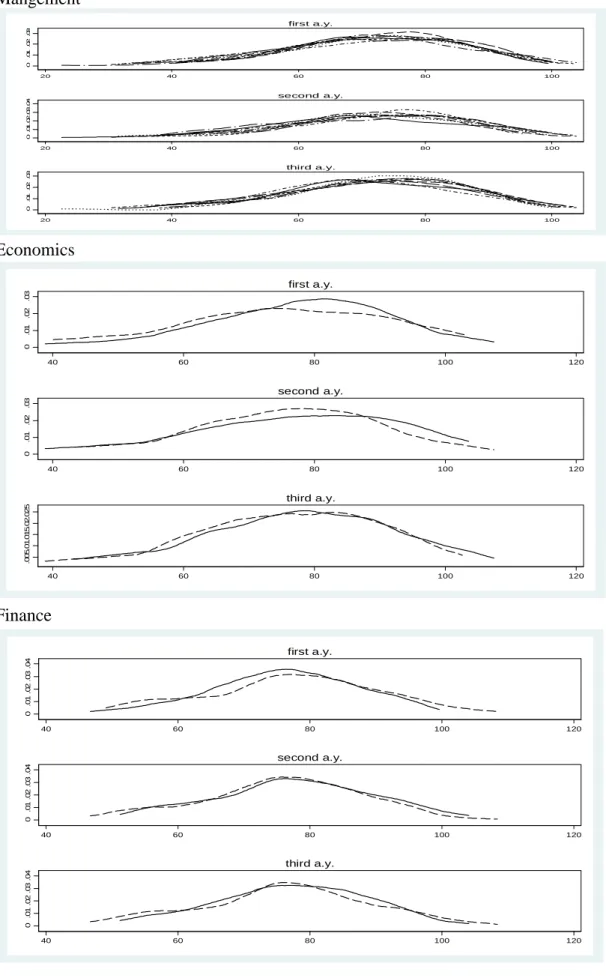
Table 5 reports our main results. Using a simple linear specification (columns 1 to 3) we find a significant effect of class size on academic performance. The OLS estimate in column 1 indicates that one additional student in the class reduces the individual mean grade in the
16
corresponding academic year by 0.01 grade points over an average of 26 (which corresponds roughly to a B+ for US universities). The IV estimate is a bit larger in magnitude and equal to -0.017, although it is not statistically different from the OLS. As we expected, the F-test of the first stage is very strong (F-stat of 241) and it allows to rule out the usual concerns due to weak instruments. Finally, the reduced form estimate is in between the OLS and IV.
To put the magnitude of the estimated effects into a better perspective, take the IV co-efficient and consider the effect of increasing class size by one standard deviation (computed over the entire sample), which corresponds to approximately 20 students or about 15% over an average class size of around 131. Such a change would reduce the mean grade by about 0.34 points or about 0.15 of a standard deviation, an effect that is consistent with the existing literature that finds significant effects (see Angrist and Lavy (1999), Krueger (1999), Bandiera et al. (2008), Pinto Machado and Vera-Hernandez (2009)).
[TABLE 5]
In the following columns 4 to 6 of Table 5 we explore the presence of non-linearities in the effect of class size on student performance. In a setting where class size is one of the inputs of a standard human capital production function with decreasing return to scale, we should find that the impact of class size flattens out at larger sizes. In columns 4 to 6 of Table 5 we modify our specification and estimate a spline regression where we allow the effect of class size to vary at each quartile of the distribution. We estimate such model both by OLS and IV and in column 6 we report the reduced form. In none of these three specifications it is possible to detect significant differences in the slope of the relationship between class size and academic performance across quartiles of the distribution of the regressor.17
The lack of non-linearities highlighted in Table 5 suggests that a possible coherent mech-anism for explaining the class-size negative effects even in large classes is that suggested by Lazear (2001), where students are subject to disruption shocks that hit one single student and then propagate by disturbing the entire class (or students in a neighborhood of who is first hit). In that setting, the class size effect is indeed negative in the size of the class even for large classes if the probability of no-disruption is large, as one would expect among college
17Notice that the coefficients in columns 4 to 6 of Table 5 measure the difference between the slope of the
regression at each quartile compared to the previous one. The coefficient on the first quartile is the actual slope. The search for non-linearities has been also performed using a quadratic polynomial, those results are in line with the ones presented in the paper.
students.18 One can think of the an education production function with the existence of public goods, indeed disruptions and meaningless questions do have the features of public goods and negative externalities.
Although the evidence in Table 5 suggests that the effect of class size on academic perfor-mance is essentially linear, it must be noted that it is very hard to speculate on the functional form of the production process without knowledge of the true objective function of the univer-sity and the possible constraints it may face (Hoxby, 2000).
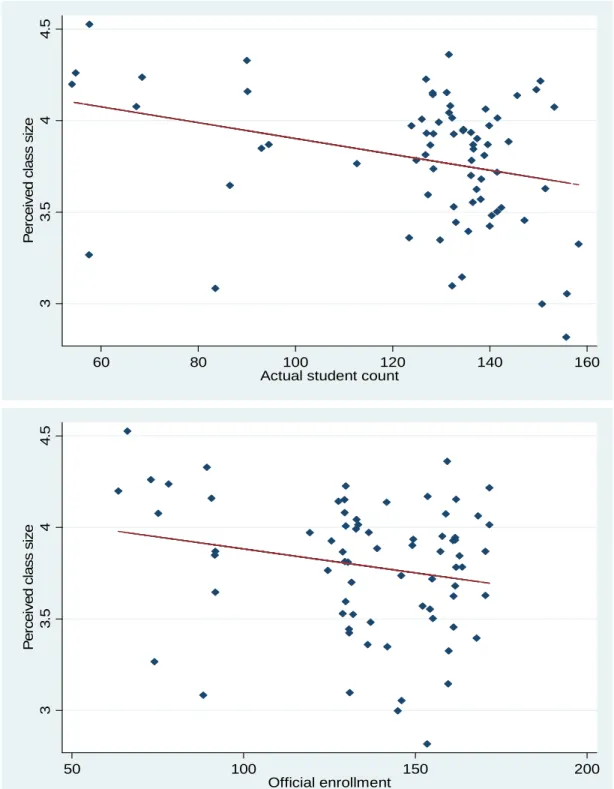
To conclude this section we present some simple evidence to show that students themselves do have the perception that larger classes are detrimental to their learning. As it is now custom-ary in most universities, Bocconi regularly administers evaluation questionnaires to its students to gather their opinions about various aspects of the teaching environment. In particular, the questionnaire that was administered to the students in our sample includes a question on the size of the class. Specifically, students are asked to indicate on a scale from 1 (disagree) to 5 (agree) if they agree with the following statement: ”the number of students in the classroom allows all the teaching activities to be regularly and efficiently carried out.” In Figure 5 we plot the average answer to this question in each of the 72 class-year-program-cohort cell against the corresponding class size measured either by the students count (upper panel) or by the number of officially enrolled students (lower panel). As the figures clearly show there two variables are negatively (and significantly) correlated, although the R-squared of these simple regressions are relatively small (9.3% when the students count is used as a measure of class size and 4.3% when we use the number of officially enrolled students).
[FIGURE 5]
4.1.1 Heterogeneous effects
After having established that class size reduces student achievement, we now explore the het-erogeneity of the effect across students of different ability (as measured by the pre-enrollment admission test), gender, and family income. These results are interesting for at least two reasons. First, studying the heterogeneity of the effect is informative of the distributional con-sequences of lowering class size. If, for example, students from poorer families benefited more
18
Borrowing from Lazear (2001), if the probability that a student is not disrupting her or others learning isp
then the probability that disruption takes place in a classroom ofnstudents is 1−pn, which behaves essentially linearly whenp→1 even when the class-size is between 1 and 200 students.
than others, reducing class size could be an efficient means of redistribution. Second, if school administrators face a budget constraint and cannot provide small classes for all students, they may want to allocate spots in small classes to students who are likely to benefit the most.
Table 6 reports the results that we obtain by augmenting our basic specification (columns 1 to 3 of Table 5) with interactions of class size and three crucial characteristics of the students: ability, gender and income. The OLS estimates are never significant, while in both the IV and the reduced form estimation we find that the negative effect of larger classes essentially disappears for female and students from wealthier families.
[TABLE 6]
One possible explanation, for the above results is that students from wealthier families are less affected by large classes because they have additional resources from their families that can be used to compensate for less effective lectures (better textbooks, better study environment, remedial private teachers, et.). Given that females have a more pro-social behavior in general (they drink less (Sloan et al., 1995), they smoke less (Gruber, 2001), they commit less crime (Ludwig, 2001)), they may also be less disruptive in the class and, if there is some degree of clustering of study mates across gender, they may suffer less from disruption because they sit close and interact more with other girls than other boys, who disrupt more.19 This interpreta-tion, although still speculative, would also be consistent with the results that we obtain in the next section on class composition. A puzzling result is that the OLS estimates appear to be all insignificant while the IV results on class-size are similar to the earlier ones although with larger standard errors.
4.1.2 Class Heterogeneity
In this section we explore how the heterogeneity of a student’s peers influences her academic performance. This exercise is interesting for at least two reasons. First, growing evidence suggests that the composition of one’s peer group is an important determinant of individual behavior and in particular of students’ achievement.20 Further, recent evidence in Duflo et al. (2008) shows that tracking has positive effects on students’ performance; in the same spirit
19The literature also documents that women are more risk averse (Schubert et al., 1999) and “shy-away” from
competition (Gneezy et al. (2003).
Pinto-Machado and Vera-Hernandez (2009) find positive and heterogeneous effects of peers ability on student performance. Cooley (2009) finds evidence of peer effects on performance within race-based reference groups. Here, we investigate whether the composition of classmates in terms ability, income and gender affects student performance. We compute a measure of dispersion for ability, income and gender for each class. Because of the process of repeated random allocation that we described earlier on (Section 2.1), each student is exposed to a different set of randomly selected peers in each academic year. For each of these groups, we compute the fraction of female in the class, the fraction of students from high income families and the mean and the standard deviation of the log entry test score for those effectively in the classroom (similarly to the student count definition).21 Further, having obtained from the administration the original class identifier assigned to each student by the random allocation mechanism, we can produce the same measures of class heterogeneity based on this purely exogenous and theoretical class composition (similarly to what we do for the enrolled students measure). Hence, in Table 7 we report both the OLS, IV, and reduced form estimates.
[TABLE 7]
In columns 1 to 3 we concentrate on a simple linear specification and we find that a larger share of female students in the class is beneficial for academic achievement: increasing the percentage of females in an average class (which is approximately 40% female) by 10 percentage points increases gpa of the average student by 0.14-0.15 of a grade points or 0.05-0.06 of a standard deviation. Increasing the fraction of high-income students has the opposite effect: adding 10 students of this type to an average class (which has approximately 28 out of 130 students) reduces the gpa of the average classmate by 0.16 grade points or 0.07 of a standard deviation, although this effect disappears in both the IV and the reduced form specifications.
In the following columns 4 to 6 of Table 7 we experiment with a simple quadratic specifica-tion to determine if the effects of class composispecifica-tion appear linear. In the OLS results, both the linear and the quadratic effect of the dispersion in ability (measured by the standard deviation of the log entry test score) are significant, suggesting that more diverse classes perform better but such effect is decreasing. The results for gender composition are qualitatively similar: a
21Notice that the mean proportion of females and high income students are sufficient statistics for the
distri-bution of these dichotomous variables within each class. The entry test score, instead, is a continuous variable therefore we compute both the mean and the standard deviation.
higher fraction of female in the class increases performance at a decreasing rate. Finally, the incidence of high income students still has no impact on performance. In columns 5 and 6, we replicate the estimates using our IV and reduced form specifications. Here, only the effects of gender composition remain significantly different form zero, although the sign and magnitude of the test score results is broadly similar across specifications.
Our results for gender composition show the importance of estimating non-linear effects. The results from the linear specification, columns (1) - (3), suggest that for our sample, increas-ing the share of female students increased performance. Because the students in our sample are predominately (58%) male, these results are consistent with at least two different hypotheses: (a) students always learn better when the share of female students increases (b) students tend to learn best when the ratio of males and females is approximately even. Our quadratic results cast doubt on (a). Taken at face value, these coefficients suggest that the-student optimal gender composition is 49.4% female.22
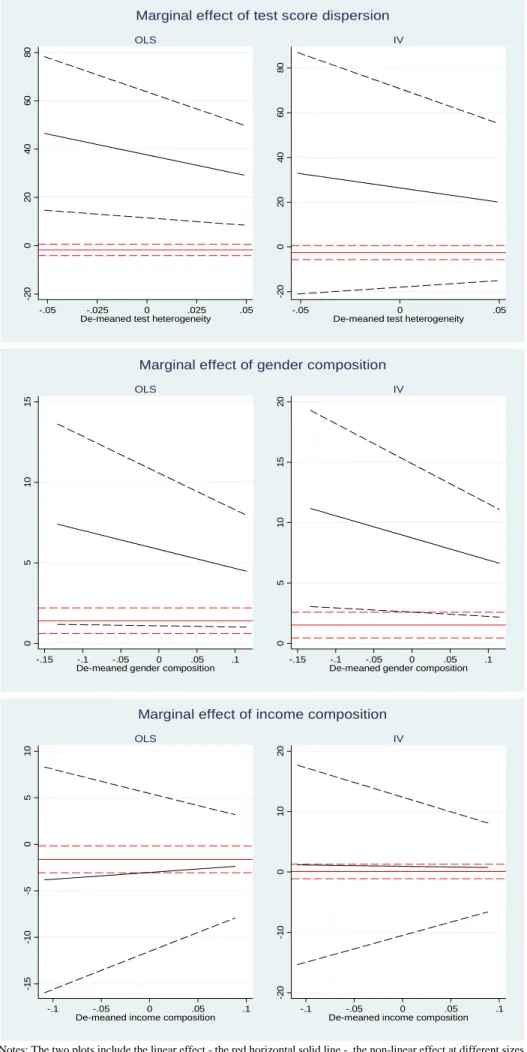
To give a sense of the magnitude of these non-linear estimates, Figure 6 plots the marginal effects of our three measures of class composition (dispersion in ability, gender composition and income composition) derived from both the linear (corresponding to the estimates in columns 1 to 3 of Table 7) and the quadratic (corresponding to the estimates in columns 4 to 6 of Table 7) specifications. In the left panels of Figure 6 we show the OLS results while the IVs are plotted in the right panels.
[FIGURE 6]
The OLS quadratic effect of the dispersion in test scores (top left panel) shows that increas-ing the diversity in ability among classmates by one standard deviation (approximately 0.015) from the mean increases performance by 0.56 of a grade point or 1/4 of a standard deviation. Performing the same exercise, i.e. increasing test dispersion by one standard deviation, starting from an already diversified class, say one with dispersion in ability that is 2 standard deviations above the mean (corresponding approximately to the top 5% of the distribution), increases per-formance by 0.48 of a grade point, that is about 15% less than before. The entire effect of test score dispersion, however, disappears under the IV specification due to large standard errors.
22The baseline results suggest that the effect of share female are given by: 5.836·(share female)−5.895·
Our results clearly show that gender composition has a robust and large effect on perfor-mance. The estimate on share female remains significant in all specifications: OLS and IV, linear and quadratic. The marginal effects are plotted in the middle panels of Figure 6. Let us focus on the IV specification (although the OLS estimates are not substantially different) and notice that increasing the percentage of female classmates by one standard deviation (ap-proximately 0.04) from the mean (which is equal to about 40%) increases performance by 0.23 of a grade point or 10% of a standard deviation. Performing the same exercise, i.e. increasing the incidence of females by one standard deviation, starting from a class that is already female dominated, say one with female incidence that is 2 standard deviations above the mean (cor-responding approximately to the top 5% of the distribution), increases performance by 0.19 of a grade point, that is about 17% less than before.
The results for income dispersion are significant only in the linear OLS specification and indicate that a larger share of high income classmates reduces performance. However, such effect disappears in all other specifications.
Once again, the interpretation of these results is merely tentative and speculative. However, the positive effect of the incidence of female students in the class seems consistent with the idea that girls have a more pro-social behavior and, thus, may also be less disruptive. Along the same line, one may try and rationalize the negative effect of wealthier students by arguing that, given their ability to make up for less productive lectures with private resources, they may be more prone to disruption to the detriment of the entire class. The positive effect of dispersion in ability seems to indicate that students’ skills are complements in the classroom production function.
The non-linearities in some of these effects open up the possibility to reshuffle students in classrooms and increase average performance without necessarily requiring additional resources. We return to the issue of optimal class formation in Section 6.
5
The effect of class size on labor market performance
In this section we test whether the negative effect of class size in terms of academic performance affects the labor market outcomes, around one a half years after graduation. The literature on school resources and labor market performance (Moffit, 1996; Hanushek, 2006) finds a
substantial positive effect of school resources, measured as class-size or teacher per pupil ratios. As explained in Section 2.3, we observe our students once they graduated, typically around one and a half years after graduation and, although we have no longer term outcomes, we believe that it is quite important to study the short-run impacts, as discussed by Oyer (2006).
Given that our students are assigned to a different class in each of the 3 years of required courses, the most natural way to specify our empirical model is to consider the average of those 3 class sizes as our measure of treatment. The results reported in Table 8, where we produce estimates of equation 6 using a variety of specifications. In columns 1 and 2 we adapt the estimation procedure to the original wage information (recorded in intervals), and we apply interval regression. To avoid the technicalities involved in adopting an IV procedure in this model, we only report results computed using either the students count or the enrolled students as a measure of class size. In the following columns (3 to 5) we use as a dependent variable a continuous version of the wage information computed at the mid points of the intervals indicated by each respondent. Then, we can apply the standard techniques and we report OLS, IV and reduced form estimates.
The estimates reported in the first 5 columns of Table 8 indicate that the effect of the average class size in college on entry wages is negative and of non-trivial magnitude across all specifications.
[TABLE 8]
The magnitude of the coefficients suggests that an increase of 20 students in the size of the average class would reduce monthly wages by 90 to 95 euros on average or around 115USD or 7% over the average monthly wage. This is quite a significant effect, particularly if such a penalty is never recovered over the course of one’s working life, as suggested by Oyer (2006). In the last 5 columns of Table 7 we repeat all the estimates by conditioning on academic performance. Interestingly, the magnitude of the effects decreases by a mere 7%, suggesting that class size affects labor market outcomes both through its impact on academic performance and also independently through some other mechanism, possibly the development of non academic skills.23
6
The
optimal
class allocation
A crucial policy question is whether an optimal class can be designed by the administrators in terms of size and composition. We address this question given the estimated parameters from Section 4.1. First, we must take a stand on the planner’s objective function and on the constraints she faces. For simplicity, we assume that the planner seeks to maximize the sum of individual performances. We recognize that there are many other reasonable objective functions. The planner may be concerned with equity or an objective, such as encouraging interaction between men and women, that is not captured in academic performance. We further assume that the total number of classrooms and teachers, the size of each classroom, and the student population are fixed. This assumption corresponds to solving the short run problem where resources are fixed. If we solved the problem multiple times with different resources and populations, these results would also help the social planner optimally allocate resources to higher education. Here, the planner will therefore change the type of students in each classroom, keeping the number of classes fixed.
Let’s write studenti performance in classj as follows:
Pij =αsizej +β1f emalej+β2f emale2j +γ1σ(ability)j+γ2
σ(ability)j
2 .
So that the planner’s objective function is:
X j wjPj =α X j wjsizej+β1 X j wjf emj+β2 X j wjf em2j+γ1 X j wjσ(abil)j+γ2 X j wj(σ(abil)j)2 =M
wherewj is the size of class j. Hence the full program is:
max f em,σ(abil) M =α X j wjsizej+β1 X j wjf emalej +β2 X j wjf em2j +γ1 X j wjσ(abil)j+γ2 X j wj(σ(abil)j)2 s.t. N =N sizej =Nj E[f emj] = F N =f abili ∼Φ(abil).
Where Φ is the appropriate cdf. A simple example will help clarify how our estimates can inform the allocation of students into classes based on gender. Assume that administrators have three classrooms that are fixed in size. Let these sizes be given by N1, N2, and N−N1−N2 respectively. To simplify the analysis so that it focuses specifically on the gender margin, assume further that ability does not influence performance (γ1=γ2 = 0) , or that the ability of males and females is drawn from an identical distribution and that the planner does not know an individual’s ability. Since we have fixed the size of classroomj to beNj, we can re-write the
problem as solving for the share of females in each classroom (fj = NFj
j) rather than the number. This transformation ensure that our results are directly comparable to our empirical section. We need to define only J −1 classrooms as the J −th one would be just the complement to N. Let’s also definef = FN as the fraction of females in the population of interest.
The solutions to this problem are:
f1∗ = 2β2n1F −β1N(1−n1(3−2n1−2n2)−2n2(1−n2)) 2β2N(1 + 2n1(n1+n2−1) + 2n2(n2−1)) , f2∗ = 2β2n2F −β1N(1−n1(2−2n1−3n2)−2n2(1−n2)) 2β2N(1 + 2n1(n1+n2−1) + 2n2(n2−1)) , f3∗ = f−f ∗ 1 −f2∗ 1−n1−n2 .
For example, where N = 1000, F = 400, n1 = .5, n2 = 1/3, n3 = 1/6, with the estimated βb1 = 5.836,βb2 =−5.895 would give f1∗ =.37, f2∗ =.41, f3∗ =.46 andF1∗ = 186, F2∗= 138, F2∗= 76.
The same type of optimization can be performed taking into account the heterogeneity in ability, as well as changing the number classrooms, obviously one would need to take into account the actual joint distributions of the choice variables. Further, although we fixed the student body in this exercise nothing prevent an institution from adjusting along several dimen-sions subject to some possible budget constraints. For example, from our analysis it is obvious that a larger share of female students would benefit the overall performance, indeed given the parameters we estimate we know that the share of females which maximize performance is given by the ratio−cβ1
2cβ2
![Table 5. Class-size effects on academic performance OLS IV RF OLS IV RF [1] [2] [3] [4] [5] [6] Student count -0.010* -0.017* - - - -(0.005) (0.009) Enrolled students - - -0.014* - - -(0.007)](https://thumb-us.123doks.com/thumbv2/123dok_us/10823454.2970780/40.1188.140.1021.122.696/table-class-effects-academic-performance-student-enrolled-students.webp)