The spatial distribution of economic activities in the European Union 1

1

The spatial distribution of economic activities in the

European Union

Pierre-Philippe Combes

& Henry G. Overman

11

July 2003

Abstract: This paper considers the spatial distribution of economic activities in the European Union.

It has three main aims. (i) To describe the data that is available in the EU and give some idea of the rich spatial data sets that are fast becoming available at the national level. (ii) To present descriptive evidence on the location of aggregate activity and particular industries and to consider how these location patterns are changing over time. (iii) To consider the nature of the agglomeration and dispersion forces that determine these patterns and to contrast them to forces acting elsewhere, in particular the US. Our survey suggests that much has been achieved in the wave of empirical work that has occurred in the past decade, but that much work remains to be done.

JEL Classification: F14, F15, R12

Key words: Location, European Union, descriptive statistics, empirical studies

1

This paper is a draft chapter for the forthcoming Handbook of Urban and Regional Economics, Volume 4, Vernon Henderson and Jacques Thisse (eds.) We thank Gilles Duranton, Vernon Henderson, Thierry Mayer, Giovanni Peri, Diego Puga, Bertrand Schmitt, and Jacques-François Thisse for very useful discussions. We also thank seminar participants at NHH, a CEPR conference in Paris, and a CEPR Economic Geography Network meeting in Villars. This paper was produced as part of a CEPR research network on ‘The Economic Geography of Europe: Measurement, Testing and Policy Simulations’ funded by the European Commission under the Research Training Network Programme (Contract no: HPRN-CT-2000-00069).

2

CERAS and Boston University. CNRS researcher also affiliated with the Centre for Economic Policy Research. Boston University, Economics Department - 270, Bay State Road - Boston, 02215 MA, USA. [email protected]. http://www.enpc.fr/ ceras/combes.

3

Department of Geography and Environment, London School of Economics, Houghton Street, London WC2A 2AE, United Kingdom, [email protected], http://cep.lse.ac.uk/~overman. Also affiliated with the Centre for Economic Policy Research, and the Centre for Economic Performance at the London School of Economics.

2

1. Introduction...3

2. Data for studying the spatial distribution of economic activity in the European Union...4

3. Facts about the spatial distribution of economic activity in the European Union...8

3.1. Aggregate economic activity and the EU core-periphery pattern ...8

3.1.1. Regional incomes ...8

3.1.2. Accessibility ...10

3.2. Concentration and specialization in the EU...12

3.2.1. Standard methodology ...12

3.2.2. Specialisation patterns across EU countries...18

3.2.3. A mixed picture for regional specialisation ...20

3.2.4. A mixed pattern for industrial concentration ...22

3.2.5. The characteristics of spatially concentrated industries...24

3.3. Comparing the EU and the US: A role for micro-geographical data? ...28

3.4. Where we stand ...33

4. Explanations ...33

4.1. A brief survey of location theory and its application to the EU...34

4.1.1. Theories of space and location ...34

4.1.2. Agglomeration and dispersion forces ...35

4.1.3. The determinants of agglomeration and dispersion forces ...36

4.2. Industrial localisation in the EU ...37

4.2.1. Trade based approaches ...37

4.2.2. Dixit-Stiglitz based approaches ...40

4.2.3. Cournot competition based approaches...41

4.2.4. Where do we go from here? ...43

4.3. Labour productivity and wages inequalities ...44

4.3.1. Labour productivity...45

4.3.2. Wages ...47

4.3.3. Monopolistic competition based approaches ...49

4.3.4. Where do we go from here? ...53

4.4. The dynamics of localisation in the EU...54

4.4.1. Long-run growth ...54

4.4.2. Short-run dynamics and endogeneity controls ...57

4.4.3. What we learn and a comparison with the US ...58

5. Conclusions ...59

3

1. Introduction

This chapter considers the location of economic activity across the European Union (EU). It complements the two chapters on North America (Holmes and Stevens) and ASEAN (Fujita, Mori, Kanemoto, and Henderson) in this volume.

From the chapter by Holmes and Stevens it is clear that, for North Americans, the titles of these three chapters hark back to an earlier period when economic geographers produced maps and studied the detailed location patterns of particular activities, and the detailed activity patterns of particular locations. For Europeans too, such titles evoke a rich history of area based studies from authors as diverse as Christaller (1933), Engels (1845) and Marshall (1890). However, in strong contrast to the North American experience, these titles also speak to a more recent period in which a distinct literature on spatial location in the EU pursuing broader objectives has re-emerged. This chapter surveys this literature.

Before proceeding, it is interesting to consider why European researchers seem to have taken such a different path from their North American colleagues. Our review of the literature points to three key factors. First, the ongoing process of EU integration and its likely impacts have made understanding the evolution of EU production patterns an important policy issue. Second, researchers in the EU have embraced models incorporating increasing returns to scale as the theoretical basis for understanding this evolution. With the development of the New Economic Geography, this has lead researchers to refocus on the spatial impact of continuing integration, and hence spatial location patterns more generally. But this combination of political impetus and theoretical development is not sufficient to explain why European economists have returned to area based approaches. Taken on its own, this only points to a renewed interest in location issues, but does not suggest a uniquely European perspective is necessary. The third factor which has pushed researchers towards a European area based approach is the feeling that the EU is somehow different from the US and that this urges caution in applying existing evidence (usually North American) to understanding European issues.

This brief discussion raises the question of how this EU area based approach should inform the development of regional and urban economics more generally. In an ideal world, the answer to this question would determine what papers appear in this chapter of the book and what papers should be dealt with elsewhere. The main bulk of this chapter would deal with describing the location of economic activity in the EU. Our explanation of these patterns could then draw widely on other chapters in the handbook, leaving us to consider in depth only material that helps us understand why things in the EU might be different. In reality, of course, things do not turn out to be that simple.

The first problem is that many papers that are basically area studies portray themselves as tests of theories of New Economic Geography or location theory more generally. The authors of these papers tend to be annoyed when the main body of regional and urban economics ignores their contributions in favour

4 of papers based on other areas (usually North America). Often this is portrayed as a form of cultural imperialism by our American colleagues. We consider these papers in some depth here with a view to doing two things. First, identifying exactly what they do tell us about the spatial distribution of economic activity in the EU. Second, arguing that they cannot tell us much about location theory more generally because data problems and methodological errors mean they are less informative about theory than papers published elsewhere. The second problem relates to a somewhat smaller body of literature and is in some ways the mirror image of the first. A number of papers use EU data in ways that do tell us things about location theory more generally, but then tend to be ignored because they get labelled as area based and are thus considered too specific for a broader audience. We also consider these papers here and try to spell out what a broader audience may learn from them. The reader should note that this focus tends to move us away from the more descriptive work in the two companion chapters and thus involves considerably more discussion of econometric issues than is found there.

Before outlining the structure of the paper, a comment on what we do not cover. We will not consider national or regional convergence in the EU, innovation, or FDI and trade as these literatures are considered elsewhere in this handbook, by Magrini and Quah, Audretsch and Feldman, and Head and Mayer, respectively. In addition, we only cover the EU as it now stands, with no consideration of the economic geographies of the 10 countries that will join the EU in the next two years.

Turning to what we do cover, the rest of the chapter is split in to three parts. In the first, we consider the main sources of data for studying EU location patterns. This survey is brief and less helpful than it could be reflecting the woeful state of pan-European national and sub-national data. The second part describes the location of economic activity in the EU. This focuses on three key aspects. First, the pattern of overall agglomeration as reflected in differences in regional GDP and GDP per capita. Next we consider the specialization patterns of particular areas and the concentration patterns of particular activities at both the national and sub-national level. We also consider the characteristics of spatially concentrated industries. Finally, we show how micro-geographic data may be used to compare spatial patterns in the US and the EU. The third part of our survey considers the literature that seeks to explain location patterns in the EU. After a very brief theoretical survey, we focus, in turn, on spatial inequalities in terms of industrial localization, labour productivity, wages, and growth.

1. Data for studying the spatial distribution of economic activity in

the European Union

In this section, we consider the data that are available for studying the spatial distribution of economic activity in the EU. After reviewing the literature, and given our first hand knowledge, the only conclusion that we are able to reach is that the European data are a mess. It is not clear where blame for this situation lies. It is clear that part of the problem stems from the institutional framework within which most EU

5 governmental statistical agencies work. In particular, the fact that they often have no mandate to facilitate the re-use of data collected to fulfil their institution roles. Even where they do have a mandate, data are often expensive and incentives to ensure efficient delivery appear to be limited. It is clear that these barriers could be removed, but this would require political support across the EU. Even if this support were forthcoming, variations in collection policies, access and pricing conditions, confidentiality requirements and legal frameworks would still hamper unified data provision. These problems clearly present considerable barriers for Eurostat, the EU’s statistical office, in delivering on its mission “to provide the European Union with a high quality statistical information service”. However, it is probably fair to say that the delivery itself leaves something to be desired. Informal discussions suggest that two of the biggest frustrations for academic researchers are poor documentation and the inconsistency across different versions of the same datasets. For example, paper copies will have different coverage from the electronic copies and coverage will change over time (not necessarily expand). There is usually little or no discussion of why these differences occur. Even the names of data sets can change frequently over time, a problem that is clearly illustrated below. As this brief discussion makes clear, the pan-European data situation is not a happy one. In this section, we will discuss the major data sources, giving some idea of their coverage and the main problems associated with using them.

We start with data that allows us to assess overall agglomeration patterns. REGIO is Eurostat’s regional database. It provides data on GDP and GDP per capita on a comparable basis for regions across the EU 15.4 The coverage of regions is based on Eurostat’s Nomenclature of Territorial Units for Statistics (NUTS). NUTS is a hierarchical classification dividing each country in to a number of NUTS 1, with each NUTS 1 divided in to a number of NUTS 2 and so on down to NUTS 5. There are 78 NUTS 1 regions, 210 NUTS 2 regions, 1092 NUTS 3 regions. NUTS 4 is only defined for a limited number of countries.5 There are 98,433 NUTS 5 regions corresponding to communes or their equivalent. The classification is based primarily on existing institutional divisions and thus, to the extent national systems differ, meets no consistent requirements across the EU. Areas for instance may significantly differ for a given level of NUTS. REGIO usually provides data at the NUTS 2 or NUTS 3 level. Theoretically, data are available for GDP, population, employment and wages. In reality, a complete GDP series for the entire EU 15 at approximately NUTS 2 is only available from 1995 onwards. NUTS 2 GDP data for the EU 12 is generally available from 1980 onwards6, although the accounting system and the NUTS classification changed in 1996 and 1998, respectively. Population and employment data have slightly better coverage while wage data coverage is extremely variable and generally quite poor.

4

The EU 15 is used to designate all 15 current member states: Austria, Belgium, Denmark, Finland, France, Germany, Greece, Ireland, Italy, Luxembourg, the Netherlands, Portugal, Spain, Sweden and the UK. The EU 12 consists of the EU 15 less the three 1990s entrants: Austria, Finland and Sweden.

5

Finland, Greece, Ireland, Luxembourg, Portugal and the UK. 6

6 For sectoral activity, our primary interest is in getting data for manufacturing and services7. Unfortunately, EU wide data is only available for very aggregate sectoral classifications. The OECD provides the best two sources for comparable services data: Services: Statistics on Value Added and Employment and Structural Statistics for Industry and Services. Experience with the data suggests that availability will allow the study of employment in five service sectors from the early 1980s onwards.8 More detailed sectoral coverage does exist for individual countries, but using it for EU wide studies would involve too much missing data. Manufacturing data is available from the OECD STAN Database for Industrial Analysis (see OECD (2001) for details). Until 2001, STAN was based on the International Standard Industrial Classification (ISIC) revision 2 and covered 36 manufacturing sectors for 14 EU countries (the EU 15 excluding Ireland). This data can be supplemented with data for Ireland from the United Nations UNIDO National Accounts Statistics Database. This gives a dataset for manufacturing covering 36 sectors for the time period 1970-1999. Around 7% of this data is missing. The most recent version of STAN has extended industrial coverage to non-manufacturing sectors and now includes information on both agriculture and services.9 At the national level, Eurostat provides industrial survey data as theme 4 in the New Cronos database. The name applied to this theme 4 data seems to change regularly. Chronologically these data were first known as VISA, then DEBA then DAISIE and now as European Production and Market Statistics (or EUROPROMS). SBS (Structural Business Statistics) and ISBI (Industrial Structural Business Indicators) also appear to cover some aspects of theme 4 data. VISA covers the EU 12 (not the EU 15) for the period 1976 to 1995. Sectoral coverage is according to the old General Industrial Classification of Economic Activities within the European Communities (NACE) covering 113 manufacturing sectors. DEBA superseded VISA in the mid-1990s and had become DAISIE by (at the latest) 1998. DEBA/DAISIE data covered 100 manufacturing sectors for most EU countries for the time period 1985-1997. Unfortunately, much of the data is missing. For the period 1985-1990 approximately 30% of the data is missing. For the period 1991-1997 approximately 20% of the data is missing. Our feeling is that 25% missing data is probably not acceptable for most purposes. Researchers wishing to use this kind of industrial data might be better off trying to obtain VISA which reportedly has less missing data. It appears that DAISIE/DEBA has now been superseded by EUROPROM. Eurostat claims that this will cover 4,400 industrial sectors10 for most European countries for the time period 1993-1998. Enquiries to Eurostat suggest that a CD-rom actually covering 1995-2000 can be purchased for around €2000, with 2001 data expected shortly. Unfortunately, Table 1 shows that a lot of this data will be missing or confidential and so not available to researchers.

7

Factors explaining the location of agriculture and extraction are downplayed in recent economic geography models. 8

Wholesale and Retailing; Restaurants and Hotels; Transport; Communication; Financial Services, Insurance, Real Estate and Business Services; Non-market services.

9

Effectively, this new STAN has been derived by merging the old STAN with the OECD International Sectoral Database (ISDB) which is no longer updated.

10

7

Table 1: Percent of headings with value data

Country Available and not confidential

Not available Confidential

Belgium 52% 3% 42% France 54% 22% 21% Austria 59% 0% 40% Italy 60% 27% 10% Netherlands 61% 0% 38% Ireland 66% 0% 33% Spain 70% 0% 28% Germany 71% 2% 25% Greece 73% 2% 22% Portugal 76% 0% 23% UK 79% 0% 19% Denmark 87% 8% 3% Luxembourg 94% 0% 6% Sweden 96% 1% 1% Finland 99% 0% 1%

Note: Table provided by EUROSTAT. Rows do not sum to 100% in original data.

Things are worse at the regional level. REGIO does provide regional sectoral data. Sectoral disaggregation is according to NACE 17, which uses 17 sectors to classify activity as agricultural, mining, manufacturing or services. Manufacturing is subdivided in to 9 categories, services in to 6 categories. Data coverage is very variable both with respect to regional and industrial classification. For example, most German data is provided for Länder, i.e. NUTS 1 rather than NUTS 2 and for NACE 3 (agriculture, manufacturing, services) rather than NACE 17. A number of papers have tried to correct for the missing data from other sources. Hallet (2000), for example, has broken down the German production data to NACE 17 using information on employment by Land. While improving the data is clearly moving us in the right direction, it would be fair to say that no widely available, suitably detailed EU regional data set has yet emerged.

The situation is much simpler at the urban level. There is no consistent, publicly available, EU wide data on cities. The situation is often not better at the national level. This said, some countries do provide very good sub-national data. We will refer to some of this data when we cover individual papers below. However, one problem remains - it is often impossible for any but a limited number of national researchers to get access to these data sources.

To summarise, the data situation is not good at the national, regional, or urban levels in the EU, although individual countries may provide excellent data sources. In the rest of this chapter we consider what this data can tell us about location in the EU and how it should inform location theory more generally.

8

2. Facts about the spatial distribution of economic activity in the

European Union

In this section we describe what we know about the spatial distribution of economic activity in the EU. We start by considering the spatial distribution of total production across EU regions. We then turn to the sectoral composition of economic activities. We consider how we should go about describing EU location patterns and detail the pros and cons of a number of the standard measures employed. In light of this discussion, we then look at the location of economic activity at both the national and sub-national level. The section ends by showing how micro-geographic data might help in making comparisons between the EU and the US.

2.1. Aggregate economic activity and the EU core-periphery pattern

In this section we highlight a number of facts about the spatial distribution of aggregate economic activity in the EU:

• Regional incomes in the EU follow a clear pattern. We can identify a rich core of regions that have high GDP per capita and are located close to one another and a poor peripheral set of regions located away from the core. Although marked, this EU wide core periphery pattern has declined slightly since the mid-1980s as the income of EU countries has converged. In contrast, core-periphery patterns within EU countries have remained stable.

• Core regions with high GDP per capita have good access to EU markets. Closer integration is improving the accessibility of all regions in the EU, but it is improving the accessibility of the core regions relatively faster than regions in the periphery.

2.1.1. Regional incomes

The two maps in Figure 1 highlight the key stylised facts concerning the spatial distribution of aggregate activity across regions in the EU. The left hand map plots GDP per capita data from 1996 for NUTS 2 regions using data from Eurostat’s REGIO database. The darker the colour, the higher the GDP per capita. The map clearly demonstrates the strong core periphery pattern which sees rich regions located on a “blue banana” running from the South East of the UK through Holland, West Germany and then curving round (hence the banana) through Austria and in to Northern Italy.11 Denmark and the capital city regions of Paris, Stockholm and Helsinki show up as clear outliers. Maps of wages and employment

11

The “blue” comes from the fact that the name initially reflected an observation, not about economic activity, but about the light emitted from these cities at night. Viewed from space by cosmonauts, or photographed by satellite, the banana appeared as a blue glowing X-ray cutting across the EU.

9 would show similar patterns, although recent work by Overman and Puga (2002) suggests that this pattern may not be so marked in terms of unemployment outcomes.

Figure 1: Per capita (left) and total (right) GDP in European NUTS 2 regions

The right hand map also plots data for 1996, but now for total GDP rather than GDP per capita. Comparing these two maps we see that the core-periphery pattern is much less marked when it comes to total GDP. This comparison neatly demonstrates another key stylised fact about the spatial distribution of economic activity in the EU. Population (and hence aggregate activity) remains quite spread out in the EU, despite very large differences in GDP per capita across EU regions.

There is some evidence that this core-periphery pattern in GDP per capita may be weakening between countries, while stable within countries. To highlight this, Figure 2 plots a Theil index for regional inequalities in the EU12 between 1982 and 1996. The figure also decomposes this Theil index in to its between country and within country components. The overall Theil index rose until 1987, then fell until 1992 and has been increasing since. Over the whole period, inequalities are fairly stable. As is also clear from the figure, this pattern is driven mainly by between country inequality. Within country differences have remained stable.

10

Figure 2: Theil Index for regional GDP per capita (EU12)

0 0.01 0.02 0.03 0.04 0.05 0.06 0.07 0.08 82 83 84 85 86 87 88 89 90 91 92 93 94 95 96 Total Between Within

Two key questions emerge. First, what drives this strong EU-wide core-periphery pattern and the changes that we are seeing over time? Second, are the changes that we are seeing related to deeper EU integration? Researchers seeking to address these two questions have turned to the idea of accessibility as a key driver of these patterns. It is to this issue that we now turn.

2.1.2. Accessibility

Since Harris (1954) researchers have used the idea of market potential to measure the accessibility of different locations to national markets. According to Harris a region’s market potential could be measured as a distance weighted sum of economic activity in all other locations:

∑

where x_j is some measure of economic activity in location j and d_ijis the distance between location i and

j. In the EU, the issue of market potential remains an area of interest to both academics and policy

makers. This partly reflects the fact that people believe that accessibility explains the core-periphery pattern in terms of GDP per capita. That the two are correlated is plain to see from Figure 3 which plots basic market potential calculated on the same GDP per capita and total GDP data used above.12 Again,

12

For our calculationsx is region j GDP or GDP per capita, _j d_ij is the distance between the geographic centres of region i and region j. The internal distance (of region i from itself) is computed as two-third of the square of the ratio of area over π.

11 darker colours signify higher values. The core-periphery pattern is clear for both market potentials, although the pattern is again stronger when considering GDP per capita.

Figure 3: Market potential of per capita (left) and total (right) GDP in European NUTS2 regions

The interest in market potential also reflects the impact of integration in encouraging particular dimensions of the EU area studies. Economic geography models tell us that accessibility can matter and integration explicitly changes accessibility. Hence the interest in describing what is happening to accessibility in the EU. The stylised fact that emerges from this literature, is that integration is associated with improving accessibility of all locations in the EU, but the accessibility of the core regions is improving relatively faster than regions in the periphery. This finding is reversed if we consider travel cost indicators rather, than market potential à la Harris (1954): In contrast to accessibility, travel cost indicators have actually fallen fastest in the periphery. A non-exhaustive list of articles with further discussion includes: Keeble et al. (1982, 1988), Lutter (1993), Spiekermann and Wegener (1994, 1996), Chatelus and Ulied (1995), Gutiérrez and Urbano (1996), Copus (1997), Vikerman et al. (1999), Schürmann and Talaat (2000), Schürmann et al. (2001).13

The entire burgeoning literature revolves around a number of controversies relating to exactly how the formula should be applied. Many variants have been suggested as regards the way the centre of locations are defined; the way distance between the centres should be measured; the way distance within the region should be measured (and whether this component should be included); and how economic mass at each location should be measured. Different answers to these questions generally deliver different measures of regional accessibility. See Copus (1997), Head and Mayer (2002) and Combes and Lafourcade (2003) for discussion.

Economists coming back to this issue in light of the New Economic Geography often find this list of controversies somewhat puzzling because they fail to address two fundamental questions. What does

13

12 theory tell us about why and how we should be calculating accessibility? These two questions are intimately linked and will determine how we then use accessibility to explain location patterns. Traditionally, geographers have limited themselves to fairly simple correlations between outcomes and accessibility. Economists have recently begun to take a very different approach using market potential estimated on the basis of functional forms that are clearly related to theory. (See Hanson (2002) and Redding and Venables (2002)). This literature has had very little impact on how the area-based literature has approached this issue for the EU.

2.2. Concentration and specialization in the EU.

In this section, we turn from the distribution of total production to the sectoral composition of economic activities. We document a number of stylised facts:

• Although production structures differ across EU countries we can identify groups of countries with similar structures. Differences in structure have slowly increased between the 1970s and the 1990s as EU countries became more specialised.

• EU regions show a much more mixed pattern. Between the 1980s and the 1990s approximately 50% of EU regions have become more specialised, while the remaining 50% have become less specialised. Overall changes in specialisation are small however.

• The extent of industrial concentration varies widely by industry. Most studies find that high tech, increasing returns to scale activities are more spatially concentrated. Results are less clear on resource intensive activities and activities that have strong linkages with other sectors. Changes over time show a mixed pattern. Between the 1970s and the 1990s roughly one third of EU industries became more concentrated, while the rest became more dispersed.

The first two sets of facts consider what particular locations do and how this changes over time. The interest in changes clearly reflects the influence of EU integration in shaping the debate. Our major focus is the third set of facts on where particular activities locate. Again, the role of integration in motivating the literature is obvious. However, just because integration is the motivating factor does not mean that we necessarily have to learn nothing about location theory more generally from studying European data. We will return to this issue below.

2.2.1. Standard methodology

The literature uses a variety of measures to describe the spatial location of economic activity in the EU. Most papers also include a discussion of why some measures are better than others when it comes to examining location patterns. However, there has been no systematic attempt to outline the criteria by which we should be assessing these measures. Thus, it seems appropriate to begin our survey by the consideration of some baseline criteria. Our philosophy in developing these criteria, has been to allow for the strong theoretical tradition in the location literature by incorporating theoretical considerations

13 directly in to the criteria, rather than adopting the first principles (axiomatic) approach that has tended to form the basis of the income inequality literature.14 We outline the criteria focusing on measures of concentration (i.e. for the geographical concentration of particular activities). It should be obvious how to develop very similar criteria for measuring industrial specialisation of given locations, an issue to which we return briefly below.

1. Measures should be comparable across activities. This criteria is important for two reasons. First, it allows us to make meaningful statements about whether (say) broad sectors are more concentrated than specific sub-sectors. Second, it allows us to consider the extent of concentration at (say) the three digit level after controlling for the extent of concentration at the two digit level. This second example actually implies a somewhat stronger criteria - that measures should be additive across spatial scales. Most standard measures do allow some comparisons across activities if correctly implemented. It turns out, however, that these indices may fail on this condition once we consider our third criteria.

2. Measures should be comparable across spatial scales. This is often assumed for existing indices but never explicitly discussed. It is the mirror image of the first criteria and matters for similar reasons. First, it allows us to make meaningful statements about whether (say) activity is more concentrated at the national than the regional level, or more concentrated in the US than the EU. Second, it allows us to consider the extent of concentration at (say) the county level after controlling for the extent of concentration at the regional level. This second example actually implies a somewhat stronger criteria - that measures should be additive across spatial scales.

3. The measure should take a unique (known) value under the ‘null hypothesis’ that there is no systematic component to the location of the activity. We may need to think of this from both a deterministic and stochastic perspective and allow for the fact that the systematic component will often be identified by theory. To give an example, Ellison and Glaeser (1997) point out that industrial concentration can lead to geographical concentration even when activities are randomly located due to the ‘lumpiness’ of individual establishments. They develop a measure of concentration by defining random location as the patterns that would emerge by throwing darts at a map. The darts differ in mass (to allow for industrial concentration), are thrown randomly (a stochastic component) and their probability of landing in any given region is proportional to the amount of overall activity in that region (a deterministic component). While data limitations rule out the use of the Ellison and Glaeser index for EU wide studies (calculating industrial concentration needs information on plant sizes), careful consideration of this criteria may still rule out some of the measures that have been used. Notice that much of the debate over absolute versus

14

Kaplow (2002) argues for a far great role for theory in deriving useful descriptive measures of income inequality. This clearly goes against the idea of a-priori principles as emphasised in the existing literature. Our feeling is that location theorists should be pursuing the theory route in their descriptive work if they want to make anything but the most basic claims about theory.

14 relative measures (see Haaland et al., 1999) is basically about this issue, although the criteria itself is much broader than just that consideration.

4. The significance of the results should be reported where appropriate (i.e. when statements about concentration are probabilistic as a result of meeting criteria 3).

5. Measures should be unbiased with respect to arbitrary changes to the spatial classification. Nearly all existing measures take points on a map and allocate them to units in a box. The importance of this criterion comes from recognising that these boxes are then treated as separate units. As a result, bias with respect to spatial classification has two origins. First, clusters of industries may cut the boundaries of these boxes. Therefore, changing the boundaries changes the measure even for a given number and size of sub-units. Next, activity in neighbouring spatial units is treated in exactly the same way as activity at opposite ends of the country. In other words, the distance between sub-units is not taken into account and again, very different spatial configurations may end up with the same value. Duranton and Overman (2002) discuss the issues in some depth and propose a measure that satisfies the criteria by using data reported on continuous space. Again, data limitations prevent implementation of this measure for EU wide studies, but that does not reduce the importance of the criterion for assessing the performance of existing measures.

6. Measures should be unbiased with respect to arbitrary changes to industrial classification. This is the mirror image of the fifth criteria. There the problems occurred because spatial classifications discretise continuous space in to boxes. Here problems occur because industrial classification discretises the activities of firms in to a given number of boxes and again, these boxes are then treated as separate units. Bias can occur for exactly the same reasons. This is a particular problem if the level of disaggregation varies systematically with activity types. For example, if sectoral disaggregation is finer for manufacturing than it is for services, then changes in the composition of output towards services may change measures of concentration even if the location patterns of firms remain unchanged.

7. If we want to make any statements about theory, then we should understand the way the measure behaves under the alternative hypothesis suggested by theory. That is, our choice of measure should reflect a consideration of both the null of random/non-systematic location and the alternative of what forces should drive systematic location patterns.

Applying these criteria to measuring specialisation involves straightforward extension, although some criteria have received more attention, and some criteria (not necessarily the same ones) are clearly more important than others. For example criteria 2 and 5 (regarding issues of spatial scale), tend to be downplayed for specialisation indices, often because criteria 7 (theory) has played a strong role in deciding the spatial scale at which such measures should be imposed. Criteria 3 and 4 (on the null hypothesis and significance) have probably received less attention than they should have done. For

15 example it would be of interest to know how much specialisation remains to be explained after conditioning out the effects of industrial concentration. We have seen no consideration of this sort of issue.

No measure currently meets all of these criteria. The measure proposed by Ellison and Glaeser (1997) satisfies criteria 1, 3 and 4. That of Duranton and Overman (2002) satisfies criteria 1 to 5 but is demanding in terms of data. Little progress has been made in satisfying criteria 6 although Rosenthal and Strange discuss the issue in a different context (the measurement of location externalities) in their chapter in this volume. There has also been very little progress on criteria 7. This is an issue to which we return below when we consider the characteristics of spatially concentrated industries. We note in passing, that even once we have such a measure, taking it to real world data will involve resolving a number of issues. Presumably we are trying to pick up structural change rather than the business cycle so we may need to time average data, for example. We should also understand how the measure behaves when there are missing data. Finally, if the measure does satisfy criteria 7, then following Kim (1995), we presumably want the industrial classification to group activities that are similar in terms of the impact of location forces and define regions that are similar in terms of location attributes.

Although these two measures meet most of the criteria, the measures that are applied when considering EU wide location patterns tend not to. For our current purposes spelling out these criteria is aimed at meeting two goals. First, they should be in the back of our mind as we review the existing evidence to avoid misinterpretations of empirical findings. Second, progress on meeting these criteria should be a key research goal if we want to take the descriptive literature forward. In this spirit, we use these criteria (referenced as C1 to C7) to help assess the descriptive work that we outline in the next section. Before doing this, we briefly consider the Gini coefficient and Krugman index, the two most common measures of concentration and specialisation used in descriptive work.

Start with a measurement of the activity level of industry k in location i, and call this xik.

15 This measurement may be based on employment, value added, gross output or any other activity measure. If results change according to the units of measurement, then we need to consider which measure best captures structural changes and whether theory tells us anything about which measure is preferable for distinguishing between the null and alternative (C3 and C7). All the measures we consider express activity as a share, either of total EU activity in the industry (sik), or activity in a given location ( )

k i v . That is: i k i k i k k i k i x /x v x /x s = and = , 15

16 where =

∑

x is total EU activity in industry k and =

∑

k k i

i x

x is total activity in location i. The most frequently used measures are the Gini coefficients of concentration and specialisation based on the ‘Location Quotient’, or ‘Balassa Index’:

k k i i k i k i s /s v /v LQ = = , where

≡

∑

∑ ∑

x

x

s

/

∑ ∑

∑

≡

x

x

v

/

order and plots cumulated values of sik on the vertical axis against cumulated values of

s

horizontal. The Gini is equal to the area between the Lorenz curve and the 45° line. The Lorenz curve corresponding to the Gini coefficient of specialization is calculated similarly for a given region by ranking LQ_ik across industries and plotting cumulated values of v_ik against cumulated values of vk. The implied null hypothesis for both indices is that each location should just be a scaled version of the average “representative” EU region. Comparisons across locations, industries or time can be problematic. For instance, calculations from Midelfart-Knarvik et al. (2003) suggested that the associated Lorenz curves cross for at least 50% of changes over time. This happens when industry shares are declining simultaneously in both low and high share regions. Clearly, the first change increases concentration, while the second decreases it making statements about global changes dependent on which effect dominates.

Haaland et al. (1999) have argued for the use of Gini coefficients based on absolute shares rather than relative shares. The Lorenz curve associated with this absolute Gini of concentration (specialisation) ranks sik (

k i

v ), instead of LQik, and then plots cumulated shares against cumulated values of 1/N where

N is the number of locations (industries). The implied null hypothesis is rather odd: Each location has an identical share in each industry independent of the locations overall size. It is hard to think of a random location model that would produce such a distribution. Unfortunately under the null that each location should just be a scaled version of the average “representative” EU region the value of this index depends on the distribution of overall activity across locations, again making comparisons difficult. This index does have the distinct advantage, however, that the level of concentration for a particular industry does not depend on the size of the country in which the industry is concentrated.

17

∑

The index takes value zero if location i has an industrial structure identical to that of the rest of the EU and has an upper bound of 2.17 A similar index can be constructed for concentration if we instead sum across locations relative to the share of each location in overall EU activity:

∑

The implied null for both indices is that each location should just be a scaled version of the average “representative” EU region. The index can be difficult to interpret when some industries are growing faster than others because magnification of existing initial differences changes the value of the index. It does, however, have the nice property that it can be used for bilateral comparisons of locations or industries.

Applications of these indices to EU wide data suffer from a number of generic problems. First, given the data available, the measures used can take no account of industrial concentration as a driver of location and hence concentration or specialisation (C3). If we think this is important then these measures are not strictly comparable across industries or locations (C1). Second, the significance of results is often not reported (C4), often because there has been no explicit consideration of what random location would look like (C3). Third, the indices are not comparable across spatial scales or unbiased with respect to spatial scale (C2 and C5) because they take no account of the relative position of locations after we divide the EU in to a set of countries or regions. Fourth, as should be clear from our discussion in Section 1, the level of detail in the industrial classification varies systematically for EU data depending on whether the activity is classified as manufacturing or services (C6). Finally, and importantly, theories of location actually tell us very little, if anything, about how any of these measures should change with trade and integration so these descriptive statistics can tell us very little about theory (C7). In addition, to these problems with the measures used, most studies fail to time average the data meaning that we cannot distinguish between temporary and structural changes and many studies are based on data which does not cover all industries or all locations, but there is no discussion of how completing the data would affect the results.

Other descriptive measures have been proposed and used in the literature. For instance, Greenway and Hine (1991) use the mean of the Finger-Kreinin for production and export data. Brülhart and Traeger

16

Midelfart-Knarvik et al. (2002) suggest making this share country specific by only considering the share of the same industry in all other countries (i.e. vk ≡∑ ≠j ixk_i /∑ ∑ ≠k j ix_ik ). This can help ensure the index is comparable across different locations (C1) if the locations differ greatly in size but it is not then clear what is the null hypothesis (C3).

17 _{A point which seems to have gone unnoticed in the literature is that the maximum value for the Krugman localisation index is} not known. To see why consider a two region, two industry situation. For industry one to be completed concentrated (i.e KL=2) it would need to be located in a region which had no share in overall manufacturing. Clearly this is not possible. The upper bound for any given industry approaches two as the industry becomes infinitely small with respect to overall manufacturing.

18 (2002) study the generic family of entropy indices. Herfindhal indices, based on the sum of squares of industry shares in local activity have also been quite widely used. The reader can assess for themselves which criteria these measures fulfil, but problems are in general similar to those encountered with the Gini and Krugman indices.

2.2.2. Specialisation patterns across EU countries

In describing the specialisation patterns of EU countries, we will refer exclusively to the group of papers that consider overall patterns for a majority of the countries in the EU. Earlier studies for individual countries exist, see for example Henner (1976) for France or Hine (1989) for Spain. However, we feel that a focus on pan-European papers is warranted given our interest in location patterns across the EU as a whole. We come back to the role of individual country studies in Section 2.3 below.

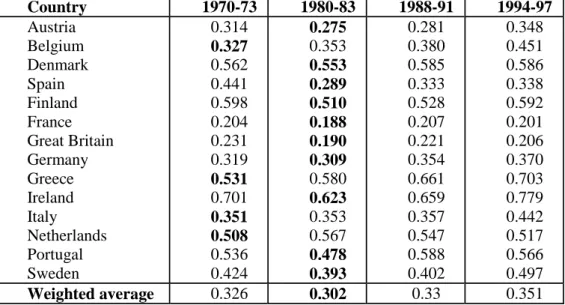
Table 2: Specialisation patterns in the EU

Country 1970-73 1980-83 1988-91 1994-97 Austria Belgium Denmark Spain Finland France Great Britain Germany Greece Ireland Italy Netherlands Portugal Sweden 0.314 0.327 0.562 0.441 0.598 0.204 0.231 0.319 0.531 0.701 0.351 0.508 0.536 0.424 0.275 0.353 0.553 0.289 0.510 0.188 0.190 0.309 0.580 0.623 0.353 0.567 0.478 0.393 0.281 0.380 0.585 0.333 0.528 0.207 0.221 0.354 0.661 0.659 0.357 0.547 0.588 0.402 0.348 0.451 0.586 0.338 0.592 0.201 0.206 0.370 0.703 0.779 0.442 0.517 0.566 0.497 Weighted average 0.326 0.302 0.33 0.351

Note: Minimum values for each country in bold font. Calculations based on four year averages at the dates indicated.

Table 2, taken from Midelfart-Knarvik et al. (2002) reports Krugman specialisation coefficients for 14 EU countries based on data from the OECD STAN database for 36 industries covering the period 1970 to 1997. Minimum values for each country are highlighted in bold. From the table, it is clear that the UK and France are the least specialised of the EU 15 countries. For these two countries, only roughly 10% of industrial activity would have to switch industry to bring them in to line with the rest of the EU.18 Ireland and Greece are the most specialised. For Ireland, 39% of industrial activity would have to switch industry to bring it in to line. We can roughly identify four groups of countries in terms of specialisation patterns. The big core countries (France, Germany, and the UK) tend to be least specialised. Small core countries tend to be slightly more specialised (Austria, Belgium, the Netherlands). Scandinavian countries are more

18

The rest of the EU is calculated excluding the country in question (see our earlier discussion). The amount of industry that would have to move is calculated as the Krugman index divided by 2, because the measure counts both positive and negative deviations.

19 specialised still (Sweden, Denmark, Finland). Finally cohesion countries tend to be most specialised (Greece, Ireland and Portugal).19 Of course, these groups have fuzzy boundaries and overlap somewhat. Spain and Italy are outliers from this classification. Italy is a big core country with specialisation patterns roughly similar to the smaller core countries. Spain is a cohesion country with remarkably low levels of specialisation.

Further results from Midelfart-Knarvik et al. (2003) on bilateral comparisons and the type of industries in which a country specializes helps understand these differences. The French and UK economies are very similar to one another and quite similar to Germany. Of course, because of their size, any two of these countries have a heavy weight when calculating the production structure for the rest of the EU and this tends to reduce the specialisation measures. All three countries tend to specialise in high tech, high skill industries. In contrast, France, the UK and Germany are most dissimilar to Greece and Ireland and fairly dissimilar to Portugal explaining the high specialisation of these three countries. The least specialised of the cohesion countries, Spain, is relatively similar to the big three. In terms of the types of industries in which the Cohesion four are specialising, Ireland is the clear outlier. Greece and Portugal are tending to specialise in low tech, low skill industries, Spain in medium tech, medium skill while Ireland has focused on high tech, high skill industry. Patterns in terms of the other two groups are also mixed. Of the three small core countries, Austria and Belgium are fairly similar in terms of both production structure and the type of industry (medium skill, medium tech). The Netherlands is the outlier of that group, both in terms of production structure and the type of industry (higher skill, but lower tech). Amongst the Scandinavian’s Finland and Sweden have similar production structures although Sweden’s is slightly higher tech. Denmark’s production structure is quite different to both these countries focusing on industries that are medium skill and medium tech making it more similar to Austria and Belgium. The reader is referred to Midelfart-Knarvik et al. (2003) for more details.

Once we turn to changes in specialisation, we can draw on a wider literature. In an early paper, Helg et al. (1995) present specialisation figures for the EU 12 countries based on the OECD Indicators for Industrial Activity for eight, 1-digit ISIC industries. Their results suggest that all countries, except France, Portugal and Spain become more specialised between 1975 and 1995. Their results are hard to interpret however as they are purely based on the shares of output of each industry in each country. Changes in the composition of output that are common across EU countries (say a move from textiles in to chemicals) will show up as increased specialisation. Thus, these numbers capture both the change in individual countries relative to the rest of the EU and the change in the EU relative to the rest of the world. More recent studies have tended to focus on shifts in countries specialisation patterns relative to the rest of the EU as the key variable of interest. Amiti (1999), Brülhart (1998a,b, 2001a,b), Brülhart and Torstensson

19

The “Cohesion countries” is often used to describe the four poorest members of the EU15: Greece, Ireland, Portugal and Spain. The name reflects the fact that all four receive Cohesion Fund money from the EU aimed at increasing economic convergence with the rest of the EU.

20 (1996), CEPII (1997), OECD (1999), WIFO (1999) Midelfart-Knarvik et al. (2002, 2003) and Storper et al. (2002) all present results on specialisation for EU nations. Some differences arise due to differences in data, time periods and measurement techniques. However, the results from Midelfart-Knarvik et al. (2002) reported in Table 2 tell the basic story. Most countries were least specialised at the beginning of the 1980s, although four countries had already reached their minimum in the 1970s. Subsequent changes led all countries to become more specialised. Findings from WIFO (1999) using the more detailed industrial classification available for the DAISIE database are similar (although the exact timings differ slightly). Midelfart-Knarvik et al. (2003) also report bilateral comparisons using the same data. Of 91 distinct pairs, 71 exhibit increasing difference between the early 1980s and the 1990s.

Our feeling is that this sort of study has now hit fairly rapidly decreasing returns. As outlined in Section 3.1 attempts to collapse the entire structure of industrial production down to one number that can be compared across time and across countries are fraught with many difficulties and these studies suffer from a number of problems. These descriptive pieces epitomize the area based approach we discussed in the introduction. They are useful for generating some stylised facts about location and integration in the EU, but they can tell us very little about what is causing those patterns or about location theory more generally. To summarize the key stylised finding that does emerge – the degree of specialisation varies substantially across the EU and the bulk of the evidence suggests that EU countries are slowly becoming more specialized.

2.2.3. A mixed picture for regional specialisation

Following our discussion in Section 1, it should be clear that data availability means making statements about economic activity in the EU at the regional level is much more difficult than making comparisons at the country level. Again, individual country studies exist, for example Smith (1975) for the UK, or Paluzie et al. (2001) for Spain, but there are relatively few studies taking an EU wide perspective.

Molle (1997) provides the longest historical perspective that we can find. He reports Krugman coefficients of specialisation for 96 EU regions providing figures every 10 years from 1950 to 1990. Data limitations mean that he considers NUTS 2 regions for France, Spain and Italy, NUTS 1 regions for the UK and Germany, and country data for Sweden, Finland, Denmark, Ireland, Portugal and Greece.20 He identifies three groups of regions. The overwhelming majority saw specialisation fall continuously throughout the period. A much smaller number saw a small rise in the 1950s, but a fall since. Finally, another small group saw no change, but these regions tended to have low specialisation coefficients to begin with. This is hardly the mixed picture to which the title of this subsection alludes. However, on close inspection, the numbers turn out to be quite hard to interpret. The calculations are based on

20

21 Eurostat’s NACE 17 industrial classification dividing employment in to 17 branches. As we saw in Section 1 six of these branches cover service sectors. Of these service branches, five are market service branches and a sixth is non-market services. Between them these service sectors count for nearly 70% of employment by 1990. Arguably, the composition effects from the growth in services21, the tendency for some of the services (such as catering) to closely mirror population, the non-market nature of non-market services, and the rather aggregate regional classification mean that any changes in specialisation patterns are likely to be obscured. More recent work suggests that all of these concerns may be relevant.

Hallet (2000) suggests that even small increases in the number of regions tend to give a more mixed picture. Using the same NACE 17 industrial classification, but 119 regions instead of 96, he finds that between 1980 and 1995, 34 regions became more specialised, while 85 regions became less specialised. In contrast to Molle (1997), Hallet (2000) does discuss the fact that the changing composition of output from industry (where the NACE 17 classification is finer) to services (where it is more aggregate) will artificially reduce measures of specialisation, but does not then present figures just for the nine industrial branches. Midelfart-Knarvik and Overman (2002) do just that. Just focusing on industrial branches, they find a much more mixed picture. Now, a majority of regions (53%) become more specialised, with the remainder showing either a decrease or no change. On average, however, increases in regional specialisation are small.

Given the problems with EU data at the regional level, it could be useful to look at individual country data to get a richer picture. Unfortunately, these papers usually suffer from all the same problems as the EU wide papers and are nearly always written from a national perspective. To take a good example, Paluzie et al. (2001) consider specialisation for 50 Spanish provinces (NUTS 3) for 30 manufacturing sectors over the time period 1979-1992. They find that 16 out of the 50 provinces show very small increases in specialisation while the rest show moderate decreases in specialisation. However, results from Table 2 suggest that Spain became more specialised relative to other EU countries. So, the fact that Spanish regions did not change much with respect to one another does not mean that Spanish regions did not become more specialised relative to the rest of the EU. Of course, which of these questions is more interesting may well depend on the theoretical model that you have in mind (C7). This brief discussion also suggests decomposing changes in to within and between nations although we do not know of any study that does this.

All of this suggests the need for considerable caution in reaching conclusions at the regional level. Problems with getting regional data, composition effects and the lack of good detailed disaggregate data makes it difficult to reach broad conclusions for the EU’s regions. The pattern appears mixed, but it is

21 _{The classification for industrial activity is much finer relative to the overall industrial employment than the classification for} services (9 industrial classifications to cover 30% of employment versus 6 industrial classifications to cover 70%). Thus as activity switches from several manufacturing branches in to fewer service branches we get a statistical reduction in specialisation.

22 clear that more careful analysis and better data seem to be pushing us in the direction of finding slightly more regional specialisation than we initially thought.

2.2.4. A mixed pattern for industrial concentration

Overall manufacturing activity is concentrated in the four biggest countries of the EU. In the mid 1990s Germany accounted for roughly 30% of total output, France 15%, Italy 14.5% and the UK 14%. Patterns in terms of overall manufacturing share are remarkably stable between 1970 and the mid-1990s at the national level. France and the UK have been the biggest losers with roughly a 2 and 3 percentage point decline respectively. Italy has been the biggest gainer, increasing its share from 12.5% to 14.5% (Midelfart-Knarvik et al., 2003). The picture is different at the regional level where overall concentration (as measured by the coefficient of variation) has increased considerably, at least from 1980 onwards.

As for regional specialisation, when we turn to looking at the distribution of individual industries across locations the pattern is again mixed. There are marked differences across industries in the degree to which they are concentrated. In terms of changes over time, some industries are becoming increasingly geographically concentrated, others are becoming less concentrated. We first deal briefly with the changes over time, before considering the characteristics of spatially concentrated industries in some detail in section 2.2.5.

Midelfart-Knarvik et al. (2003) use production data from the OECD STAN database to calculate absolute Gini coefficients of concentration for 36 manufacturing sectors based on four year averages (1970-73, 1980-83, 1990-93, and 1994-97). They find that concentration is increasing for 12 industries and decreasing for the remaining 24 industries. There is considerable variation over time. In the 1970s, 11 industries became increasingly concentrated, while 25 became less so. This pattern was reversed in the 1980s, with increasing concentration the norm (23 industries relative to 13 industries) before reversing again in the 1990s (15 industries increasing relative to 21). Table 3 shows the Gini coefficients for the 1970s, the 1990s and the change between those two periods. The industries are sorted from most to least concentrated according to how concentrated they were in the 1990s. The results broadly agree with those of Amiti (1999) using UNIDO production data for 27 manufacturing sectors for 10 EU countries.22

22 _{They differ somewhat from Brülhart (2001a) who conducts a similar exercise using employment data for 12 of the EU 15} countries. Brülhart's results are hard to interpret, however. First, he excludes Belgium, Ireland and Luxembourg due to data availability. Second, he fails to time average the data, instead presenting the change between 1996 and 1972. It is thus difficult to know whether his findings are driven by structural differences, or just differences in the business cycle across countries.

23

Table 3: Industrial concentration across EU countries

Industry Gini Change Industry Gini Change

Motor Vehicles 0.703 0.009 Furniture & Fixtures 0.596 0.028 Pottery & China 0.695 0.071 Machinery & Equipment nec 0.592 -0.071

Aircraft 0.693 0.016 Tobacco 0.592 -0.07

Leather & Products 0.685 0.138 Railroad Equipment 0.591 -0.048 Petroleum & Coal Products 0.682 0.009 Communication equipment 0.589 -0.065 Motorcycles & Bicycles 0.671 0.029 Glass & Products 0.569 -0.047

Footwear 0.669 0.075 Metal Products 0.567 -0.009

Electrical Apparatus nec 0.645 -0.023 Textiles 0.566 0.012

Transport Equipment nec 0.628 0.077 Beverages 0.557 -0.09

Rubber Products 0.624 0.005 Other Manufacturing 0.552 -0.025 Non-Ferrous Metals 0.623 0.042 Industrial Chemicals 0.546 -0.067 Chemical Products nec 0.622 -0.036 Non-Metallic minerals nec 0.542 -0.034 Petroleum refineries 0.621 -0.01 Pharmaceuticals 0.519 -0.078 Wearing Apparel 0.613 0.038 Printing & Publishing 0.515 -0.024

Iron & Steel 0.611 -0.014 Wood Products 0.498 -0.035

Office & Computing Machinery 0.608 -0.072 Paper & Products 0.479 -0.025

Plastic Products 0.6 -0.002 Food 0.46 -0.043

Professional Instruments 0.597 -0.068 Shipbuilding & Repairing 0.445 -0.022

Turning to the regional level, we are again hampered by data availability. As for specialisation, Molle (1997) provides the longest historical study we can find looking at changes in industrial concentration from 1950 to 1990. The paper uses the Krugman index of concentration. The data and regional definition are the same as for his study of regional specialisation. The results show that most sectors experience a decrease in concentration. Only Agriculture and Textiles show an increase, while Mining, and Food, Beverages and Tobacco show no clear pattern. However, as for specialisation, the inclusion of service sectors makes the results very hard to interpret due to the compositional changes over the time period. To see the problem, consider one particular manufacturing sector such as transport equipment. Imagine that, relative to manufacturing the concentration of transport equipment remained unchanged. What happens to the index will now be driven purely by the relationship between changes in regional manufacturing shares and changes in shares in other activities. Again, whether this makes sense will depend on the null hypothesis (C3) and theory (C7) one has in mind.

We have little additional evidence. In a recent paper, Brülhart and Traeger (2002) consider changes in regional specialisation using data for NUTS 2 regions disaggregating employment in to eight sectors covering the full range of economic activities. They decompose concentration in to what they call topographic and relative components. Topographic concentration considers the degree to which sectors are concentrated in geographical space, relative concentration the degree to which sectors are concentrated relative to overall activity. Although preliminary, their results suggest that the topographic distribution of total employment is stable. Broad sectors show conflicting movements, with agriculture becoming more topographically concentrated and manufacturing less. For individual sectors however, only transport and communication services and non-market services show significant decreases, while the

24 four remaining sectors remain unchanged. This overall stability is increasingly driven by between country considerations rather than within country considerations. Turning to relative concentration, they find that there has been a monotonic increase in the relative concentration of manufacturing. Further, their evidence suggests that these increases are significant. In contrast, Transport and communications and Non-market services have seen significant reductions in their relative concentration.

2.2.5. The characteristics of spatially concentrated industries

In the introduction, we suggested that in an ideal world, this chapter would need to do two things. First, spend a lot of time describing the location of economic activity in the EU. Second, explain these patterns drawing widely on other chapters in the handbook, leaving us to consider in depth only material that helps us understand why things in the EU might be different. Obviously, this second stage would require us to clearly identify the differences between the EU and the US. Data quality and conceptual issues mean this has proved difficult to do, so the literature has taken a different route. This area-based descriptive work has now spawned a new set of area-based explanatory pieces using methodologies that allow for the limited amount of data available in the EU.

In this section we consider the characteristics of concentrated industries by looking at what we think of as this “first generation” of area-based studies. These follow Kim (1995) in examining the determinants of concentration by considering the correlation between spatial concentration and industry characteristics. We review this literature in depth here. We conclude that, for a number of reasons, this work often ends up telling us very little about what explains the economic geography of Europe. While the authors often claim that these papers represent tests of various economic geography models, we believe that they are purely descriptive in nature.

Two early papers, Brülhart and Torstensson (1996) and Brülhart (1998b) use employment data to compute rank correlations between Gini indices of spatial concentration and returns to scale and to consider whether concentrated industries are found in core or peripheral locations. They do this for two years, 1980 and 1990, for 11 countries (EU 12 minus Luxembourg) and 18 manufacturing industries. Data is from EUROSTAT and the OECD. Returns to scale are based on Pratten (1988). Core and peripheral locations are defined using a simple market potential based on GDP and geodesic distances. Brülhart (1998b) extends this work by further classifying industries according to their labour and resource intensity, whether they are science based, and whether goods are highly differentiated. His classification is taken from OECD (1987). Both papers also study the impact of these determinants on intra-industry trade using a Grubel-Lloyd index for six points between 1961 and 1990.

In contrast to Kim (1995), neither paper uses time varying explanatory factors ruling out the use of industry fixed effects. This is unfortunate as industry fixed effects could control for some of the problems with both the concentration measure and the explanatory variables. In particular, in line with the discussion of C3 in Section 2.2.1, fixed effects can partly account for the fact that the Gini index