Kelvin Waves in the Nonlinear Shallow Water Equations on the Sphere: Nonlinear Traveling Waves and the Corner Wave Bifurcation

Kelvin Waves in the Nonlinear Shallow Water Equations on the Sphere: Nonlinear Traveling Waves

and the Corner Wave Bifurcation

John P. Boyd Cheng Zhou

University of Michigan

Two Topics

1. New asymptotic approximation for LINEAR Kelvin waves on the sphere

2. Corner wave bifurcation for NONLINEAR Kelvin waves on the sphere

Restrictions

1. Nonlinear shallow water equations 2. No mean currents

Two Parameters

1. Integer zonal wavenumber s s > 0

2. Lamb’s Parameter ≡ 4Ω2a2 gH

Ω = 2π/84, 600 s, a = earth’s radius

Parametric range is SEMI-INFINITE in BOTH

s &

Table 1: Lamb’s Parameter

Description Source

0.012 External mode: Venus Lindzen (1970) 6.5 External mode: Mars Zurek (1976) 12.0 External mode: Earth (7.5 km equivalent depth) Lindzen (1970)

2.6 Jupiter: simulate Galileo data Williams (1996)

21.5 Jupiter Williams (1996)

43.0 Jupiter Williams (1996)

260 Jupiter Williams (1996)

2600 Jupiter Williams and Wilson (1988) 87,000 ocean: first baroclinic mode (1 m equiv. depth) Moore & Philander (1977) >100,000 ocean: higher baroclinic modes Moore & Philander (1977)

LINEAR EIGENFUNCTIONS are

“HOUGH” functions (S. S. Hough (1896, 1898)

“We regard Mr. Hough’s work as the most important contribution to the dynamical theory of the the tides since the time of Laplace.”

Kelvin Parameter Space & LINEAR Asymptotic Regimes

Small : u = P_ss(cos(θ)) exp(isλ − iσt) (Longuet-Higgins, 1968))

Large : u ∼ exp(−√θ2) exp(isλ − iσt)

√

_

ε

? ?

?

?

?

?

?

?

?

?

?

?

New asymptotic approximation is (µ = sin(latitude))

φ ≈ (1 − µ2)s/2 exp(−(1/2) + s2 − s

µ2) Approximation (thick solid curve) and exact (thin solid curve) are GRAPHICALLY

INDIS-TINGUISHABLE for s = 5, = 5 0.3 0.4 0.5 0.6 0.7 0.8 0.9 ε =5 s=5 φ

Uniform Validity

• New approximation is uniformly valid for

s2 + >> 1 (shaded in figure)

• Though not strictly valid when both s and

are O(1), it is not a bad approximations

√

_

ε

Barotropic ( = 0) Kelvin Waves Equatorial trapping is not just due to

High zonal wavenumber Kelvin are equatorial

modes even for = 0

Barotropic ( = 0) Kelvin Waves Half-width is inside the tropics for s ≥ 5

-900 -60 -30 0 30 60 90 0.2 0.4 0.6 0.8 1 colatitude

Barotropic Kelvin waves: s=1, 2, ..., 10

u or

φ

s=1 _{s=10 s=10 s=1}

Weakly Nonlinear Wave Theory, A Science Fiction Story

• Perturbative theory yields approximations that have the structure of LINEAR Kelvin waves in LATITUDE & DEPTH multiplied by a function A(x, t) that solves a nonlinear PDE

u = h = A(x, t) exp(−0.5y2)φ(z); v ≡ 0

• On equatorial beta-plane without currents, Kelvin is dispersionless:

A_t + A_x + 1.22 AA_x = 0 [1D Advection Eq] (1)

• Breaking and frontogenesis; no steady propagation

velocity scale is about 2 m/s length scale is about 300 km

Kelvin Fronts & Breaking Boyd (J. Phys. Oceangr., 1980) Ripa (J. Phys. Oceangr., 1980)

Front curvature due to Kelvin-gravity wave resonance

Boyd (Dyn. Atmos. Oceans, 1998)

Fedorov & Melville (J. Phys. Oceangr., 2001) Microbreaking

Boyd (Phys. Lett. A, 2005)

-3 -2 -1 0 1 2 3 -1 -0.5 0 0.5 1 x A A_t + A A_x = (1/100) A_xx, A(x,0)= - sin(x)

Shear Currents: Dispersion

• Equatorial ocean has strong currents:

South Equatorial Current (westward), North Equatorial Countercurrent (eastward), etc.

• Currents induce dispersion in Kelvin wave

• (Boyd, Dyn. Atmos. Oceans, 1984)

A_t + 1.22 AA_x + dA_xxx = 0[KdV Eq] KdV Predictions:

1. Solitons & cnoidal waves of

arbitrarily large amplitude

Difficulties with KdV Picture for Kelvin Wave

• KdV dispersion relation predicts a PARABOLA

for the group velocity: true for k < 1 only

• As k → ∞, c_g → c_phase → constant

• Kelvin is WEAKLY DISPERSIVE for large

zonal wavenumber (Boyd, JPO, 2005)

• KdV Theory FAILS at LARGE AMPLITUDE

because shear-induced dispersion is TOO WEAK to balance NONLINEAR STEEPENING

0 1 2 3 4 0.95 1 1.05 1.1 1.15 1.2

Kelvin group velocity in shear flow

zonal wavenumber k asymptotically flat e xt_ra p o la ted K d V d is_p er s io_n

Solitons on the Union Canal

Solitary waves were discovered observationally by John Scott Russell in the 1830’s. Below is a modern recreation on the same canal.

What Really Happens: CCB Scenario Amplitude Cnoidal Breaking CCB Scenario: Cnoidal/Corner/Breaking Corner

Nonlinear Kelvin Waves on the Sphere (Boyd and Zhou, J. Fluid Mech., 2009)

• NO SHEAR: ALL DISPERSION from

SPHERICAL GEOMETRY

• Small amplitude/small double perturbation series

• Spectral-Galerkin model

• Newton/continuation

• Kepler change-of-coordinate to resolve the dis-continuous slope of the corner wave

• Zoom plots to identify the corner wave as tallest, non-wiggly solution

• Cnoidal/Corner/Breaking Scenario: All waves

above an -dependent maximum amplitude

break, as confirmed by initial-value time-dependent computations.

Kelvin Wave on the Sphere-2

With no mean currents, corner wave occurs

at SMALLER and SMALLER amplitude as

increases

On the equatorial beta-plane ( = ∞), ALL KELVIN WAVES BREAK

10−2 10−1 100 101 10−2

10−1 100

φ₀₀ in the corner wave limit

ε

φ 00

s=1 s=2

Figure 4: Maximum ofφ(x, y) for the corner wave versus. The maximum always occurs at the crest of the wave (X = 0) and right at the equator (y= 0).

φ₀₀ is the height at the peak, x = 0 and y = 0

Kelvin Wave on the Sphere-3

As decreases, the corner wave profile

be-comes narrower and narrower in longitude — more soliton-like. −1.5 −1 −0.5 0 0.5 1 1.5 −0.4 −0.2 0 0.2 0.4 0.6 0.8 1 φ(x,y=0) normalized by φ 00 s=2 Longitude φ (x,y=0) ε=0.01 ε=1 ε=5 ε=30

Figure 5: An equatorial cross-section of the height/pressure fieldφ,φ(x, y= 0), for several, normalized by φ(0,0).

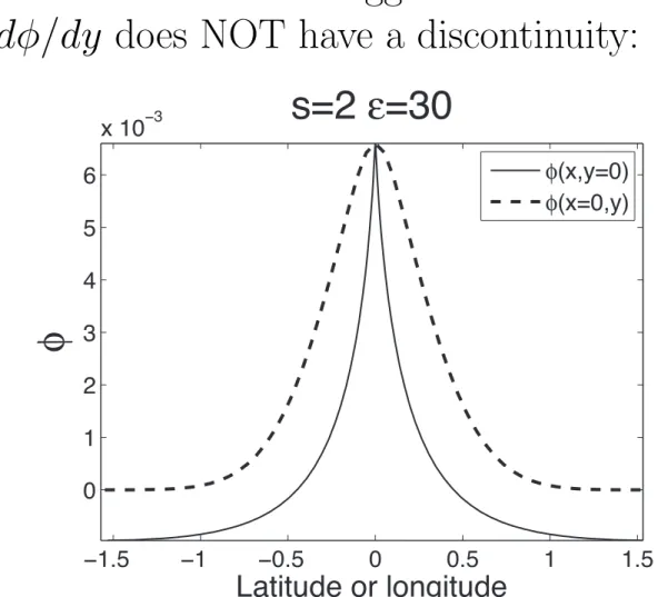
Kelvin Wave on the Sphere-4

CONE, CREASE or ONE-SIDED POINT SINGULARITY?

Numerical evidence suggests the latter

dφ/dy does NOT have a discontinuity:

−1.5 −1 −0.5 0 0.5 1 1.5 0 1 2 3 4 5 6 x 10−3 Latitude or longitude φ s=2 ε=30 φ(x,y=0) φ(x=0,y)

Kelvin Wave on the Sphere-5

Two views of the same corner wave below:

−2 0 2 −1 0 1 −0.05 0 0.05 0.1 0.15

s=1

ε

=1

φ

=

0.1905

Kelvin Wave on the Sphere-6

dφ/dx has a JUMP DISCONTINUITY at the EQUATOR ONLLY

(Insofar as one can judge singularities from nu-merical computations.) −1 −0.5 0 0.5 1 1.5 −5 0 5 Longitude φ_x s=2 ε=0.01 lat=0 lat=π/64 lat=π/32 lat=π/16 lat=π/8 lat=π/4 −0.1 −0.05 0 0.05 0.1 −5 0 5 Longitude φ_x lat=0 lat=π/64 lat=π/32 lat=π/16 lat=π/8 lat=π/4

Figure 7: dφ/dx fors= 2 and= 1/100. The right panel is a “zoom” plot of the left panel, showing only 1/15 the range in longitude.

Summary

After 35 years of intermittent studies of the Kelvin wave and one thesis chapter and 14 arti-cles (out of 195) from 1976 to present, still are

UNRESOLVED QUESTIONS

• Why does the travelling wave branch, for Kelvin and so many other wave species, terminate in a corner wave?

• Complete classification of generic & non-generic features in corner wave bifuraction.

• How does microbreaking promote mixing in

the ocean?

• How does nonlinearity reshape the Kelvin mode’s role in El Ni´no?

• Does the breaking Kelvin wave overturn or stay single-valued?

“Before I came here I was confused about this subject. Having listened to your lecture I am still confused, but on a higher level.”

Equatorial Beta-Plane: → ∞ limit of tidal equations

• Sines & cosines of latitude ⇒ y and 1.

• Hough functions become Hermite functions

(v, or sums of two Hermite functions (u, φ).

• Tropical is well-approximated, even NONLIN-EAR, by “one-and-a-half-layer” model

• Linear dynamics is beta-plane form Laplace’s Tidal Equations with actual depth of upper layer (average: 100 m) replaced by equivalent depth (0.4 m).

Warm, Light, Moving Layer

Cold, Heavy, Infinitely Deep Motionless Layer

• Kelvin & Rossby waves are disturbances on the “main thermocline”, which is the inter-face between the warm layer and the cold layer.

• Approximation is not too bad for ocean.

• In one-and-a-half-layer model, wave is only a function of latitude y and longitude x and time t.

Soliton-Machine at Snibston Discovery Park (England)

Recreating solitons in a channel is literally child’s play.

Kelvin Solitary Waves

• Initial-value numerical solutions of shallow wa-ter equations confirm solitons in a shear flow.

-10 0 10 0 0.05 0.1 u: Kelvin mode t=0 & t=100 -10 0 10 -0.05 0 0.05 x

du/dx: Kelvin mode

0 2 4 6 -0.5

0 0.5 1

Mean wind & height

-2 0 2 0 2 4 6 x y Kelvin soliton at t=100 U Φ

Figure 10: KELVIN SOLITON: left panels: Initial and final amplitude of the Kelvin mode. Upper right: mean flow & height. Lower right: contours of pressure/height and vector arrows. u(x, y,0) =φ(x, y,0) = 0.12sech2(0.7x)−constant.

“Planetary Waves and the Semiannual Wind Oscillation in the Tropical Upper Stratosphere,” Ph. D. Thesis, Harvard (1976)

5. ”The Effects of Latitudinal Shear on Equatorial Waves, Part I: Theory and Methods,” J. Atmos. Sci., 35, 2236-2258 (1978).

6. ”The Effects of Latitudinal Shear on Equatorial Waves, Part II: Applications to the Atmosphere,” J. Atmos. Sci., 35, 2259-2267 (1978).

7. ”The Nonlinear Equatorial Kelvin Wave,” J. Phys. Oceangr., 10, 1-11 (1980).

18. ”Low Wavenumber Instability on the Equatorial Beta-Plane,” with Z. D. Christidis, Geophys. Res. Lett., 9, 769-772 (1982).

22. ”Instability on the Equatorial Beta-Plane,” with Z. D. Christidis, in Hydrodynamics of the Equatorial Ocean, ed. by J. Nihoul, Elsevier, Amsterdam, 339-351 (1983).

25. ”Equatorial Solitary Waves, Part 4: Kelvin Solitons in a Shear Flow,” Dyn. Atmos. Oceans, 8, 173-184 (1984).

60. ”Nonlinear equatorial Waves”. In Nonlinear Topics of Ocean Physics, Proceedings of the Fermi Summer School, Course 109, ed. by A. R. Osborne and L. Bergamasco. North-Holland, Amsterdam, 51-97 (1991).

98. ”High Order Models for the Nonlinear Shallow Water Wave Equations on the Equatorial Beta-plane with Application to Kelvin Wave Frontogenesis”, Dyn. Atmos. Oceans., 28, no. 2, 69-91 (1998)

106. ”A Sturm-Liouville Eigenproblem of the Fourth Kind: A Critical Latitude with Equatorial Trap-ping”, with A. Natarov, Stud. Appl. Math., 101, 433-455 (1998).

110. ”Propagation of Nonlinear Kelvin Wave Packet in the Equatorial Ocean”, with G.-Y. Chen, Geophys. Astrophys. Fluid Dynamics., 96, no. 5, 357-379 (2002).

115. ”Beyond-all-orders Instability in the Equatorial Kelvin Wave”, with Andrei Natarov, Dyn. Atmos. Oceans., 33, no. 3, 181-200 (2001).

118. ”Shafer (Hermite-Pade) Approximants for Functions with Exponentially Small Imaginary Part with Application to Equatorial Waves with Critical Latitude” with Andrei Natarov, Appl. Math. Comput., 125, 109-117 (2002).

138. ” Fourier Pseudospectral Method with Kepler Mapping for Travelling Waves with Discontinuous Slope: Application to Corner Waves of the Ostrovsky-Hunter Equation and Equatorial Kelvin Waves in the Four-Mode Approximation, Appl. Math. Comput. , 177, no. 1, 289-299(2006).

146. ”The Short-Wave Limit of Linear Equatorial Kelvin Waves in a Shear Flow”, J. Phys. Oceangr., 35, no. 6 (June), 1138-1142. (2005).