Bounded-variable least-squares methods for linear and nonlinear model predictive control

(1)

IMT School for Advanced Studies Lucca

Lucca, Italy

Bounded-Variable Least-Squares Methods for

Linear and Nonlinear Model Predictive Control

PhD Program in Computer Science and Systems

Engineering

XXXI Cycle

By

Nilay Saraf

(2)

(3)

The dissertation of Nilay Saraf is approved.

Program Coordinator: Prof. Alberto Bemporad, IMT School for Advanced Studies Lucca, Italy

Supervisor: Prof. Alberto Bemporad,

IMT School for Advanced Studies Lucca, Italy

Co-supervisor: Dr. Daniele Bernardini, ODYS Srl

The dissertation of Nilay Saraf has been reviewed by:

Prof. Eric Kerrigan,

Imperial College London, UK

Prof. Ilya Kolmanovsky,

University of Michigan, Ann Arbor, MI

IMT School for Advanced Studies Lucca

2019

(4)

(5)

(6)

(7)

List of Figures

2.1 Mass-spring-damper system. . . 17 2.2 Closed-loop simulation of mass-spring-damper system:

controller performance. . . 18 2.3 Maximum perturbation introduced in the linear dynamics

as a function of the penaltyρ. . . 19 2.4 Value of slack variable on solving the soft constrained

problem (2.11) and violation of the equality constraint (2.10) at each time step. . . 20 2.5 Closed-loop simulation of mass-spring-damper system

with soft-constrained MPC and BVLS formulations. . . 21 2.6 Simulation results of the AFTI-F16 aircraft control

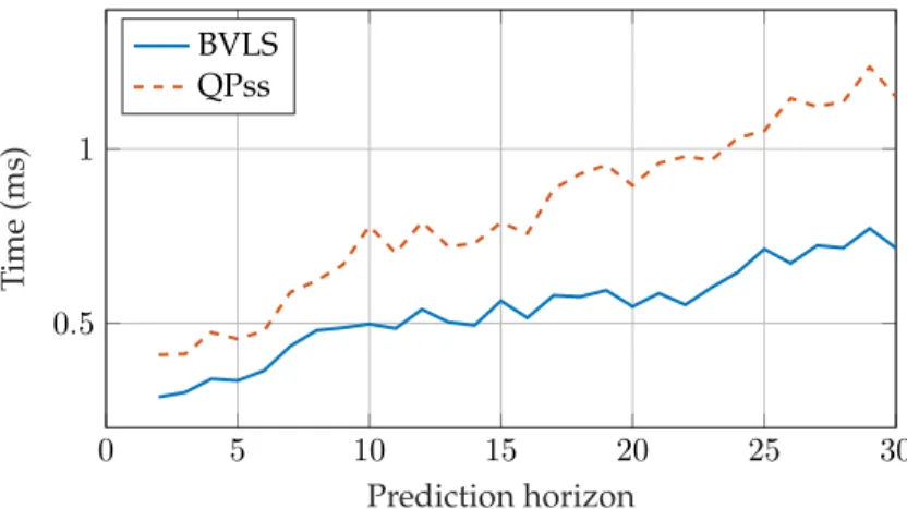
prob-lem: Worst-case CPU time to solve the BVLS problem based on I/O model and condensed QP (QPss) based on state-space model. . . 29 2.7 Simulation results of the AFTI-F16 aircraft control

prob-lem: Comparison of the CPU time required to construct the MPC problems (2.9) and (2.26a) against prediction ho-rizon. . . 30 2.8 Simulation results of the AFTI-F16 aircraft control

prob-lem: Comparison of the worst-case CPU time required to update the MPC problem before passing to the solver at each step. . . 30

(11)

3.1 Performance in tracking and regulation using formula-tion (3.8). . . 42 3.2 Comparison of the optimized cost for the problem

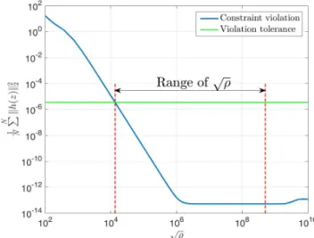
formu-lations (3.6), (3.8). . . 43 3.3 Equality constraint violations versusρfor NMPC of CSTR

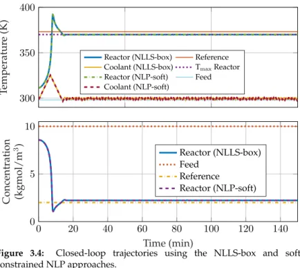
simulations in double precision floating-point arithmetic1_. Duration of each simulation was 1500 steps of 6 seconds. . 44 3.4 Closed-loop trajectories using the NLLS-box and

soft-constrained NLP approaches. . . 46 3.5 Constraint relaxation comparison between the NLLS-box

and soft-constrained NLP approaches. . . 47 4.1 Solver performance comparison for BVLS test problems

with condition number of matrix A = 108_{, 180 random}

instances for eachA∈R1.5n×n, and all possible non-zero cardinality values of the optimal active set. . . 67 4.2 Solver performance comparison for BVLS test problems

with condition number of matrix A = 108_{: comparison}

of cost function values. . . 68 4.3 Solver performance comparison for BVLS formulation

based tracking-MPC simulation of AFTI-F16 aircraft. . . . 71 4.4 Comparison of the performance (solver time) of

QPoases C with BVLS (2.9) and condensed QP (2.26a) formulations for the AFTI-F16 LTI MPC problem. . . 72 4.5 Modicon M340 PLC of Schneider Electric used for the

hardware-in-the-loop tests. . . 73 4.6 Quadruple tank system. . . 74 4.7 Closed-loop trajectories of I/O variables during tracking

MPC of the quadruple tank system using PLC. . . 77 4.8 Closed-loop trajectories of the quadruple tank system’s

I/O variables during disturbance rejection tests using RB-VLS based MPC on PLC. . . 78

(12)

4.9 Solver performance comparison for BVLS test problems with condition number of matrix A = 104_{, 180 random}

instances for eachA∈R1.5n×n, and all possible non-zero cardinality values of the optimal active set. . . 83 4.10 Solver performance comparison for BVLS test problems

with condition number of matrix A = 104_{: comparison}

of cost function values. . . 84 4.11 Solver performance comparison for BVLS test problems

with condition number of matrix A = 10, 180 random instances for eachA∈_R1.5n×n_{, and all possible non-zero} cardinality values of the optimal active set. . . 85 4.12 Solver performance comparison for BVLS test problems

with condition number of matrixA = 10: comparison of cost function values. . . 86 4.13 Number of iterations of each solver while solving the

ran-dom BVLS test problems with condition number of matrix A= 108_{, referring the comparision in Figure}_4.1_{. . . .} ₈₇

4.14 Number of iterations of each solver while solving the ran-dom BVLS test problems with condition number of matrix A= 104, referring the comparision in Figure4.9. . . 88 4.15 Number of iterations of each solver while solving the

ran-dom BVLS test problems with condition number of matrix A= 10, referring the comparision in Figure4.11. . . 89 5.1 CPU time for each solver during closed-loop simulation of

the CSTR w.r.t. prediction horizon. . . 100 6.1 Sparsity pattern of equality constraint Jacobian Jhk for a

random model with Np = 10, Nu = 4,na = 2,nb = 4,

nu= 2andny = 2. . . 107 6.2 Sparsity pattern of JacobianJ and its thin QR factors,

re-ferring (6.6), (6.5), for a random NARX model with non-zero coefficients, diagonal tuning weights, and parameters ny = 2,nu= 2,na= 2,nb= 1,Np= 4,Nu= 3. . . 116

(13)

6.3 Illustration showing changes in sparsity pattern of JF formed from columns of the Jacobian matrix J in Fig-ure6.2a, and its thin QR factors when an index is removed from the setF. . . 119 6.4 Illustration showing changes in sparsity pattern of JF

formed from columns of the Jacobian matrix J in Fig-ure 6.2a, and its thin QR factors (obtained without reor-thogonalization) when an index is inserted in the setF. . . 120 6.5 Computational time spent by each solver during NMPC

simulation of CSTR for increasing values of predictino ho-rizon. . . 123 6.6 Computational time spent by each solver during NMPC

(14)

List of Tables

4.1 Quadruple tank system parameters. . . 75 4.2 Operating point parameters for the quadruple tank system. 75

(15)

Acknowledgements

First of all, I would like to express my deepest gratitude to my advisor Prof. Alberto Bemporad who gave me a dream opportunity to work on my PhD at IMT. His wise ment-orship, profound expertise and an inspirational work ethic have all played a cruicial role in achieving the results of this thesis besides making a permanent positive impact on my personal and professional development. I sincerely thank my co-advisor Daniele Bernardini (ODYS) for his time and effort. During this long committment, timely meetings with him and Alberto always granted me the assurance and mo-tivation that I needed to push forward. I also thank Mario Zanon (IMT) for his effort and helpful discussions while we worked together on writing a paper. Next, I would like to sin-cerely thank Prof. Eric Kerrigan and Prof. Ilya Kolmanovsky for assessing the thesis and providing useful feedback. Thanks to all current and former members of the DYSCO re-search unit and study room, I enjoyed a friendly, pleasant and motivating work environment. I thank Vihang Naik, Manas Mejari, Sampath Mulagaleti, Ajay Sampathirao for all the discussions we had, and specially thank Laura Ferrarotti for carefully reviewing all math proofs, besides always being a caring friend. Personally, I would also like to express grat-itude to all my friends at IMT or away, oCPS fellows, former teachers, supervisors and colleagues. I thank all staff mem-bers at IMT and ODYS for their essential support throughout the last four years. It is a long list of people that I have not mentioned here but they know who they are and they will al-ways be remembered by me. Lastly and most importantly, I would like to thank my parents and sister for always being a

(16)

staunch support with unconditional love and care, which has been the cornerstone of all my successes.

I am grateful to the IMT school and the European commis-sion for supporting my PhD studies through the European Union’s Horizon 2020 Framework Programme for Research and Innovation under the Marie Skłodowska-Curie grant agreement No. 674875 (oCPS).

(17)

Vita

January 21, 1992 Born, Amalner, India

2009-2013 B.E. in Mechanical Engineering Final mark: Distinction

University of Mumbai, India

2013-2015 MSc. in Mechanical Engineering Specialization: Control Engineering Delft University of Technology, The Netherlands

10/14-04/15 Research Assistant (Masterand) Fraunhofer Institute for Solar Energy Systems, Freiburg, Germany

2015-2019 PhD Program in Computer Science and Systems Engineering

Research Unit: Dynamical Systems, Control, and Optimization

IMT School for Advanced Studies Lucca, Italy

(18)

Publications

1. N. Saraf and A. Bemporad, “Fast model predictive control based on linear input/output models and bounded-variable least squares,” inProc. 56th IEEE Conference on Decision and Control, Melbourne, Australia, 2017, pp. 1919 – 1924.

2. N. Saraf, M. Zanon, and A. Bemporad, “A fast NMPC approach based on bounded-variable nonlinear least squares,” inProc. 6th IFAC Conference on Nonlinear Model Predictive Control, Madison, WI, August 2018, pp. 337 – 342.

3. N. Saraf and A. Bemporad, “A bounded-variable least-squares solver based on stable QR updates,”IEEE Transactions on Automatic Control, 2019. [Online]. Available: https://ieeexplore.ieee.org/document/ 8747522

4. N. Saraf and A. Bemporad, “An efficient non-condensed approach for linear and nonlinear model predictive control with bounded variables,” in arXiv preprint arXiv:1908.07247, 2019. [Online]. Available: https: //arxiv.org/abs/1908.07247

(19)

Abstract

This dissertation presents an alternative approach to formu-late and solve optimization problems arising in real-time mo-del predictive control (MPC). First it has been shown that by using a quadratic penalty function, the linear MPC optim-ization problem can be formulated as a least-squares prob-lem subject to bounded variables while directly employing models in their input/output form. A theoretical analysis on stability and optimality is included with a comparison against the conventional condensed approach based on lin-ear state-space models. These concepts are straightforwardly extended for fast nonlinear MPC with bounded variables. An active-set algorithm based on a novel application of lin-ear algebra methods is proposed for efficiently solving the resulting box-constrained (nonlinear) least-squares problems with global convergence, numerical robustness, and easy de-ployability on industrial embedded hardware platforms. Fi-nally, new methods and tools are devised for maximizing efficiency of the solution algorithm considering the numer-ically sparse structure of the non-condensed MPC problem. Based on these methods, the problem construction phase in MPC design is systematically eliminated by parameterizing the optimization algorithm such that it can adapt to real-time changes in the model and tuning parameters while signific-antly reducing memory and computational complexity with a potentially self-contained matrix-free implementation. Nu-merical simulation results included in this thesis testify the potential, applicability, numerical robustness and efficiency of the proposed methods for practical real-time embedded MPC.

(20)

Chapter 1

Introduction

1.1 Motivation and research objectives

Model predictive control (MPC) is an advanced control method that is capable of controlling complex systems whose dynamical behaviour may be characterized by means of a mathematical model. Its ability to con-trol multivariable systems while handling constraints has made it one of the most popular methods in advanced control engineering practice with an ever growing range of applications in several industries. MPC evolved over the years from a method developed for controlling slow processes [1,2] to an advanced multivariable control method that is ap-plicable even to fast-sampling applications, such as in the automotive and aerospace domains [3,4]. This evolution has been possible because of the significant amount of research on computationally efficient real-time MPC algorithms. For an incomplete list of such efforts and tools the reader is referred to [5–9]. Despite the success of MPC, demand for faster numerical algorithms for a wider scope of applications has been reported for instance in [4]. A common approach to reducing computational load is to solve the MPC problem suboptimally, see for instance [5,9]. How-ever, even such MPC approaches have limitations that could be prohib-itive in some resource-constrained applications, especially in the case of (parameter-varying) nonlinear MPC (NMPC). This denotes that there is

(21)

still a large scope of improvement.

This thesis presents an alternative approach to formulate and solve optimization problems arising in real-time model predictive control. The proposed methods aim to stimulate the practical use of MPC in resource constrained applications. They are designed with the motivation to bridge the gap between MPC theory and industrial practice by taking into consideration that: data-based black-box models are often identified as difference equations in input/output (I/O) form; the control variables are often subject to simple bounds; numerically robust algorithms are re-quired for accuracy in limited precision computing which is common in embedded hardware platforms; an easy general deployment needs min-imization of calibration requirements; stand-alone code is required for embedded implementation. The main idea studied to meet these needs was to tailor the MPC problem formulation using penalty functions such that fast and simple optimization solvers can be employed. The resulting optimization problems can be solved using box-constrained (nonlinear) least-squares algorithms, which were researched in exhaustive detail.

1.2 Thesis outline and contributions

The thesis is structured into two parts: the first part (Chapters 2 -3) focuses on MPC problem formulations whereas the following part (Chapters4-6) focuses on optimization algorithms and their implement-ation. We refer to [10] for terminology and basic concepts about MPC. For details about constrained optimization algorithms and relevant ter-minology used in this thesis we refer to [11]. The content in this thesis is mainly based on the work published in [12–15]. First it has been shown how the linear MPC optimization problem can be formulated as a least-squares problem subject to bounded variables while directly employing models in their I/O form. A theoretical analysis on stability and optimality is included with a comparison against the conventional condensedapproach based on linear state-space models. These concepts are straightforwardly extended for fast nonlinear MPC. An active-set al-gorithm based on a novel application of linear algebra methods is

(22)

pro-posed for efficiently solving the resulting box-constrained (nonlinear) least squares problems with global convergence, numerical robustness, and easy deployability on industrial embedded hardware platforms. Fi-nally, new methods and tools are devised for maximizing efficiency of the solution algorithm considering the numerically sparse structure of the non-condensed MPC problem. Based on these methods, the problem construction phase in MPC design is systematically eliminated by para-meterizing the optimization algorithm such that it can adapt to real-time changes in the model and tuning parameters while significantly reducing memory and computational complexity with a potentially self-contained matrix-free implementation. Numerical simulation results included in this thesis testify the potential, applicability, numerical robustness and efficiency of the proposed methods.

The chapter-wise contribution is described in detail as follows

• Chapter 2, Fast model predictive control based on linear in-put/output models:

This chapter introduces a fast and simple model predictive control approach for multivariable discrete-time linear systems described by input/output models subject to bound constraints on inputs and outputs. The proposed method employs a relaxation of the dynamic equality constraints by means of a quadratic penalty func-tion so that the resulting real-time optimizafunc-tion becomes a (sparse), always feasible, bounded-variable least-squares (BVLS) problem. Conditions on the penalty parameter are derived for maintain-ing closed-loop stability when relaxmaintain-ing the dynamic equality con-straints. The approach is not only very simple to formulate, but also leads to a fast way of bothconstructing andsolvingthe MPC problem in real time, a feature that is especially attractive when the linear model changes on line, such as when the model is ob-tained by linearizing a nonlinear model, by evaluating a linear parameter-varying model, or by recursive system identification. A comparison with the conventional state-space based MPC ap-proach is shown in an example, demonstrating the effectiveness of

(23)

the proposed method. The content of this chapter is mostly based on [12].

• Chapter 3, Nonlinear model predictive control problem formula-tions:

In this chapter, we present an approach for real-time nonlinear model predictive control (NMPC) of constrained multivariable dy-namical systems described by nonlinear difference equations. The NMPC problem is formulated by means of a quadratic penalty function as an always feasible, sparse nonlinear least-squares prob-lem subject to box constraints on the decision variables. Linear time-invariant and linear time-varying model predictive control based on BVLS are special cases of the proposed NMPC frame-work. The proposed formulation and its benefits are demonstrated through a typical numerical example in simulation. An alternat-ive approach based on the augmented-Lagrangian method is also discussed. It is shown that inspite of fundamental differences with the former approach, the nonlinear non-convex optimization prob-lem in this case as well can be formulated to have exactly the same structure, which is favorable to employ fast solution methods. The content of this chapter includes excerpts from [13] and [15]. • Chapter4, Bounded-variable least-squares solver:

In this chapter, a numerically robust solver for least-squares prob-lems with bounded variables is presented for applications includ-ing, but not limited to, model predictive control. The proposed BVLS algorithm solves the problem efficiently by employing a re-cursive QR factorization method based on Gram-Schmidt ortho-gonalization. A reorthogonalization procedure that iteratively re-fines the QR factors provides numerical robustness for the de-scribed primal active-set method, which solves a system of linear equations in each of its iteration via recursive updates. The per-formance of the proposed BVLS solver, which is implemented in C without external software libraries, is compared in terms of compu-tational efficiency against state-of-the-art quadratic programming

(24)

solvers for small to medium-sized random BVLS problems and a typical example of embedded linear MPC application. The numer-ical tests demonstrate that the solver performs very well even when solving ill-conditioned problems in single precision floating-point arithmetic. Preliminary results in a hardware-in-the-loop setting based on BVLS-based MPC of a mildly nonlinear system with the proposed optimization solver embedded on a programmable lo-gic controller are included, which demonstrate the success of the methods in practically addressing key issues such as numerical ro-bustness. This chapter’s content is mainly based on [14].

• Chapter5, Bounded-variable nonlinear least squares:

In order to efficiently solve the NMPC problems described in Chapter3, it is desirable to have a solution method that benefits from warmstarting information, is robust to problem scaling, and exploits structure of the problem. This chapter, which is based on excerpts from [13] and [15], presents an efficient solution algorithm which has the aforementioned advantageous attributes. The pro-posed solver is a primal feasible line-search method which solves a sequence of BVLS problems until convergence. It can also be seen as an extension of the Gauss-Newton method to handle box con-straints. A theoretical analysis of its global convergence property is included. Numerical results based on a typical NMPC example show that the proposed solver is computationally more efficient than the considered benchmarks by a considerable margin. • Chapter 6, Methods and tools for efficient non-condensed model

predictive control:

This chapter presents a new approach to solving linear and non-linear model predictive control (MPC) problems that requires min-imal memory footprint and throughput and is particularly suitable when the model and/or controller parameters change at runtime. Typically MPC requires two phases: 1) construct an optimization problem based on the given MPC parameters (prediction model, tuning weights, prediction horizon, and constraints), which results

(25)

in a quadratic or nonlinear programming problem, and then 2) call an optimization algorithm to solve the resulting problem. In the proposed approach the problem construction step is systematically eliminated, as in the optimization algorithm problem matrices are expressed in terms of abstract functions of the MPC parameters. Furthermore, when using BVLS, an effective use of these operat-ors allows one to exploit sparsity in matrix factoperat-ors without con-ventional sparse linear algebra routines while significantly redu-cing computations. Parameterizing the optimization algorithms in terms of model and tuning parameters not only makes the control-ler inherently adaptive to any real-time changes in these paramet-ers, but also obviates code-generation requirements. The versatility of the proposed implementation allows one to have a unifying al-gorithmic framework based on active-set methods with bounded variables that can cope with linear, nonlinear, and adaptive MPC variants based on a broad class of models. The theoretical and nu-merical results in this chapter are based on [15].

Concluding remarks that highlight the contributions of this thesis and notes on relevant open problems for future research are included in Chapter7.

(26)

Chapter 2

Fast model predictive

control based on linear

input/output models

2.1 Introduction

The early formulations of Model Predictive Control (MPC), such as Dy-namic Matrix Control (DMC) and Generalized Predictive Control (GPC) were based on linear input/ouput models, such as impulse or step re-sponse models and transfer functions [16]. On the other hand, most modern MPC algorithms for multivariable systems are formulated based on state-space models. However, black-box models are often identified from input/output (I/O) data, such as via recursive least squares in an adaptive control setting, and therefore require a state-space realization before they can be used by MPC [17]. When the model changes in real time, for example in the case of linear parameter-varying (LPV) systems, converting the black-box model to state-space form andconstructingthe corresponding quadratic programming (QP) matrices might be compu-tationally demanding, sometimes even more time-consuming than solv-ingthe QP problem. Moreover, dealing directly with I/O models avoids implementing a state estimator, which also adds some numerical burden

(27)

and memory occupancy.

In MPC based on I/O models two main approaches are possible for constructing the QP problem. In the “condensed” approach the output variables are eliminated by substitution, exploiting the linear difference equations of the model. As a result, the optimization vector is restric-ted to the sequence of input moves and the resulting QP problem is densefrom a numerical linear algebra perspective. In the non-condensed approach, the output variables are also kept as optimization variables, which results in a larger, butsparse, QP problem subject to linear equal-ity and inequalequal-ity constraints.

In our proposed approach we keep the sparse formulation but also eliminate equality constraints by using a quadratic penalty function that relaxes them. The resulting optimization problem, when only subject to lower and upper bounds on variables, is always feasible. Not only does this approach simplify the resulting optimization problem, but it can be interpreted as an alternative way of softening the output constraints, since the error term in satisfying the output equation can be equivalently treated as a relaxation term of the output constraint.

In fact, in practical MPC algorithms feasibility is commonly guar-anteed via softening of output constraints by introducing slack vari-ables [10, Section 13.5], [18,19]. A disadvantage of this approach is that even though the output variables are only subject to box constraints, with the introduction of slack variable(s) the constraints become general (non-box) inequality constraints. This restricts the class of QP solvers that can be used to solve the optimization problem. Instead, the proposed method is similar to the quadratic penalty method (QPM) with single iteration [11, Section 17.1], which guarantees feasibility of the optimiza-tion problem without introducing slack variables, and can be solved by Bounded-Variable Least Squares (BVLS), for which simple and efficient algorithms exist [20–22]. Algorithms for BVLS will be discussed later in Chapter4.

Results for guaranteeing stability when using I/O models in MPC have existed in the literature for a long time, see, e.g., [23,24]. For the un-constrained case, we will show that an existing stabilizing MPC

(28)

control-ler based on an I/O model, such as one obtained in [24], is guaranteed to remain stable in the relaxed BVLS formulation if the penalty on violating the equality constraints is chosen to be sufficiently large.

This chapter is organized as follows. We first introduce the BVLS ap-proach based on multivariable discrete-time linear I/O models without stability considerations in Section2.2. Infeasibility handling is discussed in Section2.3, where the performance of the proposed formulation is also compared with the soft-constrained MPC approach. In Section2.4we analyze the theoretical optimality and closed-loop stability properties of the BVLS approach. Finally, the practical advantages of the approach are demonstrated in Section2.5, where the proposed method based on I/O models, which we refer to as the “BVLS approach”, is compared on a multivariable application example in terms of speed of execution against the standard MPC approach based on state-space models. Final conclu-sions are drawn in Section2.6on the potential benefits and drawbacks of the proposed method.

Notation. A ∈ Rm×n denotes a real matrix with m rows and n columns;rank(A),A>,A−1(ifAis square) andA†denote its rank, trans-pose, inverse (if it exists) and pseudo-inverse, respectively. Rmdenotes the set of real vectors of dimensionm. For a vectora∈Rm,kak2denotes

its Euclidean norm,kak2

2=a>a. The notation|·|represents the absolute

value. MatrixIdenotes the identity matrix, and0denotes a matrix of all zeros.

2.2 Linear input/output models and problem

formulation

2.2.1 Linear prediction model

We refer to the time-invariant input/output model typically used in ARX system identification [25], consisting of a noise-free MIMO ARX model withnyoutputs (vectory) andnuinputs (vectoru) described by the

(29)

dif-ference equations yl(k) = ny X i=1 na X j=1 a(_i,jl)yi(k−j) + nu X i=1 nb X j=1 b(_i,jl)ui(k−j) (2.1)

where yl is the lth output and ul is the lth input, na = max(n (p) i,j), nb = 1 + max(n (z) i,j), andn (p) i,j, n (z)

i,j are the number of poles and zeros, respectively, of the transfer function between theith _{output and the}_jth input for alli∈ {1,2, . . . , ny}, j ∈ {1,2, . . . , nu}. The coefficientsa(_i,jl) de-note the dependence of theith output delayed byj samples and thelth output at time instantk, whileb(_i,jl)denotes the model coefficient between theith input delayed byj samples and thelth output at time instantk. Note that (2.1) also includes the case of input delays by simply setting the leading coefficientsb(_i,jl)equal to zero. In matrix notation, (2.1) can be written as y(k) = na X j=1 Ajy(k−j) + nb X j=1 Bju(k−j) (2.2) where Aj=        a(1)₁_,j a(1)₂_,j · · · a(1)_n y,j a(2)₁_,j a(2)₂_,j · · · a(2)_n y,j .. . ... ... ... a(ny) 1,j a (ny) 2,j · · · a (ny) ny,j        ∈_Rny×ny_,_∀_j_{∈ {}₁_,₂_{, . . . , n} a}; Bj=        b(1)₁_,j b(1)₂_,j · · · b(1)_n u,j b(2)₁_,j b(2)₂_,j · · · b(2)_n u,j .. . ... ... ... b(ny) 1,j b (ny) 2,j · · · b (ny) nu,j        ∈Rny×nu,∀j∈ {1,2, . . . , nb}; Aj=0,∀j > na, andBj=0,∀j > nb.

2.2.2 Performance index

We consider a finite prediction horizon of Np time steps and take

(30)

To possibly reduce computational effort, we consider a con-trol horizon of Nu steps, Nu ≤ Np, which replaces variables

u(k+Nu), u(k+Nu+ 1), . . . , u(k+Np−1) with u(k+Nu−1). The

following convex quadratic cost function is used

min u(·),y(·)J(k) = minu(·),y(·) Np X j=1 1 2kWy(y(k+j)−yr)k 2 2 + Nu−2 X j=0 1 2kWu(u(k+j)−ur)k 2 2 +1 2(Np−Nu+ 1)kWu(u(k+Nu−1)−ur)k 2 2 (2.3)

whereWy ∈ Rny×ny _and_Wu _∈

Rnu×nu _{are positive semidefinite} tun-ing weights, andyr, ur are the steady-state references for outputs and inputs, respectively. The latter are usually computed by static optim-ization of higher-level performance objectives. Practically, these refer-ences may be altered for offset-free tracking by estimating steady-state offset. Alternatively, to enforce offset-free tracking or penalize input in-crements, the same cost function that is described later in its compact form in (2.8a), can also accomodate squared weights on input increments u(k)−u(k−1),∀k,which corresponds to having appropriate entries in additional rows augmented to the matrix of weights on the vector of de-cision variables, which contains all the input variables.

In case only a vectorvrcollecting (a subset of) the output references is provided to MPC for tracking, a reference vectorurfor the inputs and

˜

yrfor the outputs for which a set-point has not been specified, which is consistent with model (2.2), can be obtained by solving the linear system

vr=F yr=F na X j=1 Aj | {z } Ar yr+F nb X j=1 Bj | {z } Br ur

with respect tour, yr˜ , whereF contains rows of the identity matrix I that extract the known referencesvrfrom the full output reference vec-tor. IfAv

(31)

corresponding tovrandAr˜ the matrix collecting the remaining columns corresponding toyr˜ , solving the linear system

_˜ Ar Br ˜ yr ur = (I−Av_r)vr provides the required values foryrandur.

2.2.3 Constraints

The prediction model (2.2) defines the following equality constraints on the output variables

y(k+l) = na X j=1 Ajy(k−j+l) + nb X j=1 Bju(k−j+l),∀l∈ {1,2, . . . , Np}. (2.4) In order to have a sparse formulation as motivated in [9,26] and avoid substituting variables via (2.4) in the cost function, we keep the dynamic constraints (2.4) in the following implicit form

Gz(k) =Hφ(k) =g(k), (2.5)

where G∈RNp·ny×(Nu·nu+Np·ny)_, _H _∈

RNp·ny×(na·ny+nb·nu−nu)_,

φ∈Rna·ny+nb·nu−nu_{denotes the initial condition vector and}

z(k) =                      u(k) y(k+ 1) u(k+ 1) y(k+ 2) .. . u(k+Nu−1) y(k+Nu) y(k+Nu+ 1) .. . y(k+Np−1) y(k+Np)                      ∈_R(Nu·nu+Np·ny)

(32)

denotes the vector of decision variables. Based on the order of de-cision variables inz, the structure of matrix G depends on the values ofna, nb, NuandNpsuch that in general

G=                           −B1 I 0 0 · · · 0 −B2 −A1 −B1 I 0 · · · 0 .. . ... ... ... −BNc −ANc−1 −BNc−1 −ANc−2 · · · −B1 I 0 · · · 0 −BNc+1 −ANc −BNc −ANc−1 · · · −B3 −A2 2 P i=1 −Bi −A1 I 0 · · · 0 −BNc+2 −ANc+1 ... · · · −B4 −A3 3 P i=1 −Bi −A2 −A1 I 0 · · · 0 .. . ... ... ... 0 −BNp −ANp−1 −BNp−1 −ANp−2 · · · −BNp−Nc+2 −ANp−Nc+1 Np−Nc+1 P i=1 −Bi −ANp−Nc −ANp−Nc−1 −ANp−Nc−2 · · · −A1 I                           (2.6) and g(k) =                 A1 A2 · · · · Ana B2 B3 · · · Bnb A2 · · · · Ana 0 B3 · · · Bnb 0 .. . . .. . .. ... ... . .. . .. ... · Bnb 0 · · · 0 · 0 · · · 0 Ana 0 · · · 0 · · · · 0 · · · 0 · · · · .. . . .. . .. ... ... . .. . .. ... 0 · · · 0 0 · · · 0                 | {z } =H                 y(k) y(k−1) .. . · y(k−na+ 1) u(k−1) u(k−2) .. . u(k−nb+ 1)                 | {z } =φ .

For the typical case of Nu = Np, such that Nu > τ with τ = 1 +

(33)

G=                               −B1 I 0 · · · 0 −B2 −A1 −B1 I 0 · · · 0 .. . . .. . .. . .. . .. ... −Bτ −Aτ−1 · · · −B1 I 0 · · · 0 0 −Bτ −Aτ−1 · · · −B1 I . .. ... .. . . .. . .. . .. ... .. . . .. . .. −Bτ −Aτ−1 · · · −B1 I 0 0 · · · 0 −Bτ −Aτ−1 · · · −B1 I                              

is not only sparse but also a block-band matrix. Further details on prob-lem sparsity and its exploitation within the optimization algorithm for computational benefits are discussed in Chapter6.

In addition to the constraints defined above, we want to impose the following box constraints

¯u(k+j)≤u(k+j)≤u¯(k+j),∀j ∈ {0,1, . . . , Nu−1} (2.7a) ¯y(k+j)≤y(k+j)≤y¯(k+j),∀j ∈ {1,2, . . . , Np} (2.7b) where we assume ¯ u(k) ≤ u¯(k), ¯y(k) ≤ y¯(k), and that¯u(k), ¯u(k),¯y(k), ¯

y(k)may also take infinite values.

Bounds on rate of change of variables would result in gen-eral inequalities and are thus not included in order to have a simpler optimization problem, which will be discussed in de-tail in the following section. However, bounds on the first input increment ∆umin≤u(k)−u(k−1)≤∆umax can be imposed

by replacing

¯

u(k) with max{

¯

u(k), u(k−1) + ∆umin} and u¯(k) with

min{u¯(k), u(k−1) + ∆umax}. The disadvantage of excluding remaining

rate constraints can be partially compensated by penalizing the rate of change of variables in the cost function as discussed earlier, which does not alter the type of the optimization problem.

(34)

2.2.4 Optimization problem

For receding horizon control, we need to solve the following convex quadratic programming (QP) problem

min z(k) 1 2kWz(z(k)−zr)k 2 2 (2.8a) s.t.Gz(k)−g(k) = 0 (2.8b) ¯z(k)≤z(k)≤¯z(k) (2.8c)

at each time stepk, whereWz ∈R(Nu·nu+Np·ny)×(Nu·nu+Np·ny)_{is a block} diagonal matrix constructed by diagonally stacking the weights on in-puts and outin-puts according to the arrangement of elements inz. Vector zrcontains the steady-state references for the decision variables and

¯z,z¯

denote the lower and upper bounds, respectively, obtained from (2.7). By using a quadratic penalty function to relax the equality constraints in (2.8), we reformulate problem (2.8) as the following BVLS problem

min ¯z(k)≤z(k)≤z¯(k) 1 2kWz(z(k)−zr)k 2 2+ ρ 2kGz(k)−g(k)k 2 2 or, equivalently, min ¯z(k)≤z(k)≤z¯(k) 1 2 Wz √ ρG z(k)− Wzzr √ ρg(k) 2 2 (2.9) where the penalty parameterρ >0is a large weight.

The reformulation based on quadratic penalty function is done for the following reasons:

(i) Penalizing the equality constraints makes problem (2.9) always feas-ible;

(ii) No dual variables need to be optimized to handle the equality con-straints;

(iii) No additional slack decision variables are introduced for softening output constraints, which would lead to linear inequalities of general type (cf. Section2.3.1);

(35)

(iv) The BVLS problem (2.9) may be simpler and computationally cheaper to solve than the constrained QP (2.8).

We note that the tuning weights that compriseWz were only assumed to be positive semidefinite, which could result in a non-strictly convex QP that is harder to solve in general. However, while solving (2.9), the Hessian of the equivalent QP problem remains positive definite as long as the matrix Wz √ ρG

has full rank. Hence, the matrix of tuning weights can be semidefinite as long as the aforementioned condition is satisfied, which is less restrictive than the typical case in which all the weights must be positive for strict convexity of the optimization problem.

Relaxing the equality constraints as in (2.9) also has an engineering justification: As the prediction model (2.1) is only an approximate rep-resentation of the real system dynamics, (opportunistic) violations of the linear dynamic model equations will only affect the quality of predic-tions, depending on the magnitude of the violation. As shown in the next toy example, we can make the violation small enough by appropri-ately tuningρ, so that the violation is negligible when problem (2.8) is feasible, and performance is comparable to that of the soft-constrained MPC approach in case of infeasibilities (cf. Section2.3).

2.2.5 Example

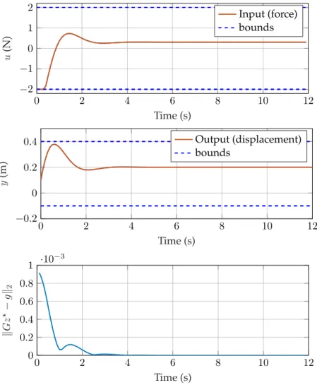
Figure2.1shows a SISO Linear Time-Invariant (LTI) system in which the positionyof a sliding massm= 1.5kg is controlled by an external input forceFagainst the action of a spring with stiffnessκ= 1.5N·m−1_{and a}

damper with damping coefficientc= 0.4N·s·m−1_{. The continuous-time}

model md 2_y dt2 +c dy dt +κy(t) =F(t)

can be converted to the following ARX form (2.2) with a sampling time of 0.1 s and zero-order hold on the input

y(k+ 1) = 1.9638y(k)−0.9737y(k−1) + 0.0033(u(k) +u(k−1)), (2.10) where the input variableu=F.

(36)

m κ

c

F y

Figure 2.1:Mass-spring-damper system.

For MPC we setNp = 10, Nu = 5, Wy = 10,Wu = 1,

√

ρ = 103_.

The maximum magnitude of the input force is2 N, while the mass is constrained to move within 0.4 m to the right and 0.1 m to the left. The output set-pointyr is 0.2 m to the right which implies that the steady-state input referenceuris 0.3 N. The initial condition isy(k) = 0.1 m, y(k−1) = 0andu(k−1) = 0.

Figure2.2shows that offset-free tracking is achieved while satisfying the constraints, and that the controller performance is not compromised by relaxing the dynamic constraints. The bottom plot in Figure2.2shows that the violation of equality constraints is minimal during the transi-ent and zero at steady-state, when there is no inctransi-entive in violating the equality constraints. Finally, Figure2.3analyzes the effect of ρon the resulting error introduced in the model equations.

2.3 Infeasibility handling

Infeasibility may arise while solving (2.8) because output con-straints (2.7b) are not satisfiable at a given sample time, due for instance to unexpected disturbances, modeling errors, or to an excessively short prediction horizonNp. This section investigates the way infeasibility is

handled by the BVLS approach as compared to a more standard soft-constraint approach applied to the MPC formulation based on an I/O model.

(37)

0 2 4 6 8 10 12 −2 −1 0 1 2 Time (s) u (N) Input (force) bounds 0 2 4 6 8 10 12 −0.2 0 0.2 0.4 Time (s) y (m) Output (displacement) bounds 0 2 4 6 8 10 12 0 0.2 0.4 0.6 0.8 1 ·10 −3 Time (s) k Gz ? − g k2

(38)

100 −2 10−1 100 101 102 103 104 105 106 107 108 0.2 0.4 0.6 0.8 1 ·10 −2 ρ max( k Gz ? − g k 2 2)

Figure 2.3: Maximum perturbation introduced in the linear dynamics as a

function of the penaltyρ.

2.3.1 Soft-constrained MPC

We call the “standard approach” when an exact penalty function is used in the formulation to penalize slack variables, which relaxes the output constraints [10, Sect. 13.5], therefore getting the following QP

min u(·),y(·),J(k) +σ1·+σ2· 2 (2.11a) s.t.y(k+l) = na X j=1 Ajy(k−j+l) + nb X j=1 Bju(k−j+l), (2.11b) ¯y(k+l)−¯V ≤y(k+l)≤y¯(k+l) + ¯ V,∀l∈ {1,2, . . . , Np}, (2.11c) ¯ u(k+l)≤u(k+l)≤u¯(k+l),∀l∈ {0,1, . . . , Nu−1}, (2.11d) ≥0, (2.11e)

wheredenotes the scalar slack variable,

¯

V and V¯ are vectors with all elements> 0, andJ(k)as defined in (2.3). The penaltiesσ1 andσ2are

chosen such thatσ1is greater than the infinity norm of the vector of

(39)

0 2 4 6 8 10 12 0 0.1 0.2 0.3 0.4 Time (s) V alue ky(k+ 1)−yˆ(k+ 1)k2

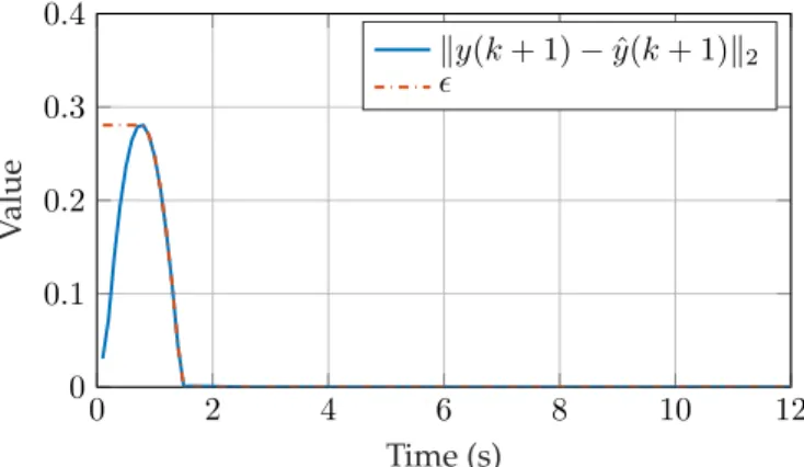
Figure 2.4:Value of slack variableon solving the soft constrained problem

(2.11)and violation of the equality constraint(2.10)at each time step where

ˆ

yis obtained fromzby solving problem(2.9). >0indicates time instants with output constraint relaxation.

order to have a smooth function. This ensures that the output constraints are relaxed only when no feasible solution exists.

2.3.2 Comparison of BVLS and soft-constrained MPC

for-mulations

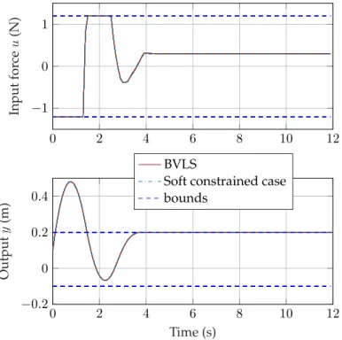
The BVLS approach takes a different philosophy in perturbing the MPC problem formulation to handle infeasibility: instead of allowing a viola-tion of output constraints as in (2.11), the linear model (2.2) is perturbed as little as possible to make them satisfiable.

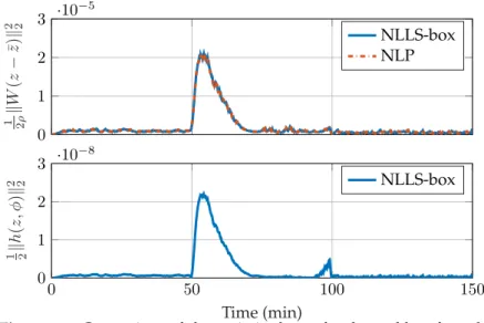
We compare the two formulations (2.9) and (2.11) on the mass-spring-damper system example of Section 2.2.5. In order to test infeasibility handling, harder constraints are imposed such that the problem (2.8) is infeasible, with the same remaining MPC tuning parameters: the max-imum input force magnitude is constrained to be 1.2 N and the spring cannot extend more than 0.2 m. Figures2.4and2.5demonstrate the ana-logy between the two formulations in handling infeasibility. From Fig-ure2.4it is clear that the BVLS approach relaxes the equality constraints

(40)

0 2 4 6 8 10 12 −1 0 1 Input for ce u (N) 0 2 4 6 8 10 12 −0.2 0 0.2 0.4 Time (s) Output y (m) BVLS

Soft constrained case bounds

Figure 2.5: Closed-loop simulation of mass-spring-damper system with

soft-constrained MPC and BVLS formulations.

only when the problem is infeasible, the same way the soft-constraint approach activates a nonzero slack variable. As a result, even though the two problem formulations are different, for this example the traject-ories are almost indistinguishable during times of infeasibility. In order to compare the influence of the relaxations in both cases, we assess the input and output trajectories as shown in Figure2.5. In general, the in-put and outin-put trajectories in the two cases might not be identical as this also depends on how much the equality constraints are relaxed in the BVLS case. In the soft constrained case, the equality constraints are strictly satisfied and only the output inequality constraints are relaxed. In the BVLS case, the box constraints are actually strictly satisfied while solving the problem, however, the outputs violate bounds in reality due

(41)

to the prediction error caused by relaxation of equality constraints.

2.4 Optimality and stability analysis

We analyze the effects of introducing the quadratic penalty function for softening the dynamic constraints (2.4). First, we explore the analogy between the QP and the BVLS problem formulations described earlier. Then, we derive the conditions for closed-loop stability of the BVLS for-mulation. For simplicity, we consider a regulation problem without in-equality constraints, that is we analyze local stability around zero when

¯y(k)<0<y¯(k)andu¯(k)<0<u¯(k). Problem (2.8) becomes min z 1 2kWzzk 2 2 (2.12a) s.t.Gz−g= 0 (2.12b)

(the parentheses indicating the time step have been dropped for simpli-city of notation). Note that the QP (2.12) has a unique minimizer, i.e. (2.12) is strictly convex, ifWz has full rank (implying a positive definite Hessian matrix: Wz>Wz >0) andGhas full row rank (implying linear independence constraint qualification [10]).

By moving the equality constraints (2.12b) in the cost function, we obtain the following unconstrained least-squares problem

min z 1 2 √ ρG Wz z− √ ρg 0 2 2 (2.13) The convergence theory of QPM is well established (cf. [11, Section 17.1]), which clarifies that by using larger values ofρ, one can reduce the sub-optimality caused due to the relaxation of the equality constraints.

Letzρ?be the solution of the least-squares problem (2.13), then it can be expressed as

z?_ρ= (W_z>Wz

| {z }

W

+G>ρG)−1G>ρg, (2.14)

where the matrix(W+G>ρG)is symmetric positive definite, and hence invertible, because it is the sum of a positive-definite matrix (W) with a

(42)

positive-semidefinite matrixG>G. The expression for z?

ρ in (2.14) does not make the influence of ρ on the solution quite apparent. Hence, we next discuss Theorem2.1, which shows that the solutions of (2.12) and (2.13) coincide whenρ→ +∞, a special case of [11, Theorem 17.1], with a detailed alternative proof that provides an intuitive comparison of the analytical solutions of (2.12) and (2.13).

Theorem 2.1 Letz?_and_z?

ρ denote the solutions of problem(2.12)and(2.13)

respectively, withWzassumed to have full rank andGas defined in(2.6). Then asρ→+∞,z? ρ→z?. Proof: G∈RNp·ny | {z } mG ×(Nu·nu+Np·ny) | {z } nG

always has lesser number of rows than columns because clearly,nG > mG. Hence, the equality con-straint (2.12b) can be eliminated using the singular value decomposition (SVD) G=U Σ 0 V₁> V₂> | {z } V> ,

whereU and V are orthogonal matrices and henceV₁>V2 = V2>V1 =

0. As defined in (2.6),Ghas linearly independent rows i.e., Ghas full rank, which implies that it hasmGnon-zero singular values. Hence, the diagonal matrixΣ∈RmG×mG_{, which contains the square root of the} non-zero eigen values ofG>GorGG> in its diagonal entries, is invertible. Solving the system of linear equations (2.12b) gives the following linear system

UΣ 0V>z=g. (2.15)

Letz=V ν=V1ν1+V2ν2. From (2.15) we get

ν1= Σ−1U>g

and problem (2.12) reduces to the unconstrained least-squares problem

min ν2 1 2kWzV2ν2−(−WzV1ν1)k 2 2. (2.16)

(43)

SinceV2∈RnG×(nG−mG)has orthonormal columns,rank(V2) =nG−mG

(full rank). We know that

rank(WzV2)≤min{rank(Wz),rank(V2)}, i.e.,

rank(WzV2)≤nG−mG. (2.17)

From Sylvester’s rank inequality,

rank(Wz) + rank(V2)−nG ≤rank(WzV2), i.e.,

nG−mG ≤rank(WzV2). (2.18)

Comparing (2.17) and (2.18), we infer thatrank(WzV2) =nG−mG, which

implies thatWzV2has full column rank i.e.,(WzV2)>WzV2 >0. Hence,

the solution of (2.16) is unique and may be expressed as ν₂?=−[(WzV2)>WzV2)]−1V2>W > z Wz | {z } W V1ν1 =−(V₂>W V2)−1V2>W V1Σ−1U>g.

Reconstructingzfromν1andν2gives

z?= [I−V2(V2>W V2)−1V2>W]V1Σ−1U>g. (2.19)

Again, using the SVD ofG, problem (2.13) can be rewritten as

min z 1 2 √ ρU Σ 0 V> Wz z− √ ρg 0 2 2 = min z 1 2 _U Σ 0 1 √ ρWzV V>z− g 0 2 2 , (2.20)

sinceV is orthogonal. The solutionz_ρ?of the above least-squares problem (2.20) is computed as follows: V>z?_ρ= _U_Σ ₀ W_√z ρV1 W_√z ρV2 † | {z } Γ† g 0 ,

(44)

whereΓ>Γ>0becauseWzV, and henceΓ, has full column rank, which can easily be proven via the same steps discussed earlier in proving that WzV2 has full column rank. Based on the fact thatV andU are

ortho-gonal, we obtain, z_ρ?=V Γ>Γ−1 Γ> g 0 =V " Σ2₊_V> 1 W ρV1 V > 1 W ρV2 V₂>W_ρ V1 V2> W ρV2 #−1 | {z }   K L M N   −1 ΣU>g 0 .

SinceΓ>Γis a symmetric positive-definite matrix, from the Schur com-plement condition for positive definiteness, we have that the matricesN and(K−LN−1_M₎_{are both positive definite and thus, invertible.}

There-fore, using the matrix inversion lemma, we can write z_ρ?=V ₍_K₋_LN−1_M₎−1 _∗ −N−1M(K−LN−1M)−1 ∗ ΣU>g 0 = V1 V2 ₍_K₋_LN−1_M₎−1_Σ_U>_g −N−1M(K−LN−1M)−1ΣU>g = (V1−V2N−1M)(K−LN−1M)−1ΣU>g =⇒ z_ρ?= (V1−V2(V2>W V2)−1V2>W V1)× Σ2+V > 1 W V1−V1>W V2(V2>W V2)−1V2>W V1 ρ −1 × ΣU>g. (2.21) Evaluating the limit ρ→+∞ on both sides of (2.21) leads to z?

ρ →[I−V2(V2>W V2)−1V2>W]V1Σ−1U>g, i.e.,limρ→+∞z?ρ=z?. Comparingz? _{from (}_2.19_{) with}_z?

ρ in (2.21) shows that a sufficiently large penaltyρmay result in negligible suboptimality. This also explains Figure2.3in which it was observed that the suboptimality introduced

(45)

by penalizing equality constraints monotonically decreases in magnitude with increase in the penalty parameterρ.

Considering that increasing ρinfluences numerical conditioning of problem (2.9), as is the case when using penalty functions in soft-constrained MPC, its value must be tuned to be not too large, depending on the available computing precision. This issue is discussed further in Section3.5.3through a nonlinear system example, which is more challen-ging as compared to the one discussed earlier in Section2.2.5. Next The-orem2.2proves the existence of a lower bound on the penalty parameter ρsuch that, if the MPC controller is stabilizing under dynamic equality constraints, it remains stable under the relaxation via a quadratic penalty function reformulation as in (2.12).

Theorem 2.2 Consider the regulation problem(2.12)and let

ζ(k+ 1) =Aζ(k) +Bu(k)

be a state-space realization of(2.2), which we assume to be stabilizable, such that

ζ(k)_,[(y>(k−n+ 1)· · ·y>(k)) (u>(k−n+ 1)· · ·u>(k−1))]> ∈ Rnζ andn= max(na, nb−1), nζ =n·ny+ (n−1)·nu. The receding horizon

control law can then be described as

u(k) = Λz?(k) = Λ[I−V2(V2>W V2)−1V2>W]V1Σ−1U>S | {z } K ζ(k) (2.22) whereΛ = I 0 · · · 0 ∈ Rnu×(Nu·nu+Np·nζ)_,_g₍_k_{) =} _Sζ₍_k₎_{such that} S = A> 0> ∈ RNp·nζ×nζ_{, and}_K _∈

Rnu×nζ _{is the feedback gain.} Simil-arly, for problem(2.13), referring(2.14), the control law is

uρ(k) = Λz?_ρ(k) = Λ(W +G>ρG)−1G>ρS

| {z }

Kρ

ζ(k) (2.23)

Assuming that the control law(2.22)is asymptotically stabilizing, there exists a finite valueρ∗such that the control law(2.23)is also asymptotically stabilizing

(46)

Proof: Letm _,max(|eig(A+BK)|), whereeig()denotes the set of ei-genvalues of its argument. By the asymptotic closed-loop stability prop-erty of the control law (2.22) we have that

0≤m <1

Letσ= 1_ρ. The continuous dependence of the roots of a polynomial on its coefficients implies that the eigenvalues of a matrix depend continuously on its entries. The continuity property of linear, absolute value, andmax

functions implies thatmax(|eig(A+BK1

σ)|)is also a continuous function ofσand is equal tomforσ= 0. Therefore,

∀γ >0∃δ >0 :

max(|eig(A+BKσ1)|)−m

≤γ,∀0≤σ≤δ (2.24) In particular, for any γ such that 0< γ <1−m we have that

max(|eig(A+BK1

σ)|)<1. Let for exampleγ =

1−m

2 and defineρ

∗ ₌ 1

δ for anyδsatisfying (2.24). Then for anyρ > ρ∗ the corresponding MPC

controller is asymptotically stabilizing.

From Theorem2.2we can thus state the theoretical lower bound on the penalty parameterρto be the solution of the following optimization problem

min ρ

s.t. max(|eig(A+BΛ(W +G>ρG)−1G>ρS)|)<1.

A way to start with an asymptotically stabilizing (non-relaxed) MPC con-troller is to adopt the approach described in [24]. As proved in [24], in-cluding the following terminal constraint

ζ(Np+n−1) = 0χ =ζr (2.25)

guarantees closed-loop stability, where

ζr= [(y>_r · · ·y_r>) | {z } ntimes (u>_r · · ·u>_r) | {z } n−1times

]>∈_Rnζ _{and provided that}_N

p≥n. For the

regulation problem,0χ =0. By substituting (2.2) in the above terminal constraint (2.25), n·ny equality constraints of the form G1z=g1 are

(47)

such equality constraints by penalizing their violation and still guar-antee closed-loop asymptotic stability, provided thatρis a sufficiently large penalty as in Theorem2.2.

2.5 Comparison with state-space model based

approach

We compare our BVLS-based approach (2.9) against the conventional condensed QP approach [10] based on a state-space realization of the ARX model and condensed QP problem

min ξ 1 2ξ >_Hξ₊_f>_ξ _(2.26a) s.t. Πξ≤θ (2.26b)

where ξ ∈ Rnξ _{is the vector of decision variables (i.e.,} predicted inputs and slack variable for soft constraints), nξ=Np·nu+ 1,Π∈R(2Np·(nu+ny)+1×nξ)_, _and _θ_∈

R2Np·(nu+ny)+1 are such that (2.26b) imposes box constraints on the input and output variables, and non-negativity constraint on the slack variable.

We consider the open-loop unstable discrete-time transfer function and state-space model of the AFTI-F16 aircraft [27] under the settings of the demoafti16.min [28]. The system under consideration has 4 states, 2 inputs and 2 outputs. The tuning parameters are the same for both MPC formulations (2.9) and (2.26a) in order to compare the res-ulting performances. As the main purpose here is only to compare the BVLS formulation versus the condensed QP approach based on state-space models (QPss), we use MATLAB’s interior-point method for QP inquadprogto solve the QPss (2.26a), and its box-constrained version to solve2_{BVLS (}_2.9_{). A comparison using state-of-the-art QP solvers for} the same example is included in Chapter4, which discusses the proposed

2_{The MPC problems have been formulated and solved in MATLAB R2015b using sparse}

matrix operations where applicable for both cases in order to compare most efficient im-plementations. The code has been run on a Macbook Pro 2.6 GHz Intel Core i5 with 8GB RAM.

(48)

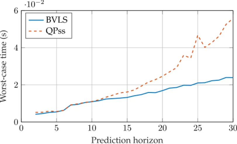
0 5 10 15 20 25 30 0 2 4 6 ·10 −2 Prediction horizon W orst-case time (s) BVLS QPss

Figure 2.6: Simulation results of the AFTI-F16 aircraft control problem:

Worst-case CPU time to solve the BVLS problem based on I/O model and condensed QP (QPss) based on state-space model. The BVLS problem has

4Np variables with8Npconstraints whereas the QP problem has2Np+ 1 variables with8Np+ 1constraints.

BVLS solver in detail. It is worth noting that for the considered example, due to unstable open-loop dynamics, the Hessian matrix in (2.26a) tends to become ill-conditioned with increase in the prediction horizon and beyond a certain large value it can even cause numerical overflow. This is clearly because the Hessian contains higher powers of the system mat-rix, therefore scaling its eigen values with the prediction horizon.

Figure 2.6 shows that even though the BVLS problem has almost twice the number of primal variables to be optimized, it is solved faster due to simpler constraints. However, this benefit due to simpler con-straints strongly depends on the solution algorithm. This also motivates the research on solution algorithms that best exploit the simplicity of the optimization problem, which is discussed in Chapter4.

Fewer computations are involved in constructing the BVLS problem (these are online computations in case of linear models that change in real time) as compared to the condensed QP one, as shown in Figure 2.7. This makes the BVLS approach a better option in the LPV setting,

(49)

0 5 10 15 20 25 30 0.5 1 Prediction horizon T ime (ms) BVLS QPss

Comparison of the CPU time required to construct the MPC problems(2.9) and(2.26a)against prediction horizon.

0 5 10 15 20 25 30 0 0.1 0.2 0.3 0.4 0.5 Prediction horizon W orst-case time (ms) BVLS QPss

Comparison of the worst-case CPU time required to update the MPC prob-lem before passing to the solver at each step.

(50)

where the problem is constructed on line. Moreover, even in the LTI case one has to update vectorsθ,g on line. Figure2.8shows that the BVLS approach requires fewer computations for such a type of update. Note also that the computations required for state estimation (including constructing the observer matrices in the LPV case) that is needed by the condensed QP approach have not been taken into account, which would make the BVLS approach even more favorable.

2.6 Conclusions

In this chapter we have proposed an MPC approach based on linear I/O models and BVLS optimization. The obtained results suggest that the BVLS approach may be favorable in both the LTI and adaptive (or LPV) case, and especially for the latter case it may considerably reduce the on-line computations. A potential drawback of the BVLS approach is the risk of numerical ill-conditioning due to the use of large penalty val-ues, an issue that could appear also in soft-constrained MPC formula-tions. This issue is addressed in Chapter4 which describes a numeric-ally robust BVLS solver that is well-suited for the considered problems. Furthermore, an implementation that exploits structure of the proposed MPC problem formulation and is efficient in terms of both memory and computations is discussed in Chapter6.

(51)

Chapter 3

Nonlinear model predictive

control problem

formulations

3.1 Introduction

Nonlinear Model Predictive Control (NMPC) is a popular control strategy which is able to deal with constrained nonlinear systems. How-ever, a common obstacle is the need for solving a nonconvex optimiza-tion problem within a stipulated sampling period. A common approach in tackling this issue is developing efficient algorithms tailored to NMPC problems. Often, a suboptimal solution which can be computed fast and efficiently is preferred over a precise one that requires longer computa-tional times [5]. Many different tools have been developed for this pur-pose, see e.g. [29–35]. In this work instead, we follow a different ap-proach and formulate the NMPC problem in a simple way such that it becomes possible to employ existing fast optimization algorithms.

The quadratic penalty method (QPM) [11] converts a constrained nonlinear optimization problem to a sequence of unconstrained ones, which are solved suboptimally such that the penalty parameter is in-creased at each instance, until a solution that satisfies termination criteria

(52)

is achieved. Using a large enough value of the penalty parameter yields an approximately optimal solution in a single iteration. The need of ad-equately selecting the penalty parameter to balance accuracy of the solu-tion and ill-condisolu-tioning of the problem made this approach not the most appealing for general-purpose solvers. In NMPC, however, small con-straints violations are typically negligible compared to model inaccuracy and external perturbations acting on the system. Therefore, the quad-ratic penalty method is very appealing for such applications due to the possibility of developing efficient implementations. Similar to the linear MPC case, we propose to use a single iteration of the quadratic penalty method which keeps simple bounds on the decision variables as such and relaxes the equality constraints via a quadratic penalty function. The obtained problem is bound-constrained nonlinear least-squares (NLLS), which can be solved by employing the Gauss-Newton method [21] and a Bounded-Variable Least-Squares (BVLS) solver, which is both efficient and numerically robust.

As opposed to standard infeasibility handling approaches which re-lax the output constraints [19,30], we relax the equality constraints re-lated to the model of the system. As discussed earlier, the main motiv-ations for such a choice are that 1) it preserves feasibility of the optim-ization problem, similarly to the output constraint relaxation, and 2) the available model is an approximate representation of the true system.The benefits of the proposed method are demonstrated and summarized with an example that is commonly considered in the NMPC literature. In par-ticular, we show that the constraint violation is not significant unless the original problem becomes infeasible, and therefore, the control perform-ance is not deteriorated.

We first define in Section 3.2 the class of models, perfomance in-dex, and constraints that are typically considered for formulating NMPC problems. Based on that, the benchmark NMPC problem formula-tions which we consider are described in Section3.3, whereas the pro-posed NMPC formulation based on an iteration of the quadratic penalty method is described in Section 3.4, including a brief discussion on an alternative approach based on the augmented Lagrangian method [11].

(53)

Numerical results and their discussion are presented in Section3.5with concluding remarks in Section3.6.

Notation. For a vectora∈Rm, itsp-norm iskakp,jth element isa(j). The set of integers in the closed interval betweenaandb is denoted as

[a, b]. The remaining notation is same as described in Chapter2.

3.2 Preliminaries

We describe the system dynamics by using the following discrete-time input-output model

f(Yk, Uk, Vk) =0, (3.1)

where we define the inputs and outputs, respectively, at a given discrete-time step k as Uk= (uk−nb, . . . , uk−1), uk∈R nu_, _Y k= (yk−na, . . . , yk), yk∈Rny_. _Vector _V k= (vk−nc, . . . , vk−1), vk∈R nv _{defines a}

meas-ured disturbance and 0 represents a zero vector. Function

f :_Rnany ×

Rnbnu×

Rncnv →

Rny _{is in general nonlinear, where} _n

a, nb

andnc define the model order. We assumef to be differentiable. The

class of nonlinear models of the form (3.1) includes, for instance, state-space models and the noise-free polynomial NARX (nonlinear autore-gressive exogenous) models [36].

As discussed in the case of linear MPC, we consider a convex quad-ratic performance index ‘P’, which is separable in time and a typical choice for regulation and reference tracking in MPC:

P(k) = Np X j=1 1 2kW 1 2 y(yk+j−y¯k+j)k22+ Nu−2 X j=0 1 2kW 1 2 u(uk+j−u¯k+j)k22 +1 2(Np−Nu+ 1)· kW 1 2 u(uk+Nu−1−u¯k+Nu−1)k 2 2, (3.2)

where Np and Nu denote the prediction and control horizon

respect-ively. MatricesWy∈Rny×ny _and_W

u∈Rnu×nu _{are positive} semidefin-ite tuning weights, andy¯, u¯ denote the references for outputs and in-puts, respectively. In general, the proposed NMPC approach described in Section3.4is not limited to the above-mentioned performance index. Depending on the control objectives, any cost function that results in a

(54)

sum of squares of linear or differentiable nonlinear functions may be con-sidered in order to formulate the NMPC problem.

In order to exploit an efficient solution algorithm, the only inequality constraints that we consider are simple bounds on the optimization vari-ables. Generalsoftinequality constraints (3.3) can be converted to the considered setting by introducing slack variablesν ∈ Rni _having

non-negativity constraints such that

g(wk)≤0 becomes, (3.3)

g(wk) +νk =0 and νk≥0,

where wk = (uk, . . . , uk+Nu−1, yk+1, . . . , yk+Np), zk= (wk, νk);

g:R(nz−ni)_→

Rni _{is assumed to be differentiable, while} _nz _and _n

i

denote the number of decision variables and general inequality con-straints, respectively. We summarise all NMPC constraints at each time stepkas

h(zk, φk) =0 (3.4)

pk ≤zk ≤qk (3.5)

wherepk, qk are vectors defining bounds on the input and output vari-ables, and non-negativity constraint on the slack variables. Vector φk = (uk−nb+1, . . . , uk−1, yk, . . . , yk−na+1) denotes the initial condition.

Some components of zk may be unbounded and in that case those bounds are passed to the proposed solver as the largest negative or posit-ive floating-point number in the computing platform. Hence, practically, pk, qk ∈ Rnz_{. Owing to the construction of equalities (}_3.4_{), it is worth} noting that the Jacobian matrix ofhw.r.t.zevaluated at any givenzk is sparse, with its sparsity pattern depending on the chosen model (3.1).

3.3 Conventional formulations

3.3.1 Constrained NLP

Employing the performance index (3.2) and the constraint set defined by (3.4) and (3.5), the NMPC problem can be defined as the following

Bounded-variable least-squares methods for linear and nonlinear model predictive control

IMT School for Advanced Studies Lucca

Lucca, Italy