Optimal Load-Balancing
Isaac Keslassy
1Cheng-Shang Chang
2Nick McKeown
3Duan-Shin Lee
21
Technion
2National Tsing Hua University
3Stanford University
Haifa, Israel
Hsinchu, Taiwan, R.O.C.
Stanford, CA, U.S.A.
[email protected]
{
cschang@ee,lds@cs
}
.nthu.edu.tw
[email protected]
Abstract— This paper is about load-balancing packets across multiple paths inside a switch, or across a network. It is motivated by the recent interest in load-balanced switches. Load-balanced switches provide an appealing alternative to crossbars with centralized schedulers. A load-balanced switch has no scheduler, is particularly amenable to optics, and – most relevant here – guarantees 100% throughput. A uniform mesh is used to load-balance packets uniformly across all 2-hop paths in the switch. In this paper we explore whether this particular method of load-balancing is optimal in the sense that it achieves the highest throughput for a given capacity of interconnect. The method we use allows the load-balanced switch to be compared with ring, torus and hypercube interconnects, too. We prove that for a given interconnect capacity, the load-balancing mesh has the maximum throughput. Perhaps surprisingly, we find that the best mesh is slightly non-uniform, or biased, and has a throughput of N/(2N−1), whereN is the number of nodes.
I. INTRODUCTION A. From Scheduling to Load-Balanced Routing
Current Internet core routers commonly implement com-bined input and output queueing (CIOQ) with a centralized scheduler. Numerous centralized scheduling algorithms have been proposed in the literature [1], [2], [3], [4]. Nevertheless, although these scheduling algorithms can theoretically provide a guaranteed throughput of 50% to100%([5], [6], [7]), they are becoming impractical as the line rates and number of ports grow, because of their complexity and/or the speedup of the buffer memory.
There has been recent interest in a new approach, which eliminates scheduling, using a load-balanced switch architec-ture [8], [9], [10], [11], [12], [13], [14]. As shown in [12], this architecture appears to be a practical way to scale In-ternet routers to very high capacities, and achieve throughput guarantees for all traffic patterns.
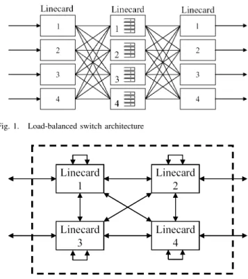
Figure 1 shows the load-balanced switch architecture based on two fully-interconnected meshes, with N = 4 linecards interconnected by N2 links. It consists of a single stage of
buffers sandwiched by two identical stages of switching, where each switch is built from a uniform mesh. Each linecard in the This research was supported by the Wakerly Stanford Graduate Fellowship, by the ATS-WD Career Development Chair, by the National Science Council, Taiwan, R.O.C., under contract NSC-91-2219-E007-003, by the Program for Promoting Academic Excellence of Universities, under contract NSC-94-2752-E-007-0PAE, by the NSF Large ITR grant under contract NSF 02-168, by the DARPA/MARCO Center for Circuits, Systems and Software under MARCO contract 2001-CT-888 and DARPA grant MDA972-02-1-0004, and by Cisco Systems.
Fig. 1. Load-balanced switch architecture
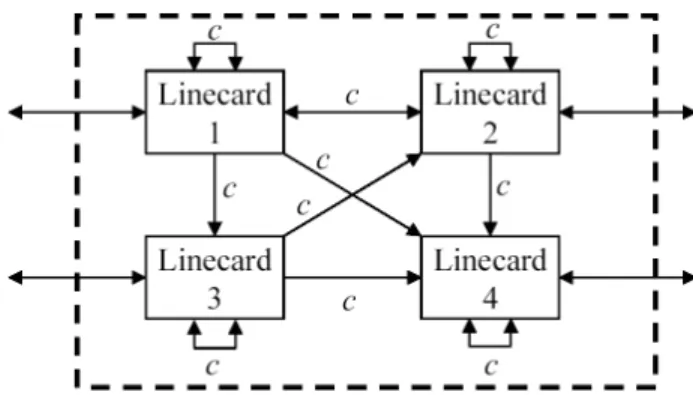
Fig. 2. Generic architecture of a load-balanced switch and of a load-balanced routing network
first stage is connected to each linecard in the center stage by a channel at rate R/N, where R is the line rate and N is the number of linecards. Likewise, each linecard in the center stage is connected to each linecard in the final stage by a channel at rate R/N. The buffer at each center stage is par-titioned into N virtual output queues (VOQs). To understand its operation, consider a stream of packets from a given input to a given output. The first mesh sends packets in round-robin to all intermediate inputs, load-balancing traffic across them. Each packet is put into the VOQ in the intermediate input according to its eventual output. The second mesh services each VOQ at fixed rate R/N, regardless of its occupancy. Each packet is transferred across the second mesh to its output, from where it departs the system. Thus, the two meshes work identically, but perform two different functions: the first one load-balances packets across the center stages, sending 1/N -th of -the traffic to each intermediate input, and -the second one switches packets to their correct destination by servicing each VOQ at fixed rate R/N.
each stage), a real implementation would have N linecards, and each linecard would contain three logical parts (input, intermediate input and output). This means that the two meshes can be replaced by a single mesh running twice as fast, as shown in Figure 2. Every packet traverses the switch fabric twice: once from the input linecard to a VOQ in the intermediate linecard, then a second time from the VOQ to the output linecard.
B. The Throughput of Load-Balanced Switching
Perhaps the most interesting characteristic of the load-balanced switch is that it provably achieves 50% throughput (and therefore 100% throughput with a speedup of two) for a broad class of weakly mixing, stochastic arrivals [8]. Intuitively, the first stage makes traffic (just) uniform enough for the second stage to provide the throughput guarantee.
It is not immediately obvious why a load-balancing stage built from a uniform mesh withNinputs and outputs can make the traffic uniform enough, regardless of the traffic matrix or the burstiness of the arrivals. And it’s even less obvious whether the mesh needs to be uniform (i.e. all links have the same capacity R/N); how does the throughput change if the mesh is non-uniform? What arrangement of link capacities maximizes the throughput?
More generally, we’re interested in comparing the architec-ture with other well known ways to interconnect linecards. For example, a ring, a torus or a hypercube. We’ll compare them by considering an interconnection network with a given total capacity. Packets are routed through the network to create a load-balanced switch, a ring, torus, or hypercube. We then determine which arrangement has the highest throughput.
To make the comparison, we’ll use an arbitrary network with fixed capacities that we’ll call a load-balanced routing network. As in the load-balanced switch, linecards are inter-connected using a network with a fixed configuration and fixed capacities (Figure 2). Each incoming flow can be load-balanced across the different possible paths to its output, as long as the rate needed on each link is within its capacity. For each flow, a decision has to be made: how should it be load-balanced across the different possible paths?
Consider the example in Figure 3. It shows a simple load-balanced routing network where all the capacities between linecards are either zero (no link) or c. If linecard 1 wants to send traffic to linecard 4, it could send it directly using the link 1 → 4 (with capacity c). It could also choose to load-balance traffic using the paths 1 → 2 → 4, 1 →3 →4, or
1 →3 →2 →4. We’ll allow it to choose any path, even if it’s obviously not useful, such as 1 → 3 → 2 → 1 → 4 or
1→1→1→4→4.
Essentially, what is normally a schedulingdecision inside the router is transformed into a routing decision. While a centralized scheduler needs to decide how to configure a crossbar depending on the queue state, the linecards in a load-balanced routing network need to decide how to route flows across the different possible internal paths.
The general class of load-balanced routing networks ap-pears in many areas of networking. Perhaps most commonly,
Fig. 3. Example of load-balanced routing network
load-balanced routing networks are an example of multi-path routing [15], [16], [17] in a network, or Internet, of routers. They are also commonly used in torus and hyper-cube networks [18], [19] for the implementation of multi-stage, distributed switches inside routers [20], multiprocessor interconnection networks [21] and I/O interconnects [22]. For each flow, the path taken by the packets might then be pre-determined without regard to the state of the system (also called oblivious routing [23], which includes Valiant’s random-ized routing [24]); or adaptive (where routing is dependent on the queue state [25]). Load-balanced routing networks can also be used in fixed ad-hoc networks, such as sensor networks [26], [27]. Finally, load-balanced routing networks are a specific type of multi-commodity network that often appears in the networking literature. Understanding their the-oretical bounds would be useful to the general class of multi-commodity network problems.
C. Main Results
We will analyze the throughput of load-balanced routing networks. The main findings of this paper are as follows. First, the throughput as a function of the capacity of load-balanced routing networks is concave, strictly increasing, and scales linearly. Second, a switch based on a uniform mesh has a guaranteed throughput of 50%, and so needs a speedup of two (or two meshes) to achieve 100% throughput. The uniform mesh is close, but not equal to, the interconnection with the highest throughput. A slightly biased, non-uniform mesh has a slightly higher throughput. In particular, the following is true: Theorem 1: The capacity matrix with the best throughput exists and is unique. It is
ˆ C= 1 2N−1 · 1 2 . . . . . . 2 2 1 . .. ... .. . . .. ... ... ... .. . . .. 1 2 2 . . . . . . 2 1 ,
and its throughput isN/(2N−1)>1/2.
The reason is quite simple: In a uniform mesh, each node spreads traffic - and so routes packets - equally to all other nodes. But spreading to itself is redundant and inefficient. For instance, if node 1 has traffic to send to node 2 and the direct
link1→2is congested, it can use load-balancing by sending part of this traffic to node 3, which will forward it to node 2. However, it is useless to send part of this traffic to node 1 for load-balancing, since this action just makes some packets come back to their starting point. Therefore, a link from a node to itself needs less capacity than a link from a node to another one, resulting in a non-uniform mesh. But asymptotically, for large N, the throughputs of the uniform and optimal meshes are the same.
In what follows we start by formulating more precisely the optimization problem in Section II, illustrate the definition of the guaranteed throughput in Section III, and provide its main properties in Section IV. Then, we describe the biased full mesh and compute its guaranteed throughput in Section V, show that its guaranteed throughput is optimal in Section VI, and prove that it is the only architecture with such a guaranteed throughput in Section VII. Finally, we analyze the load-balancing gain of an arbitrary architecture in Section VIII. All the proofs are in the Appendix.
II. PROBLEMFORMULATION A. Notations and Assumptions
Consider a network with N identical nodes, whereN ≥2. We define a doubly stochastic matrix to be a non-negative square matrix with all row and column sums equal to 1. Similarly, we define anadmissible (or doubly sub-stochastic) matrix to be a non-negative square matrix with all row and column sums upper-bounded by1. Finally, we define the time unit such that each node can send and receive at most one bit per second (if the maximum node speed is R, scale the time unit by a factor R1).
A link of fixed capacity Cij connects node i to node j,
where 1 ≤ i, j ≤ N. The matrix C = [Cij]1≤i,j≤N is the
capacity matrix, and any node l can send up to Nj=1Clj
(and likewise receive at mostNi=1Cil) bits per time unit to
and from the N nodes (including itself). Since every nodelcan send and receive at most one bit per time unit, Ni=1Cil≤1
and Nj=1Clj ≤ 1; therefore, the matrix C is admissible.
The capacity matrix C defines the architecture; for example, the uniform mesh architecture(in which nodes are connected to each other with equal-capacity links), corresponds to the uniform matrix C where Cij = 1/N.Similarly, a ring could
be defined byCij =1{j=i+1 modN}.
Denote by T the arrival traffic rate matrix, with Tij being
the arrival rate at node i of packets destined for node j. We will assume thatT is admissible, since it cannot be supported otherwise: each node can send and receive at most one bit per second. Suppose we want to load-balance these packets across multiple paths, each path having an arbitrary number of hops. If P(i, j) is the set of paths between nodes i and j, then any path p ∈ P(i, j) can be represented as (i → node1 →
node2→. . .→j). LetTijp be the rate of the flow carried byp. If the arrival traffic rate matrixT is feasible (i.e., the network has 100% throughput for T), it is possible to decompose T
into several paths p, and therefore for alli, j,
Tij =
p∈P(i,j)
Tijp. (1)
Similarly, we will define the effective load matrixLusing for alli, j:
Lij=
{p:(i→j)∈p}
Tijp. (2)
The effective load of a link is the sum of the loads of the paths sharing the link. A solution is feasible if and only if we can find a decomposition of T such that L ≤ C, i.e., no link is over-booked.
B. Problem Intuition
Suppose that N = 2 and that we use a uniform mesh architecture, with capacity matrix
C= 0.5 0.5 0.5 0.5
.
We will use this example to gain some intuition about the throughput of interconnection networks.
If the arrival rate matrix is
T1= 0.9 0
0 0
then we cannot send traffic at rate 0.9 on the path 1 → 1, because the capacity is limited byC11 = 0.5. Therefore, we
need to load-balance the traffic by using the spare capacity of other links. We will send0.5 on the direct path 1 →1, and the remaining 0.4 on the alternative path 1 → 2 → 1. The resulting load matrix is
L1= 0.5 0.4 0.4 0
,
andL1 ≤C.Clearly, the direct path is not always sufficient
to carry the required rate matrix, but in this case it is possible to use a load-balanced path in order to carry it.
Not all rate matrices are feasible, i.e., the throughput is not always100%. Consider the arrival rate matrix
T2= 0.9 0
0 0.9
.
Sending0.5on1→1,0.4 on1→2→1,0.5 on2→2 and
0.4on2→1→2, the load matrix is
L2= 0
.5 0.8 0.8 0.5
,
and soL2≤C. In this particular case, we need to scale down
T2 to
0.75 0 0 0.75
for the solution to be feasible.
Finally, load-balancing does not always help, particularly in small matrices when there are not many paths to divert traffic away from congested links. And it is always useless to divert traffic to oneself. For example, consider the rate matrix
T3= 0 0.5 +
0.5 0
,
where > 0. Sending traffic on the path 1 → 1 → 2 does not divert traffic from the congested link 1 → 2; therefore,
T3 is not feasible. This teaches us that when sending traffic from nodeito nodej =i, it is clearly useless to use the link
i → i, because traffic is transferred across the network with no benefit. By comparing T1, T2 and T3, this example also
shows that finding the maximum throughput of a given rate matrix is not straightforward, even when N = 2. Moreover, since the number of cases to consider increases withN, such a problem is increasingly difficult to solve as N grows. C. Problem Definition
Our objective is to find the load-balanced network with the largest throughput guarantee. In other words, we want to find a network with a guaranteed throughputθ∗, whereθ∗ satisfies two properties. First, given any admissible arrival traffic, the network guarantees a throughput θ∗, i.e., it will switch a fractionθ∗of the traffic for any input-output flow. And second, no other network can have a better guaranteed throughput than θ∗. We will define the problem by decomposing it into three successive optimization problems. First, we will find the throughput for a given network and a given rate matrix. Then, we will obtain the worst-case throughput of a network, which can be achieved for any rate matrix. Finally, we will provideθ∗, which is the best guaranteed throughput among all networks.
In the first optimization, we want to find the maximum throughput for a given network and a given rate matrix. In other words, given capacity matrix C and rate matrixT, we want to find the best possible throughput θ(C, T), such that the scaled-down rate demand matrixθ(C, T)×T is feasible. Put mathematically, θ(C, T)≡max θ (θ), subject to: (i) Pp=1(i,j)T p ij =θ×Tij ∀i, j (ii) L(i, j)≡{p:(i→j)∈p}T p ij ≤Cij ∀i, j (iii) Tijp ≥0 ∀i, j, p
In words, the throughputθ(C, T)is the maximum of the set of throughputs θthat satisfy three feasibility conditions. First, the arriving traffic is a scaled-down version of T by a factor
θ, such that it can be decomposed into several pathsp. The second condition is that the sum of the loads of the paths must be less than C, i.e., that the load matrix is feasible. The last condition is that the rate on each path must be nonnegative.
The second optimization finds the guaranteed maximum throughputθ(C) for the network. This is the throughput that is achievable by any rate matrix in the network, and, therefore,
θ(C)≡ min
T admissible(
θ(C, T)). (3)
Note that we allow for any admissible rate matrixT, because the network should be able to support any traffic shape, as long as the traffic originating from (and destined to) each node does not exceed one bit per second.
Finally, we find the maximum possible guaranteed through-put for any network, yielding a guaranteed throughthrough-put θ∗, where
θ∗≡ max
C admissible(
θ(C)). (4)
III. EXAMPLES OFGUARANTEEDTHROUGHPUT A. Guaranteed Throughput of the Uniform Mesh
The uniform mesh is an architecture in which all links have the same capacity, i.e.,Cij = 1/N for all i, j. We will show
that the maximum guaranteed throughput of the uniform mesh is50%.
We saw already in the Introduction why the uniform mesh guarantees at least 50% throughput, although the proof was based on slightly different assumptions. This guarantee was first shown by Valiant [28]. In short, each packet goes through both the load-balancing stage and the forwarding stage, and therefore through two hops. Consequently, the link between nodeiand nodejcan receive load in two possible ways. Either nodei is sending traffic to some nodek and spreads it using the intermediate nodej, or some nodelsends traffic to nodej
and spreads it using the intermediate nodei. Mathematically,
Lij =
kTik+
lTlj≤2with an admissibleT. Therefore,
θ(C)≥50%.
The following example shows that it is not possible to do better using a different load-balanced routing algorithm. Assume that T = 0 x 0 . . . 0 0 0 x . .. ... .. . . .. ... 0 0 0 x x 0 . . . 0 0 ,
where x≥1/2. A node ican send at most Ci(i+1 modN)=
1/N amount of traffic directly.1 It also needs to send the remainingx−1/N amount of traffic to load-balanced paths, with each of these paths using at least two links. Hence, the total traffic load contributed by each node to the system is at least (1/N) + 2(x−1/N), which implies that the total traffic load contributed by the N nodes is N(1/N+ 2(x− 1/N)) = 2N x−1. As we saw earlier, diagonal elements do not help load-balancing, and with this rate matrix they are also useless for direct paths. Hence, the total useful traffic capacity is the sum of all non-diagonal elements of C, i.e.,
N·(1−1/N) = N−1. For the solution to be feasible, we need 2N x−1≤N −1, which translates intox≤1/2. And so there exists a traffic rate matrix that is only feasible with a throughput of at most50%. This impliesθ(C)≤50%. Since we found that the two-hop algorithm provides a throughput of
50%, it follows that
θ(C) = 50%. (5) Further, it is not possible to improve on the two-hop algorithm. B. Guaranteed Throughput of a Ring
As a second example, consider a network in which the nodes are connected in a uni-directional ring, i.e., nodeiis connected to node (i+ 1) modN. Recall that we assumed that each packet needs to go at least once through the network. In the
1The modulo function takes values in{1, ..., N}when nodes are numbered {1, ..., N}.
worst case, T is the identity matrix so that nodes only send traffic to themselves through the ring. Therefore, all packets crossNlinks, and the throughputθ(Cring, T)is equal to1/N.
ThisTis the worst case, since packets do not need to use more thanN links to reach their destination. Therefore,
θ(Cring) = 1/N, (6)
which — as expected — is much lower than for the uniform mesh.
C. Guaranteed Throughput of a Permutation Matrix
The ring is a special case of a permutation matrixσof the set {1, ..., N}, where σ is the capacity matrix of a network. The matrixσcan be represented as a0−1matrix with exactly one 1 in each row and column; i.e., σij = 1 if σ(i) = j,
and σij = 0 otherwise. Since σ is a permutation, it can be
decomposed as a product of disjoint cycles (the decomposition is unique up to the order of the cycles).
If σ can be written as a single cycle of lengthN, we can assume without loss of generality thatσ(1) = 2,σ(2) = 3,...,
σ(N) = 1, and so σ is the capacity matrix of a ring, with
θ(σ) = 1/N.
Alternatively, if σcan be written as the product of two or more cycles, then there are two nodesiandjsuch that nodei
is in the first cycle and node jis in the second one. It is then impossible to reach nodej from nodei(the capacity graph is not connected), hence the throughput for any matrix T such that Tij= 1 is zero, and θ(σ) = 0.
This example illustrates that the throughput of a capacity matrix is sensitive to its coefficients; and that the throughput of a disconnected graph is zero.
IV. PROPERTIES OF THEGUARANTEEDTHROUGHPUT In the above examples, we computed the throughputs of several capacity matrices, but found that it is not straight-forward in general to compute throughput directly. Since we want to find the capacity matrix with the largest guaranteed throughput, we will use general properties of the throughput function. We will start by showing that it is concave in C, scales linearly, and is strictly increasing.
A. Concavity
First, we show that throughput is concave in C. Assume that two capacity matricesC1 andC2 achieve throughputs of
θ(C1, T) and θ(C2, T) for a rate matrix T. Then, applying the definition of throughput, for any λ ∈ [0,1], the matrix
C=λC1+ (1−λ)C2 will achieve a throughput ofθ(C, T)≥
λθ(C1, T) + (1−λ)θ(C2, T). This can be seen by using the
paths from C1 for a fraction λ of the traffic, and the paths
fromC2for a fraction1−λ. As a consequence, we also have
θ(C)≥λθ(C1) + (1−λ)θ(C2). This leads to the following
proposition.
Proposition 2: The guaranteed throughput functionθ(C)is concave in C.
B. Linear Scaling
Given any positiveλ, we can find a feasible rate allocation forλCfrom the rate allocation forC(and vice versa) by scal-ing the rate assigned to each path by a factorλ(respectively by 1λ). Therefore, we get the following proposition:
Proposition 3: The guaranteed throughput function θ is linear with respect to scaling, i.e.,
θ(λ·C) =λ·θ(C).
C. Strictly Increasing
Clearly θ is a non-decreasing function in the space of admissible capacity matrices. In other words, having more capacity cannot decrease the throughput. IfC andD are two admissible capacity matrices, where C≤D (i.e., for all i, j,
Cij ≤ Dij, defining a partial order relation), then from the
definition ofθ:θ(C)≤θ(D).
Now, ifD > C, there exists such that
D≥C+Cuniform,
where Cuniform is the capacity matrix of the uniform mesh. Hence θ(D) (≥a) θ((1 +)( 1 1 +C+ 1 +Cuniform)) (b) = (1 +)×θ( 1 1 +C+ 1 +Cuniform)) (c) ≥ (1 +)( 1 1 +θ(C) + 1 +θ(Cuniform)) (d) = (1 +)( 1 1 +θ(C) + 1 + 1 2)) > θ(C),
where (a) uses the fact that θ is non-decreasing, (b) uses the equalityθ(λ·C) =λθ(C), (c) uses the concavity ofθand (d) uses the value ofθ(Cuniform). Therefore, we obtain:
Proposition 4: The guaranteed throughput function θ is strictly increasing, i.e., if C < Dthenθ(C)< θ(D).
V. THEBIASEDMESH A. Definition
We have already seen that the uniform mesh has a through-put of50%, even though a node potentially spreads traffic over the useless links to itself. We can therefore expect a modified mesh — i.e., a mesh that does not spread traffic to itself — to have higher throughput. This is indeed the case; in fact, it is the network with the highest guaranteed throughput.
In this modified mesh, a link from a node to itself is only used to send traffic directly, and not for spreading. However, a link from a node to another one is used for sending traffic directly as well as for spreading. Therefore, intuitively, a link from a node to another one should have twice as much capacity as a link from a node to itself, because it will be used for two functions instead of one. We will call such a modified mesh thebiased mesh. Its capacity matrix Cˆ is given by
ˆ C= c 2c . . . . . . 2c 2c c . .. ... .. . . .. ... ... ... .. . . .. c 2c 2c . . . . . . 2c c , where c= 1/(2N−1).
In the remainder (Propositions 6, 7 and 8), we will show that Cˆ uniquely achieves the highest guaranteed throughput, using three consecutive steps. First, we will show that Cˆ
achieves a throughput of N/(2N−1). Then, we will prove that this is the largest achievable throughput for any network. Finally, we will demonstrate that the biased mesh is the only network to achieve this throughput.
B. Guaranteed Throughput of the Biased Mesh
Our first objective is to show that the guaranteed throughput of the biased mesh with the capacity matrix Cˆ is at least
N/(2N−1). Using the definition of the guaranteed throughput, we need to consider all admissible rate matrices T. The following proposition significantly restricts the number of rate matricesT we need to consider. It is proved in Appendix I.
Proposition 5: The guaranteed throughput θ(C) defined in (3) can be found by considering the set of permutation matrices, i.e.,
θ(C) = min
T permutation(
θ(C, T)). (7)
Proposition 5 restricts to the set of permutation matrices the set of rate matrices we need to consider. To show that the throughput of Cˆ is at leastN/(2N −1), we just need to show that a throughput ofN/(2N−1)can be achieved for all the permutation matrices. It leads to the following proposition, proved in Appendix I.
Proposition 6: The guaranteed throughput of the biased mesh with capacity matrixCˆ is at leastN/(2N−1).
VI. OPTIMALITY OF THEBIASEDMESH
We have just found that the biased mesh guarantees a throughput of at least N
2N−1. The following proposition shows
that the biased mesh achieves the maximum possible guaran-teed throughput for any admissible capacity matrix.
Proposition 7: If the capacity matrixC is admissible, then its guaranteed throughput satisfies
θ(C)≤ N 2N−1.
The proof for Proposition 7 is in Appendix II.
VII. UNIQUENESS OF THEOPTIMALCAPACITYMATRIX Since we proved that the biased mesh achieves the optimal throughputN/(2N−1), we will now demonstrate that it is the only capacity matrix to do so. This is done in Proposition 8, proved in Appendix III.
Proposition 8: The only capacity matrixCthat can achieve the optimal throughputN/(2N−1)is the capacity matrixCˆ
of the biased mesh.
In conjunction with Propositions 6, 7 and 8, we have, therefore, established the following theorem.
Theorem 9: The biased mesh satisfies the following three properties:
(i) The guaranteed throughput of the biased mesh is equal toθˆ=N/(2N−1).
(ii) The biased mesh achieves the maximum possible guaran-teed throughput for any network, i.e.,θ( ˆC) =N/(2N− 1).
(iii) The biased mesh is the only network to achieve this guar-anteed throughput, i.e.,θ(C)< θ( ˆC)for any admissible capacity matrixC= ˆC.
VIII. THEBENEFIT OFLOAD-BALANCING
We can now quantitatively analyze the benefits of load-balancing in anarbitrarynetwork. Put mathematically, we can estimate the ratio of the guaranteed throughputs that can be achieved when load-balancing is allowed and when it is not. We will call this ratio theload-balancing gain.
A. Guaranteed Throughput without Load-Balancing
Let’s compute the guaranteed throughput without load-balancing, when only direct links can be used. To go from nodei to nodej, a packet must be sent over the unique link betweeniandj, and cannot be load-balanced via a third node. In general, the guaranteed throughput of a non-load-balanced network will be determined by its weakest link, as can be seen when using a rate matrix that fully uses the weakest link. Thus, the guaranteed throughput of a capacity matrixC will be
min
i,j Cij.
For instance, without load-balancing, the guaranteed through-put of the uniform full mesh is 1/N, and the guaranteed throughput of the biased full mesh is1/(2N−1).
B. Guaranteed Throughput with Load-Balancing
Let’s now bound the guaranteed throughput with load-balancing so as to bound the benefit of load-load-balancing. From Theorem 9, we know that the guaranteed throughput of a network is upper-bounded by θˆ, but we need to find a lower-bound on the guaranteed throughput. We can do it by comparing the network to the biased full mesh, which has the highest guaranteed throughput. Using the linear scaling and monotonicity properties of the throughput function, we find that for anyλ∈[0,1],
C≥λCˆ⇒θ(C)≥λθ.ˆ
In other words, if a given network has at least as much capacity as the scaled-down version of the biased full mesh, then it will also provide at least as much guaranteed throughput as the scaled-down guaranteed throughput of the biased full mesh. We can obtain the following proposition:
Proposition 10: The guaranteed throughput θ(C) for any capacity matrixC satisfies:
ˆ θ·min i,j C ij ˆ Cij ≤θ(C)≤θ.ˆ
C. Load-Balancing Gain
Define the load-balancing gain as the ratio of the guaranteed throughputs with and without load-balancing. Mathematically,
l.b.gain= θ(C) mini,jCij
.
The load-balancing gain is a measure of the gain in throughput guarantee achieved by load-balancing. The following Proposi-tion provides bounds on the load-balancing gain. It is proved in Appendix IV.
Proposition 11: The load-balancing gain for any capacity matrix C satisfies the following bounds:
N 2 ≤l.b.gain≤ ˆ θ mini,jCij .
Therefore, load-balancing always improves guaranteed throughput by a factor of at least N/2.
The upper-bound on the load-balancing gain reflects the fact that a system is forced to rely heavily on load-balancing when its weakest link cannot carry enough capacity.
For example, let’s apply these bounds to the uniform full mesh and the biased full mesh. For the uniform full mesh, the lower-bound is tight, and Proposition 11 becomes:
N 2 ≤l.b.gain≡ N 2 ≤ N 2 · 1 1−21N.
For the biased full mesh, the upper-bound is tight, and Propo-sition 11 becomes:
N
2 ≤l.b.gain≡N≤N.
As an aside, it is interesting to note that since the uniform mesh achieves 50% throughput (Equation 5), we know that the uniform mesh is
θ( ˆC) θ(Cuniform) = N 2N−1 1 2 = 1 1−21N = 1 +o(1)— optimal
for its guaranteed throughput. Therefore, the load-balanced switch with a uniform mesh isasymptotically optimal. Asymp-totically withN, it guarantees at least as much throughput as any other fixed interconnection with an admissible capacity matrix.
IX. CONCLUSION
When building a router or network we can choose from among many different interconnection topologies; and can choose whether or not to use load-balancing. In different situations, we might want the network to have different prop-erties; for example, minimize packet delay, maximize network scalability or ensure no single-point of failure. In this paper we assumed that we want to maximize the throughput in a system for which we don’t knowa priori what the traffic matrix will be.
It is often difficult or impossible to analyze the throughput of complex networks (e.g. sensor networks with arbitrary topology [26], [27]) or complex packet routing algorithms (e.g. adaptive algorithms [25]). However, this paper shows
that when the traffic matrix is not known, the guaranteed throughput of a biased full mesh willalways be strictly better than the guaranteed throughput of any other network using any routing algorithm.
This is quite a strong result, and should provide guidance to those designing router interconnects, network topologies, and multipath routing algorithms.
REFERENCES
[1] M. Ajmone Marsan, A. Bianco, P. Giaccone, E. Leonardi and F. Neri, “Packet scheduling in input-queued cell-based switches,”IEEE Infocom ’01, Anchorage, Alaska, April 2001.
[2] Y. Tamir and H.C. Chi, “Symmetric crossbar arbiters for VLSI com-munication switches,”IEEE Trans. on Parallel and Distributed Systems, vol. 4, no. 1, pp. 13-27, 1993.
[3] N. McKeown, ”iSLIP: A Scheduling Algorithm for Input-Queued Switches”IEEE Transactions on Networking, Vol 7, No.2, April 1999. [4] T.E. Anderson, S.S. Owicki, J.B. Saxe, and C.P. Thacker, “High speed
switch scheduling for local area networks,”ACM Trans. on Computer Systems, Vol. 11, No. 4, pp. 319-352, Nov. 1993.
[5] N. McKeown, A. Mekkittikul, V. Anantharam and J. Walrand, “Achiev-ing 100% throughput in an input-queued switch,” IEEE Trans. on Comm., Vol. 47, No. 8, Aug. 1999.
[6] J.G. Dai and B. Prabhakar, “The throughput of data switches with and without speedup,”Proc. of the IEEE INFOCOM, Vol. 2, pp. 556-564, Tel Aviv, Israel, March 2000.
[7] E. Leonardi, M. Mellia, F. Neri and M. A. Marsan, “On the stability of input-queued switches with speed-up,”IEEE/ ACM Transactions on Networking,Vol. 9, No. 1, pp. 104-118, Feb. 2001.
[8] C.S. Chang, D.S. Lee and Y.S. Jou, “Load balanced Birkhoff-von Neumann switches, part I: one-stage buffering,”IEEE HPSR ’01, Dallas, May 2001.
[9] C.S. Chang, D.S. Lee and C.M. Lien, “Load balanced Birkhoff-von Neumann switches, Part II: multi-stage buffering,” Computer Comm., Vol. 25, pp. 623-634, 2002.
[10] I. Keslassy and N. McKeown, “Maintaining packet order in two-stage switches,”IEEE Infocom, June 2002.
[11] C.S. Chang, D.S. Lee and C.Y. Yue, “Providing guaranteed rate services in the load balanced Birkhoff-von Neumann switches,”IEEE Infocom, 2003.
[12] I. Keslassy, S.-T. Chuang, K. Yu, D. Miller, M. Horowitz, O. Solgaard and N. McKeown , “Scaling Internet routers using optics,”ACM SIG-COMM ’03, Karlsruhe, Germany, Aug. 2003.
[13] C.S. Chang, D.S. Lee and Y.J. Shih , “Mailbox switch: a scalable two-stage switch architecture for conflict resolution of ordered packets,”
IEEE Infocom ’04, Hong Kong, March 2004.
[14] I. Keslassy, S.T. Chuang, N. McKeown, “A load-balanced switch with an arbitrary number of linecards,”IEEE Infocom ’04, Hong Kong, March 2004.
[15] R. Zhang-Shen and N. McKeown, “Designing a predictable Internet backbone network,”HotNets III, San Diego, CA, Nov. 2004.
[16] M. Kodialam, T.V. Lakshman and S. Sengupta, “Efficient and robust routing of highly variable traffic ,” HotNets III, San Diego, CA, Nov. 2004.
[17] S. Vutukury, “Multipath routing mechanisms for traffic engineering and quality of service in the Internet,”PhD Thesis, March 2001.
[18] William J. Dally, “Performance analysis of k-ary n-cube interconnection networks,”IEEE Transactions on Computers, Vol. C-39, No. 6, pp. 775-785, June 1990.
[19] M. D. Grammatikakis, D. F. Hsu, M. Kraetzl, and J. Sibeyn, “Packet routing in fixed-connection networks: a survey,”Journal of Parallel and Distributed Processing, Vol. 54(2), pp. 77-132, 1998.
[20] W. Dally, P. Carvey, and L. Dennison, “Architecture of the Avici terabit switch/router,”Proc. Hot Interconnects VI, pp. 4150, Aug. 1998. [21] S. Scott and G. Thorson, “The Cray T3E network: adaptive routing in
a high performance 3D torus,”Hot Interconnects IV, Aug. 1996. [22] G. Pfister, “An Introduction to the InfiniBand Architecture,” High
Performance Mass Storage and Parallel I/O,IEEE Press, 2001. [23] B. Towles and W.J. Dally, “Worst-case traffic for oblivious routing
functions,”ACM Symposium on Parallel Algorithms and Architectures (SPAA), Winnipeg, Manitoba, Canada, Aug. 2002.
[24] L. Valiant and G. Brebner, “Universal schemes for parallel communica-tion,”Proc. of the 13th annual symposium on theory of computing, pp. 263-277, May 1981.
[25] A. Singh, W.J. Dally, A.K. Gupta and B. Towles, “GOAL: A load-balanced adaptive routing algorithm for torus networks,”International Symposium on Computer Architecture (ISCA), San Diego, CA, USA, June 2003.
[26] D. Estrin, R. Govindan, J. S. Heidemann, and S. Kumar, “Next century challenges: scalable coordination in sensor networks,”MOBICOM ’99, Washington, Aug. 1999.
[27] S. Tilak, N. Abu-Ghazaleh, and W. Heinzelman, “A taxonomy of wireless microsensor network models,” ACM Mobile Computing and Communications Review (MC2R), 2002.
[28] L. G. Valiant, “A scheme for fast parallel communication,”SIAM Journal on Computing, Vol. 11, No. 2, pp. 350–361, 1982.
[29] C.S. Chang, J.W. Chen and H.Y. Huang, “On service guarantees for input-buffered crossbar switches: a capacity decomposition approach by Birkhoff and Von Neumann,”IEEE IWQoS, London, 1999.
[30] J. von Neumann, “A certain zero-sum two-person game equivalent to the optimal assignment problem,”Contributions to the Theory of Games, vol. 2, pp. 5-12, Princeton University Press, Princeton, NJ, 1953. [31] G. D. Birkhoff, “Tres observaciones sobre el algebra lineal,”Universidad
Nacional de Tucuman Revista, Serie A, vol. 5, pp. 147-151, 1946.
APPENDIXI
GUARANTEEDTHROUGHPUT OF THEBIASEDMESH A. Proof of Proposition 5
Proof: For any admissible matrix T, there is at least one doubly stochastic matrix T such that T ≤T [29], [30]. Clearly θ(C, T)≤θ(C, T), and so we only need to consider the doubly stochastic rate matrices.
Birkhoff’s theorem states that the set of doubly stochastic matrices equals the convex hull of the permutation matrices [31]. The claimed result follows from the definition of through-put.
B. Proof of Proposition 6
Proof: We will prove that Cˆ achieves a throughput of
N/(2N −1) when T = σ, with σ a permutation. Let c = 1/(2N−1). We consider a nodei, and prove thatican always send at rate N c to σ(i). Our objective is to send as much flow as we can directly, and to uniformly load-balance the remainder among the non-diagonal elements. We distinguish two cases: either σ(i) =ior σ(i)=i.
If σ(i) = i, nodei needs to send N c to itself. Therefore, node i can send c directly to itself, and load-balance the remaining rate of (N−1)c among the other(N −1)nodes, then sending c to each node.
If σ(i) = i, node i needs to send N c to node σ(i) = i. Therefore, node i can send 2c directly to σ(i), and load-balance the remaining rate of (N −2)c among the (N−2)
nodes different fromiandσ(i); and each such node then sends
c again to node σ(i).
Let us examine the load on each link. Each diagonal element
ˆ
Cii only receives traffic if it is destined from nodei to node
i, and in this case it receives exactlyc, its capacity.
Moreover, each non-diagonal element Cˆij can only receive
traffic in two distinct cases, which cannot happen at the same time. If j = σ(i), Cˆij receives exactly 2c, its capacity.
Otherwisej=σ(i), andCˆijreceivescfrom the load-balanced
path i → j → σ(i), and c from the load-balanced path
σ−1(j)→i→j, summing to 2c, its capacity.
The load on each link is therefore always bounded by its capacity; hence, this solution is feasible and the guaranteed throughput of Cˆ is at leastN c=N/(2N−1).
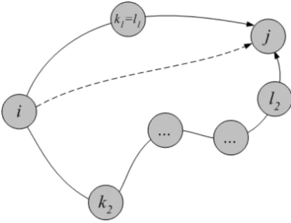
Fig. 4. Load-balancing example illustrating Proposition 12. The dashed line betweeniandjis a direct path. The two other paths are load-balanced paths inPLB(i, j). In the first load-balanced pathk1=l1, in the secondk2=l2.
APPENDIXII
OPTIMALITY OF THEBIASEDMESH(PROPOSITION7) In this Appendix, we will prove that the biased mesh achieves the maximum possible guaranteed throughput for any possible admissible capacity matrix by establishing Proposi-tion 7. To do so, we will first prove several useful Lemmas and Propositions by considering rate matrices that are also permutation matrices.
A. Throughput Bounds over the Set of Permutation Rate Matrices
It helps to study how the load-balancing is done. Let the set ofload-balanced paths
PLB(i, j) ={p∈P(i, j) : (i→j)∈p}
be the set of paths p between nodes i and j such that the link i → j is not in p. We will call paths not in PLB(i, j)
direct paths. For instance, 1→3→2is a load-balanced path between node 1 and node 2, whereas 1 →2 and 1 →1 → 2→2are direct paths.
Proposition 12: Any path p∈ P(i, j) satisfies one of the following two cases:
(i) Ifpis a direct path then(i→j)∈p, or
(ii) Ifpis a load-balanced path then there exist two nodesk
andl, possibly equal, such thatk=i,k=j,l =i and
l=j, such thatpcontainsi→k andl→j.
Proof: (i) clearly follows from the definition of
PLB(i, j). In (ii), by definition ofPLB(i, j), at least one node
is different from i, and if node k is the first node in path p
that is different fromi, then k=j also. Similarly, if node l
is the last node in pathpthat is different from j, then l =i
also.
Using this characterization of load-balanced paths, we con-sider all the rate matrices that are also permutation matrices, such that each node sends all its traffic to some other node. For a permutationσ, let
S1(σ) ={i:σ(i) =i}
denote the set of nodes invariant toσ, and let
denote the remaining nodes. The following lemma proves a general upper bound on the throughput θ(C)by considering the set of rate matrices that are permutation matrices.
Lemma 13: Given a capacity matrix C, the throughput
θ(C) has the following upper bound taken over the set of permutations: θ(C) ≤ 1 2+ 1 2N × min σ permut. i∈S1(σ) Cii+ i∈S2(σ) (Ciσ(i)−Cii)
Proof: By definition of the throughput θ(C), for any permutation σ,
θ(C)≤θ(C, σ).
Therefore, we only need to show that for any permutation σ,
θ(C, σ)≤1 2 + 1 2N i∈S1(σ) Cii+ i∈S2(σ) (Ciσ(i)−Cii) .
Consider a given permutation σ. By definition of θ(C, σ), any nodeimanages to send traffic at rateθ(C, σ)to nodej= σ(i). (We know that the optimum can be reached because the throughputθis defined using continuous functions on compact sets.)
Consider then a path p between i and j = σ(i), and distinguish between the following cases.
1) Ifp∈PLB(i, j), then from Proposition 12,pcontributes
at leastTijp toCij.
2) Ifp∈PLB(i, j), then by Proposition 12 there exists two
nodesk andl such that k=i,k= j, l=i andl=j, and such that p contains i → k and l → j. Hence, p
will use a rate of at leastTijp out of the capacityCikin
order to carry the linki →k, and will also use a rate of at least Tijp out of the capacityClj in order to carry
the linkl→j.
Therefore,prequires a total rate of at least2·Tijp from the non-diagonal elements of the capacity matrixC. These two cases show that the link between i and j = σ(i)can use non-diagonal capacity both with direct and load-balanced paths.
In particular, the first case studies thedirectpaths. It shows that the link between i and j = σ(i) uses a rate of at least
p∈PLB(i,σ(i))T
p
iσ(i) out of Ciσ(i) for the direct paths. This
is a contribution to the non-diagonal capacity if and only if
σ(i)=i, i.e.,i∈S2(σ). Also, since the capacity for the direct link should be greater than its rate in order to be feasible, we get
Ciσ(i)≥
p∈PLB(i,σ(i))
Tiσp(i). (8)
The second case studies the load-balanced paths. It shows that the link between i and j = σ(i) uses a rate of at least
p∈PLB(i,σ(i))2·T
p
iσ(i) out of the non-diagonal elements of
C for the load-balanced paths.
As a feasibility condition, the sum of the capacities of all the non-diagonal links should be more than the sum of all the
rates required from these non-diagonal links. Therefore, using the two cases studied above, we get
non-diagonal capacity≥non-diagonal required rate,
i.e., i,j=i Cij ≥ i∈S2(σ) p∈PLB(i,σ(i)) Tiσp(i) + N i=1 p∈PLB(i,σ(i)) 2Tiσp(i).
We now study the two sides of this equation. On the left hand side, sinceC is admissible, we have
N− i Cii≥ i,j=i Cij.
On the right hand side, the sum of all the rates required from these non-diagonal links can be rewritten as
i∈S2(σ) p∈PLB(i,σ(i)) Tiσp(i) + N i=1 p∈PLB(i,σ(i)) 2Tiσp(i) + p∈PLB(i,σ(i)) 2Tiσp(i) − N i=1 p∈PLB(i,σ(i)) 2Tiσp(i) = 2N θ(C, σ)−2 i∈S1(σ) p∈PLB(i,σ(i)) Tiσp(i) − i∈S2(σ) p∈PLB(i,σ(i)) Tiσp(i),
usingT =θ(C, σ)·σ andS1(σ)∪S2(σ) ={1, ..., N} in the
last equality. Using Equation (8), the sum of the non-diagonal rates can therefore be lower bounded by
2N θ(C, σ)−2 i∈S1(σ) Ciσ(i)− i∈S2(σ) Ciσ(i).
Finally, we combine the equations and use the definition of
S1(σ):i∈S1(σ)iffσ(i) =i. We get N− i Cii≥2N θ(C, σ)−2 i∈S1(σ) Cii− i∈S2(σ) Ciσ(i). Therefore, θ(C, σ)≤ 1 2+ 1 2N i∈S1(σ) Cii+ i∈S2(σ) (Ciσ(i)−Cii) .
B. Throughput Upper-Bound for a Capacity Matrix
We will now provide an upper-bound for the throughput of a capacity matrix by considering specific permutations. For
0 ≤ k ≤ N−1, define the permutation σk as the kth
sub-diagonal, i.e., assume that node i destines all its traffic to
σk(i) =i+kmodN. We can then apply Lemma 13 to find the
upper bound corresponding to each permutation, as expressed in the following lemma.
Lemma 14: Given a capacity matrix C, the throughput
θ(C)has the following upper bounds:
θ(C)≤1 2 + N i=1Cii 2N , (9) and θ(C)≤1 2 +min1≤k≤N( N i=1(Ci(i+kmodN)−Cii)) 2N . (10)
Proof: Fork= 0,S1(σk) ={1, ..., N}, hence the
upper-bound from Lemma 13 is 12 +
N
i=1Cii
2N . Similarly, for 1 ≤
k ≤N−1,S2(σk) ={1, ..., N}, hence this upper-bound is
1 2+
N
i=1(Ciσk(i)−Cii)
2N .
Proposition 15: If the capacity matrix C is admissible, i.e., C is a doubly sub-stochastic matrix, then its throughput satisfies
θ(C)≤ N 2N−1.
Proof: We will prove this by contradiction. Suppose that
θ(C)> N 2N−1. For0≤k≤N−1, let xk= N i=1 Ci(i+kmodN).
It follows from (9) and (10) that
x0> N 2N−1, (11) and for k= 1,2, . . . , N−1, xk−x0> N 2N−1. (12)
Therefore, we have xk > 2N2N−1 for k = 1,2, . . . , N −1.
Summing up for all kyields
N < N−1 k=0 xk= N i=1 N j=1 Ci,j.
This contradicts the assumption that the capacity matrix C is a doubly sub-stochastic matrix.
As the biased mesh with capacity matrix Cˆ achieves the throughput N/(2N −1), it then follows from Proposition 15 that the biased mesh is optimal among all the admissible capacity matrices.
APPENDIXIII
UNIQUENESS OF THEOPTIMALCAPACITYMATRIX (PROPOSITION8)
In this Appendix, we will prove that the biased mesh is the only capacity matrix that achieve the optimal throughput
N/(2N − 1), and therefore we will be able to establish Proposition 8.
Lemma 16: If an admissible capacity matrixCachieves the optimal throughput N/(2N−1), then the capacity matrix C
satisfies N i=1 Cii = N 2N−1, (13) and fork= 1,2, . . . , N−1, N i=1 Ci(i+kmodN)= 2 N 2N−1. (14)
Proof: As in the proof of Proposition 7, let
xk = N
i=1
Ci(i+kmodN).
If an admissible capacity matrix C achieves the optimal throughputN/(2N−1), then we have from (9) and (10) that
x0≥ N 2N−1, (15) and fork= 1,2, . . . , N−1, xk≥ 2 N 2N−1. (16)
If one of the inequalities in (15) and (16) is strict, then
N−1
k=0 xkwill be strictly larger thanNand this will contradict
to the assumption thatCis admissible. Therefore, we conclude that all the inequalities in (15) and (16) are in fact equalities. Lemma 17: If an admissible capacity matrixCachieves the optimal throughputN/(2N−1), then for any permutation σ,
i∈S2(σ)
(Ciσ(i)−2Cii) = 0.
Proof: Equation (13) in Lemma 16 provides
i∈S1(σ)Cii +
i∈S2(σ)Cii = N/(2N − 1) for any
permutationσ. Hence, using Lemma 13, we get
N 2N−1 ≤ 1 2 + 1 2N minσ N 2N−1 + i∈S2(σ) (Ciσ(i)−2Cii) ,
where the minimum is taken over the set of permutation matrices. Therefore, 0≤min σ i∈S2(σ) (Ciσ(i)−2Cii) ,
i.e., for any permutationσ,
0≤
i∈S2(σ)
(Ciσ(i)−2Cii).
We now use the fact that there are exactly (N − 1)!
permutations σ such that σ(i) = j for any nodes i and j. As a consequence, given a nodei, there are exactly(N−1)!
permutations σ such thati∈S2(σ), i.e., such thatσ(i) =i. Therefore, there are exactly N!−(N −1)! permutations σ
such that i∈S2(σ). We can deduce that σ i∈S2(σ) (Ciσ(i)−2Cii) = (N−1)! i,j=i Cij−2(N!−(N−1)!) i Cii = (N−1)! i,j Cij−(2N!−(N−1)!) i Cii =N!−(N−1)!·(2N−1)· N 2N−1 = 0,
where we use (13) in the last equality. Therefore, given that the sum of all these numbers is 0, and that they were all shown to be nonnegative, this means that they are all null.
The next lemma enables us to determine the exact value of the diagonal elements of C.
Lemma 18: If an admissible capacity matrixCachieves the optimal throughput N/(2N−1), then for alli,
Cii = 1
2N−1.
Proof: Pick arbitrarily any node — for instance, node
1 without loss of generality. For any node j = 1, consider the permutation σ such that σ(1) = j, σ(j) = 1, and the restriction ofσto the other elements is the identity. By Lemma 17, C1j+Cj1 = 2(C11+Cjj). Summing over all such j’s
yieldsNj=2(C1j+Cj1) =
N
j=22(C11+Cjj). Adding2C11
on each side of the equation and using (13) and (14) yields
1 + 1 = 2(N−1)C11+ 2
N 2N−1.
HenceC11= 2N1−1. Since we picked the first node arbitrarily,
this is similarly true for any node.
Proposition 19: The only matrix C that can achieve the optimal throughputN/(2N−1)is the capacity matrixCˆ from the biased mesh.
Proof: Combining Lemmas 17 and 18, for any permu-tation σ, i∈S
2(σ)Ciσ(i) = (2· |S2(σ)|)/(2N −1), where |S2(σ)|denotes the number of elements inS2(σ).
Define matrixDsuch thatDij =Cij fori=j, andDii=
2/(2N−1) = 2Cii. Then all row and column sums of Dare
equal to1 + 1/(2N−1)(becauseC is doubly stochastic). In addition, for any permutation σ,
i Diσ(i) = i∈S1(σ) Diσ(i)+ i∈S2(σ) Diσ(i) = i∈S1(σ) Dii+ i∈S2(σ) Diσ(i) = 2· |S1(σ)| 2N−1 + 2· |S2(σ)| 2N−1 = 2N 2N−1.
Hence, any permutation on D has the same sum! For any two nodes i, j, construct two permutations equal everywhere except on{D11, Di1, D1j, Dij}. ThenD11+Dij =Di1+D1j.
Therefore, all elements of D can be written as Dij =Di1+
(D1j −D11) = ui+vj, where u andv are two sequences
defined on {1, ..., N}. Since all row and column sums of D
are the same, all elements ofD are equal; therefore, all non-diagonal elements of C are equal, and finallyC= ˆC.
Therefore, we have finally established Proposition 8. APPENDIXIV
LOAD-BALANCINGGAIN(PROPOSITION11) We will now prove the equation in Proposition 11.
Proof: The right-hand-side of the equation comes directly from Proposition 10. The left-hand-side results from using the uniform mesh instead of the biased mesh to create the lower bound in Proposition 10. If Cunif orm is the uniform mesh,
θ(Cunif orm) = 1/2 and Cunif ormij = 1/N, therefore their