Stock Returns and the Dispersion in Earnings Forecasts

Department of Economics

Working Paper No. 0117

http://www.fas.nus.edu.sg/ecs/pub/wp/wp0117.pdf

Stock Returns and the Dispersion in Earnings Forecasts

Cheolbeom Park

Abstract: This paper derives a negative relationship between the dispersion of forecasts among investors and future stock returns based on Harrison and Kreps (1978). Using monthly data for earnings forecasts by market analysts, this paper presents empirically that the dispersion in forecasts has particularly strong predictive power for future stock returns at intermediate horizons (between 25 months and 44 months). The direction of predictive power from the dispersion for future stock returns is consistent with the derived negative relationship. Further, results suggest that the dispersion in forecasts contains information about future stock returns aside from the information contained in other variables.

JEL classification: E44, G10, G12

© 2001 Cheolbeom Park, Department of Economics, National University of Singapore, 1 Arts Link, Singapore 117570, Republic of Singapore. Tel: (65) 874 6015; Fax: (65) 775 2646; Email: ecscp@nus.edu.sg. This paper is based on a chapter of my Ph. D. dissertation at the University of Michigan (Park (2001)). I am especially grateful to Robert Barsky and Matthew Shapiro for their encouragement, guidance, comments and discussions. I thank Lutz Kilian, E. Han Kim, Dmitriy Stolyarov and seminar participants at National University of Singapore, University of Michigan, and University of New Hampshire for helpful comments and discussions. I also thank I/B/E/S Inc. for providing the data used in this paper. However, all remaining errors are mine. Views expressed herein are those of the author and do not necessarily reflect the views of the Department of Economics, National University of Singapore

I. Introduction

The efficient market hypothesis based on homogeneous expectations implies that future stock returns are unpredictable. Furthermore, this hypothesis also implies that unexpected movements of stock prices must be interpreted in terms of unexpected news about future dividends. However, the excess volatility of stock prices and the forecastability of stock returns have been well documented in an extensive literature. For example, Shiller (1981), and Campbell and Shiller (1988a, 1988b) reported that the stock market is too volatile to be explained by movements of dividends. Also, Fama and French (1988), Campbell (1991), Campbell, Lo and MacKinlay (1997), and Lamont (1998) showed that financial variables such as the relative Treasury bill rate and the ratios of price to

dividends, price to earnings, or dividends to earnings have predictive power for future movements of stock returns. Although economists have not yet reached a consensus on the source of these two puzzles −excess volatility and the forecastability of stock returns− one possible answer might be that financial markets are indeed inefficient.

This paper adds to the body evidence supporting the predictability of stock returns by showing that the dispersion in earnings forecasts by analysts also has a predictive power for future stock returns and that the predictive power is not a proxy of other popular forecasting variables. In other words, the dispersion in expectations among market analysts varies over time and has predictive power for future stock returns. This finding not only provides another piece of evidence that stock returns are predictable, but also points to alternative models to explain the movements of stock prices. Instead of attributing the predictive power of the dispersion in forecasts to market inefficiency, this

paper argues that the predictive power from the dispersion in forecasts can be explained by speculative interaction among investors holding heterogeneous expectations.

Keynes (1936) argued that the pursuit of gains from speculative trading is the main motivation for individual investors and that investors are interested in other investors’ expectations in order to gain from resale.1 Harrison and Kreps (1978) later showed that investors pursue gains from resale when they are aware that other investors have different opinions about future variables.2 Furthermore, they demonstrated that willingness to pay by investors will deviate from their own present value of future dividends because of the expected gains from resale in the future. This paper extends Harrison and Kreps’ implication by relating the difference between each investor’s willingness to pay and his or her expected present value of future dividends to the

average divergence in expectations across investors. From the point of view of Keynes or Harrison and Kreps, therefore, the predictability of the dispersion may not be so

surprising because the dispersion itself shows the average extent to which different expectations are held across investors.

At an intuitive level, it is easy to understand why the dispersion in forecasts can convey information that is valuable for speculative trading, when one uses a simple demand and supply model. One reason might be that as investors’ forecasts become more diverse, investors usually perceive greater gains from resale because there will be an increase in the number of optimistic investors. In this paper, this effect will be called the

1 _{Keynes’ view of the role of speculation is presented in Keynes (1936, Chapter 12).}

2 _{There are recent researches showing evidence for heterogeneous expectations. Using micro survey data}

for exchange rates, Ito (1990) showed not only that market participants’ expectations violate the rational expectation hypothesis but also that they have heterogeneous expectations stemming from individual effects. More interestingly, using almost the same micro survey data for exchange rates, Elliot and Ito (1999) showed that a simple trading strategy based on the prediction in the survey data can create average

‘demand effect’.3 Whenever investors have speculative motivations, hence, the dispersion will exert its own systematic effect on demand in the market and cause stock prices to change. As a result, part of the movements of stock prices can be explained by the dispersion in forecasts.

Section II briefly summarizes Harrison and Kreps’ model. I then extend their model to derive a prediction on the relation between the dispersion in expectations and future stock returns. With plausible assumptions from the data such as stationarity of the dispersion, this paper shows that current high dispersion predicts relatively low stock returns in the future.

Section III discusses how to measure the dispersion and reports summary statistics for the dispersion. In order to measure the dispersion in forecasts across

investors, I/B/E/S data is used. I/B/E/S is a Wall Street research firm providing forecasts for the aggregate S&P 500 earnings per share every month. Section III addresses two further issues: whether the dispersion in expectations has any predictive power for future stock returns, and whether it contains information aside from that contained in other variables used to forecast future stock returns. The first issue is studied via long-horizon regressions using a measure of dispersion, rather than other financial indicators such as price-to-dividend ratio. Interestingly, the dispersion seems to have particularly strong predictive power for future stock returns at intermediate horizons (from 25 months to 44 months). The coefficient of the dispersion variable in the regression is significantly negative and the dispersion appears to explain up to 14% of the movements of future

positive profits, although the predictions in the survey data do not satisfy the conditions for the rational expectations hypothesis.

3 _{One can think of the ‘supply effect’ resulting from additional supply created by short sales of pessimistic}

stock returns during these horizons.4 Regarding the second issue, the predictive power of the dispersion is not spurious. In other words, the dispersion is not a simple proxy for other popular forecasting variables, such as the relative Treasury bill rate and the ratios of price to dividends, price to earnings, or dividends to earnings. The dispersion also has the ability to predict future stock returns even when standard macroeconomic variables, such as the growth rate of industrial production, the inflation rate, and the interest rate are included in the long-horizon regression. In addition, an explanation for strong predictive power at intermediate horizons is provided in Section III.

Section IV examines what moves the dispersion in earnings forecasts to see more directly whether the dispersion is a proxy for other variables and to check whether the results in the previous section are robust. This section shows that most of the movements cannot be explained by market volatility, financial forecasting variables, macroeconomic variables, or major non-economic news events such as elections and international

conflicts.

Section V investigates potential finite sample biases in long-horizon regressions via Monte Carlo simulation. The results in this section show that the finite sample bias appears to be not serious enough to reject the results in Section III. Finally, some concluding remarks are offered in Section VI.

II. A Model for the Predictive Power of Dispersion

In this section, I demonstrate that the dispersion in forecasts has a direct effect on the demand for stocks. Since better opportunities for resale gains occur when the dispersion

4 _{The negative coefficient for the dispersion is another piece of evidence that the demand effect dominates}

becomes greater, the dispersion can affect the demand and can forecast future movements of stock prices. In this section, the role of dispersion in the demand effect is more

precisely and more explicitly articulated, based on Harrison and Kreps (1978). This section, then, investigates how dispersion can provide information on future movements of stock prices.

Harrison and Kreps (1978) modeled heterogeneous expectations across investors by simply assuming that investors have different subjective probability assessments. Under additional assumptions that no short sales are allowed and that each internally homogeneous class has infinite collective wealth, they showed that the equilibrium stock price will be the maximum willingness to pay across investors.5 Furthermore, they proved that in their model, to obtain any potential gains from resale, the optimal investment strategy for every investor is the strategy that buys, holds for only one period, and then resells. Since the optimal decision rule requires investors to be interested in only next period’s dividends and resale prices, one can define each individual investor’s

willingness to pay denoted by a( _i)

t s p , as ] | [ ) ( _{i t}a _{t 1 t 1 t i} a t s E d p S s p = γ ₊ +γ ₊ = (1) where a is a class of investors who have identical expectations, γ is the discounting rate,

t

d is the dividends paid at time t and S_t =s_i denotes the state of the level of dividends being paid at time t. Given this result, it is straightforward to write the equilibrium stock prices as

[

]

5 _{Harrison and Kreps (1978) excludes the supply effect by the assumption of no short sales in the stock}

Although Harrison and Kreps already noted that equation (1) is greater than

∑

E _γ in general and that the difference between equation (1) and

∑

E γ was due to the consideration of the gains from resale, they did not show explicit economic implications. However, if one uses equation (1) and (2) recursively, then every individual investor’s willingness to pay can be rewritten as

] | [ ) ( a _{t 1 t 1 t i} t i a t s E d p S s p = γ ₊ +γ ₊ =

∑

∑

It is important to note here that an individual investor’s willingness to pay is no longer the present value of future dividends. More importantly, however, the difference between ]p_ta(s_i)=E_ta[γd_t+1+γp_t+1|S_t =s_i and

∑

to the expected present value of future gains from resale. In fact, this difference results from the fact that investors have the right to resell stocks in the future. Furthermore, as long as an investor has a state in which he or she is not the most optimistic investor, the expectation of future standard deviation in willingness to pay across investors will be a factor that affects the investor’s willingness to pay.

Suppose that the number of heterogeneous classes in an economy is constant at N. Then, since the future equilibrium price will be the maximum of N random drawings from the distribution of willingness to pay across investors, an investor’s willingness to pay becomes greater for most distributions as the investor expects higher standard

deviation in the future.6 Intuitively, the reason is that the expected maximum of N random drawings from a distribution has positive relationship with the expected standard

deviation. For example, when investors’ expectations are approximately normally distributed, one can clearly see this argument. With a normal distribution for willingness to pay, equation (3) can be rewritten as

∑ = + ∑ − = = ∞ = ∞ = + + + 1 1 ] | ) ( [ ] | [ ) ( j j t j t i a j t j a t i t j t j a t i a t s E d S s E Z Z S s p _{γ γ σ} (4)

where Z is the constant expected maximum of N random drawings from the standard normal distribution, a

t

Z is a constant that reflects the individual investor’s relative position in the standard normal distribution and _σt is the standard deviation of the willingness to pay across investors.7 Thus, the expectation of σ_t affects individual investors’ willingness to pay and the equilibrium price eventually.

If σ_t has a positive relation with the dispersion in one-year ahead earnings forecasts, then one can obtain explanations for the demand effect and the predictive power from the dispersion. If the dispersion in earnings forecasts denoted by σ_t is positively serially correlated, the demand effect will exist.8 If current σt is high, then it

will raise the expectations of future _σt and as a result, every investor’s willingness to pay will become higher. In other words, investors will perceive greater gains from

6 _{Park (2001) examines the demand and the supply effect at the same time by allowing short sales in the}

stock market. If the fraction of stockholders to all potential investors is constant and if the fraction is small due to high costs in short sale, then one can also derive the same empirical implication. See Park (2001).

7 _{Even if one assumes a different distribution for the willingness to pay across investors rather than normal}

distribution, one can still show that the second term in equation (2) has a positive relation with the standard deviation of the non-normal distribution in most cases.

speculative trading as σ_t becomes greater. Since willingness to pay of all investors becomes higher, stock prices will rise.

Then, how can σ_t predict future stock returns? Suppose that every investor believes that σt follows a stationary process.9 If current σt is unusually high, then the

current stock price will be higher than normal because of the demand effect. As _σt returns to its normal level, however, the demand effect will weaken and stock prices will fall, all other things held constant. This effect will become more evident as time goes on. As a result, a high σ_t in the current period implies relatively low future stock returns and vice versa. Therefore, part of the movements in stock prices might be explained by the movements of dispersion, and this possibility will be examined in the next section.10,11

III. Forecastability of Dispersion

This section discusses how to measure the dispersion in one-year ahead earnings forecasts and shows summary statistics for the dispersion. It then addresses the issue of whether the dispersion in expectations has any predictive power for future stock returns and the issue of whether it contains information aside from the information contained in other variables used in forecasting future stock returns. A brief interpretation of the empirical results based on the model presented in the previous section will also be offered.

9 _{Stationarity in}

t

σ seems realistic given the data. See Table 1 of this paper.

10 _{In contemporaneous but independent research, Chen, Hong and Stein (2001) and Scherbina (2001) derive}

an identical implication using Miller’s (1977) conjecture. In order to derive a negative relationship between the dispersion and future stock returns based on Miller’s conjecture, however, one important assumption is that the median forecast should be the correct assessment for future fundamentals although Harrison and Kreps’ (1978) interpretation does not require this assumption.

A. Data and Construction of Variables

The dispersion in this paper is defined as the coefficient of variation in analysts’ earnings forecasts, which is the ratio between the standard deviation and mean of earnings

forecasts. The reason to normalize the standard deviation by the average is to exclude the effect that the standard deviation increases with the average. Thus by definition, the dispersion is independent of the inflation rate.

The average and standard deviation in the earnings forecasts for the S&P 500 index are taken from the I/B/E/S dataset. I/B/E/S is a Wall Street research firm that collects forecasts for individual company earnings for current and subsequent fiscal years from stock market analysts every month. I/B/E/S specifically asks for forecasts of

operating earnings per share, which excludes non-recurring or unusual expenses or income such as restructuring costs or unusual capital gains or losses.

I/B/E/S has reported forecasts of the aggregate S&P 500 earnings per share in current, denoted here by EPS1, and the forthcoming (EPS2) calendar years since January of 1982. Forecasts of the aggregate S&P 500 earnings for any given calendar year are constructed monthly beginning in March of the previous year. As a result, the forecast horizon becomes shorter as the calendar year progresses. For example, in March of each year the maximum forecast horizon is almost two full years, whereas in February, the maximum forecast horizon is only 10 months. In order to take advantage of the monthly frequency of the forecast data, however, this paper uses some approximations to construct the dispersion of 12-month ahead earnings forecasts (_σt), that is:

11 _{Recent researches on the cross-sectional examination of this implication are Chen, Hong and Stein}

1) σ_t=

2 2

AF SD

for December, the following January and February

2) σt = 2 1 2 1 * * ) 1 ( ) 1 ( AF w AF w SD w SD w AF SD m m m m − + − +

= for March – November

where AF₁ (SD₁) is the average (standard deviation) of EPS1, AF₂ (SD₂) is the average (standard deviation) of EPS2, and w_m is 9/12 in March, 8/12 in April, and so on, ending at 1/12 in November.

Except for the average and standard deviations in earnings forecasts data, all the data used here (e.g., the S&P 500 monthly price index, S&P 500 monthly dividend yield, S&P 500 monthly price-earnings ratio, monthly consumer price index, industrial

production, Treasury bill rates, money stock measured as M1 and Moody’s AAA corporate bond yield) are from the DRI database.12 Constructing monthly real stock returns for the aggregate S&P 500 and calculating financial indicators such as the ratios of price to dividends, price to earnings, or dividends to earnings between January 1982 and October 2000 are straightforward.

Figure 1 shows the movements of monthly real stock returns for the S&P 500, dispersion (_σt) and the average forecast. Table 1 also reports summary statistics of _σt along with other popular forecasting variables. Popular forecasting variables are other variables reported elsewhere as containing predictive power for future stock returns. Fama and French (1988), Campbell and Shiller (1988a, 1988b), and Campbell, Lo and MacKinlay (1997) all find that the ratios of price to dividends or earnings have strong

12 _{The DRI codes for each data series are as follows. The DRI code for the S&P 500 monthly price index is}

FSPCOM, the code for the S&P 500 monthly dividend yield is FSDXP, the code for the S&P 500 monthly price-earnings ratio is FSPXE, the code for monthly consumer price index is PUNEW, the code for industrial production is IP, the codes for Treasury bill rates are FYGM3, FYGM6 and FYGMYR, the code

predictive power for future stock returns. Lamont (1998) shows that the log payout ratio (log dividends to earnings ratio) performs well in predicting stock returns. Campbell (1991) reports that the relative Treasury bill rate is a good forecasting variable for stock returns.

As shown in Table 1, the autocorrelation of _σt is fairly high but substantially lower than unity (0.66) and the null hypothesis that _σt contains unit roots can be rejected at a conventional significance level. Thus, the use of σ_t in the following long-horizon regressions does not create a potential inference problem, which could arise if an

econometrician used the other variables, since these are very persistent and contain roots extremely close to unity. In addition, the correlations of _σt with other popular

forecasting variables are relatively lower than among the other forecasting variables themselves, which may imply that if _σt has a predictive power on future stock returns, then the reason may be different from those for other predictors.

The sample periodogram of _σt is also provided in Figure 2, which displays )

(

ˆ _j

s_{σ ω} , the sample periodogram, as a function of j, frequency, where _{ω =j} 2_πj/T and T is the sample size. As shown in Figure 2, one can find peaks at least two frequencies. In addition to the large contribution of the second lowest frequency (j = 2) to the variation of

t

σ , there is a peak occurring around j = 8, which explains a relatively higher portion of the variation in the dispersion. Interestingly, the peak around j = 8 corresponds to a cycle with a period of 28 months. An additional seasonal effect in the dispersion may be

for money stock measured as M1 is FM1 and the code for Moody’s AAA corporate bond yield is

detected from the peak around j = 21 because this peak corresponds to a period of 11 months.

B. Long-horizon Regression with Dispersion

One easy and popular way to judge the predictive ability of a variable on future stock returns is to check the significance of the coefficient of the variable and the _R2 _in

long-horizon regressions.

Table 2 shows the results of implementing long-horizon regression, using the dispersion in earnings forecast (_σt) as a regressor. Over the sample period covered in this paper, the dispersion (the coefficient of variation for the S&P 500 earnings forecasts in I/B/E/S data set) seems to have predictive power for future stock returns at

intermediate horizons (from a 25-month horizon to 44-month horizon). During these horizons, the coefficient of the dispersion in the regression is significantly negative, and the dispersion in forecasts alone appears to explain up to 14% of the movements of future stock returns. Furthermore, the predictive power from σ_t looks hump-shaped. The significance of the coefficient of _σt and _R2 _{both first increase with the length of the}

horizon but then begin to decline around 34 months and 30 months, respectively. The results presented here are not subject to the potential inference problems that arise with other popular predicting variables which have roots much closer to unity.

Since σ_t is the ratio between the standard deviation and average of earnings forecasts, one might doubt whether the predictive power of σt comes from the average.

k t t t t k t t r a b b af p r₊₁+_L+ ₊ = ₀ + ₁σ + ₂( − )+ε ₊ (5) where r is the log real return, and af_t −p_t is the log average forecast-price ratio. The log average forecast-price ratio is used to eliminate any possible nonstationary component in the average earnings forecast. The results are reported in Table 3. As shown in Table 3, the results in the previous table do not appear to originate from the predictive power of the average earnings forecast. Even with af_t − p_t, the incremental _R2 _{due to}

t

σ 13 _is

significant at the intermediate horizons and the coefficient for _σt is also significantly negative from 25-month horizon to 38-month horizon while the coefficient for af_t − p_t is never significant until 48-month horizon. In addition, the predictive power of σt in terms

of the significance of the coefficient for _σt or incremental _R2 _{due to}

t

σ also looks hump-shaped.

Another issue to address is whether the dispersion in earnings forecasts contains any incremental information about future movements of stock returns aside from the information contained in other available variables. In order to investigate this possibility, the following regression is run

k t t t k t t r a Z b r₊1+L+ ₊ = 0 +γ + σ +ε ₊ (6)

where Zt is composed of all the popular forecasting variables in the previous sub-section

in order to examine whether the dispersion really provides additional information with regard to future stock returns.14

13 _{The incremental R}2 _{due to}

t

σ is the difference between the _R2 _{when both}

t

σ and af_t−p_t are used as regressors and the _R2 _{when only}

t

t p

af − is used as a regressor.

14 _{Obviously the log dividend price ratio, the log earnings price ratio and the log dividend earnings ratio}

cannot be included in the regression at the same time because of the multicolinearity problem. Hence, I run two regressions. The log dividend price ratio, the log dividend earnings ratio, the relative Treasury bill rate

The regression results with one change of variable, are given in Tables 4 and 5. As the results are almost identical, henceforth this paper will concentrate on the results in Table 4. Even with other popular forecasting variables, the coefficient of the dispersion is significant between the 28-month horizon and 39-month horizon. Furthermore, from the 6-month horizon, the incremental _R2 _{of the regression due to}

t

σ is positive and _σt adds up to almost 8% of the explanatory power. Like the previous regression results, _σt seems to have hump-shaped predictive power.

In addition, the results shown in Table 4 have another interesting feature. The log dividend earnings ratio has remarkable predictive ability from the one-month horizon to the 30-month horizon. The good forecastability of d_t −e_t is consistent with Lamont (1998). The relative Treasury bill rate also has relatively good predictive power for future stock returns for horizons from one through 3 months, as reported in previous research (e.g. Campbell (1991)). However, _σt is the only variable that has significant coefficients between 34-month horizon and 39-month horizon.

Table 6 investigates whether the dispersion contains additional information relative to some macroeconomic variables such as the growth rate in industrial

production, the inflation rate and the interest rate. The monthly consumer price index is used to measure the inflation rate, and real three-month Treasury bill rate15 is used for the interest rate. In order to address this question, I run the following regression.

k t p t p t t k t t r a Z b b r₊1+L+ ₊ = 0 +γ + 1σ +L+ σ ₋ +ε ₊ (7) and the dispersion are the regressors for one regression and the log earnings price ratio, the log dividend earnings ratio, the relative Treasury bill rate and the dispersion are the regressors for the other regression.

where Z_t is a vector of current and lagged macroeconomic variables. The lag order is selected by Akaike information criterion.16 As shown in Table 6, the forecastability of the dispersion is little affected by the inclusion of common macroeconomic variables. F-statistics for current and lagged coefficients of _σt are significantly different from zero between the 23-month horizon and 42-month horizon, implying that _σt has additional information for future stock returns. The predictive power of σt also appears

hump-shaped.

In summary, the results in this section seem to show that σ_t has, to a

considerable extent, its own predictive ability for future stock returns. Furthermore, _σt has some incremental predictive power for future stock returns relative to some other forecasting variables or macroeconomic variables. The sign of the coefficient for σt in

long-horizon regressions is consistent with the earlier implication derived from Harrison and Kreps (1978). High σt in the current period raises current stock prices and implies

relatively low stock returns in the future because high _σt signals good opportunities for speculative resale.

In addition, the sample periodogram of _σt might be able to explain the hump-shaped feature of the predictive power, which seems at first sight to contradict the theoretical prediction that the effect from σt on future stock returns becomes more

evident as time passes. More precisely, the implication based on Harrison and Kreps’ model would predict that one might see a monotonically increasing predictive power of

t

σ in the length of horizons, if all other things are constant. However, the monotonicity

of the predictive power is likely to be destroyed by a cycle with a period centering on approximately 28 months because the peak around j = 8 explains a relatively higher portion of the variation in σt. Roughly speaking, this cycle corresponds to the horizon

when the predictive power from _σt begins to decline.

Thus, the findings in this section can be interpreted as evidence showing that the consideration for resale gains by investors holding heterogeneous expectations may affect stock prices. In the next section, I investigate what moves the dispersion, which appears to have considerable predictive ability for future stock returns.

IV. Causes of Dispersion Movements

If the dispersion in forecasts has considerable power to predict future stock returns, then what moves the dispersion? I address this question to determine more carefully whether the dispersion really contains its own information that cannot be explained by other variables and to check whether the results in the previous section are robust. Hence, this section investigates the relation between the dispersion and other variables that might cause the dispersion to fluctuate.

A. Dispersion and Market Volatility

Although there is no direct connection between stock market volatility and the dispersion in forecasts, these two concepts might be indirectly connected. There could be more disagreement among investors when an asset becomes more risky because market volatility normally reflects risk and uncertainty of an asset at each moment. Thus, it would be reasonable to suppose that the market volatility of stock returns would increase

as the dispersion in opinions increases. In other words, volatility and dispersion are expected to co-vary.

Although there are many ways to estimate volatility in the stock market, the volatility in this paper is estimated under ARCH (1), GARCH (1,1) and GARCH in Mean with AR (1) specifications, because GARCH-type models are widely used in financial economics since introduced by Engel (1982). Since one can obtain very similar volatility estimates under all specifications, the results in Table 7 are only shown for GARCH (1,1) specification.

As shown in Table 7, the conjecture that market volatility and dispersion in forecasts would co-vary does not seem to be supported by the data. Although the

volatility and dispersion have a positive correlation, the volatility does not Granger-cause the dispersion and the dispersion does not Granger-cause the volatility, either.

Furthermore, the current volatility can explain only about 2% of the movements of the dispersion while its coefficient is significantly different from zero. The R2 does not increase much even when lagged and future market volatility are included in the

regression equation. Using lagged, current and future market volatility together appears to explain about 6% of the variation in _σt. Therefore, the conjecture that the dispersion may reflect the volatility in the market cannot, at this stage, be accepted.

B. Dispersion, Forecasting Variables and Macroeconomic Variables

Here I investigate whether other popular forecasting or macroeconomic variables used in the previous section can explain a significant fraction of the movements of the dispersion. Hence, the following regression is run

t t

t a γZ ε

σ = 0 + + (8)

where Z_t is a vector of either forecasting or macroeconomic variables. Macroeconomic variables include stock returns for the S&P 500, the growth rate of real dividend for the S&P 500, the growth rate of industrial production, the growth rate of real money, nominal long-term interest rate measured as Moody’s AAA corporate bond yield, nominal short-term interest rate measured as the yield on three-month Treasury bill, CPI inflation rate, and volatility estimates in the previous sub-section.

The results are presented in Tables 8 and 9. Some conclusions emerge from these tables. First, neither current financial forecasting variables nor current macroeconomic variables are able to explain most of the movements in dispersion; in fact, forecasting variables and macroeconomic variables can explain about 6% and 9% of the movements, respectively.

Second, one can find variables that have relatively better explanatory power than other variables. The incremental R2 due to dt − pt or et − pt is greater than the R2 due

to all other financial forecasting variables. Three-month Treasury bill rates and volatility estimates also have relatively good explanatory power.

Third, although it is hard to explain the movements in _σt based on forecasting or macroeconomic variables, σt does not appear to be an exogenously given variable.

Several bivariate Granger-causality tests show that e_t − p_t, three-month Treasury bill rate and Moody’s AAA corporate bond yield Granger-cause _σt at a 5% significance level.

Finally, the explanatory power from either forecasting or macroeconomic variables has a great jump when two lagged variables are included in the regression

equation. This fact is more evident for the case of macroeconomic variables. If two or three lagged macroeconomic variables are included, then about one third of the movements in σt can be explained by these variables. Nevertheless, there remain

substantial unexplained movements in _σt.

In summary, although most movements of _σt cannot be explained by forecasting or macroeconomic variables, σt itself is not an exogenous or independent variable. One

can find other variables that Granger-cause _σt.

C. Major News and Dispersion

Besides volatility, forecasting or macroeconomic variables, political events and international conflicts can affect _σt. For example, international political tension immediately before wars often raises _σt while settlements of such conflicts lower _σt. Hence, this sub-section examines the relation between σt and major news events.17

First, the reaction of _σt to major non-economic events is investigated. Important non-economic events were identified using “Chronology of Events” from the World Almanac and Book of Facts. Further, events were excluded unless they were reported or discussed in the New York Times Business Section. Selecting major events in this way biases toward events that are expected to cause large swings in _σt.

Table 10 lists important events along with the percentage change in σ_t during the month.18 Although there are usually some gaps between days when events occurred and days when forecasts were made, some of the change in σ_t clearly appears to be

associated with the news. For example, as it became evident that the US would win the Gulf War, _σt had declined dramatically between January of 1991 and February of 1991. When the US was involved in conflicts with other countries, σt had always increased.19

However, the most surprising result is that the effects due to non-economic news are so small. While the standard deviation of the percentage change in σ_t for the whole sample is22.60%, the standard deviation of the percentage change in _σt during the month when such news occurred is merely 12.29%, even lower than that of the whole sample. Hence, it appears difficult to explain the movements of σt in terms of non-economic news

events.

Second, in order to identify the importance of news on the movements of σt,

high dispersion period20 and related news developments for each period are investigated. Table 11 shows the list of high dispersion periods. Although dispersions were generally high during recessions, it is still difficult to derive a relation between a high dispersion period and the release of economic or non-economic news. Especially, during the last two high dispersion periods (October 1992 – January 1993 and August 1999-December 1999), it is hard to identify relevant news items as contributing to the high dispersion.

18 _{Forecasts in I/B/E/S data are made on Thursdays that fall between the 14th and 20th of each month.}

Hence, events that happened between the 21st of the previous month and the 20th of the current month are assumed to affect current month forecasts.

19 _{Such events during the sample period are Korean passenger shot down by Soviet (Sep., 1983), US}

Marines killed in Lebanon and US invasion to Grenada (Nov., 1983), and US invasion to Panama (Dec., 1989).

Although there was turmoil in the European financial market in September of 1992, most news articles in the New York Times at that time analyzed that the turmoil in Europe had little serious impact on the US financial market. Another major news event during the period, Clinton’s election, does not appear to provide clear evidence for its role in maintaining high dispersion. Also, although one can find many articles expressing concerns about stresses from emerging markets during summer of 199921, there are some doubts whether this concern was the key source for the high dispersion during the last high dispersion period. However, it is interesting to note that the last high dispersion period coincides with the period when NASDAQ index kept rising rapidly. At the other extreme, _σt was very high immediately before the Gulf War broke out and this seems related with the war at that time. In conclusion, major news events do not seem to explain most of the movements in _σt and it is hard to establish a general relation between major news and movements in _σt.

This section has shown that most movements in σ_t cannot be explained by market volatility, other forecasting variables, macroeconomic variables, or major news events. This result implies more clearly that the predictive power of _σt is not a spurious proxy for these other variables.

V. Finite Sample Bias and Monte Carlo Simulation

It has been noted that there are two major pitfalls in applying the asymptotic theory to t-statistics in long-horizon regressions (Campbell, Lo, and MacKinlay (1997, Chapter 7)).

20 _{High dispersion period is defined as the period when dispersion stays higher than its mean plus one}

The first problem arises from the persistence of regressors in long-horizon regressions. It is a well-known fact that other forecasting variables such as the dividend price ratio are very persistent and seem to contain roots highly close to unity. Since the dispersion is not as persistent as other forecasting variables, this problem would not be as serious. The second problem arises from the fact that observations in the dependent variable of the long-horizon regression are overlapping. This problem would be serious especially when the horizon K is large relative to the sample size. The long-horizon regressions in this paper may have this problem. As a result, some finite sample biases appear to be unavoidable.

In order to examine possible finite sample biases in the long-horizon regressions in Section III, I conduct a Monte Carlo simulation. Under the null hypothesis that the coefficient of the dispersion is equal to zero, stock prices reflect the present value of future dividends. Hence, I generate artificial data for dividends, and then stock prices and stock returns are calculated from these generated dividends, according to Mankiw, Romer and Shapiro (1991). Since most movements of the dispersion cannot be explained by other variables, the artificial data for the dispersion are generated by the estimated coefficients under an autoregressive process. An AR(1) specification is selected for the dispersion process because Schwarz Criterion supports the AR(1) specification and because the first lagged dispersion (_σt−1) is the only variable that has consistently significant coefficients among AR(1) through AR(12).22 Innovations are bootstrapped from regression residuals under the AR(1) specification.

21 _{Stresses from emerging markets are currency problem and bank scandal in Indonesia, political mess in}

Russia, military tension in China and volatile stock market in Argentina.

As shown in Table 13, the finite sample bias becomes more serious with the length of horizon. The 5% critical value for t-statistics becomes greater in magnitude as the horizon increases. However, although Monte Carlo simulation indicates that the asymptotic distribution often leads to unreliable inference as the length of horizon increases, the distortion does not seem to be great enough to reject the previous results. Even with the simulated empirical distribution for t-statistics in the Monte Carlo

simulation, the actual t-statistics for the dispersion are greater in magnitude than the 5% critical values at intermediate horizons, which implies that the actual t-statistics obtained in the long-horizon regressions are very rare under the null hypothesis. Therefore, even taking into account of possible finite sample biases via Monte Carlo simulation, the null hypothesis that the dispersion has no predictive power for future stock returns can still be rejected at a conventional significance level.

VI. Conclusion

This paper has shown that the dispersion in earnings forecasts has its own predictive power for future stock returns. Furthermore, the dispersion measure contains information about future stock returns aside from the information contained in other variables. Also, most of the movements in dispersion cannot be explained by other variables such as popular financial indicators, macroeconomic variables, volatility, or non-economic events, which supports the robustness of incremental predictive power of _σt. Monte Carlo simulation additionally shows that finite sample biases in long-horizon regressions using the dispersion do not seem so serious.

Finally, the forecastability of σ_t can be explained by investors’ awareness of heterogeneity in expectaions, as described in Harrison and Kreps (1978). If investors are aware that other investors may have different expectations, then investors are interested in expectations by other investors to gain from speculation. In this sense, _σt carries information for opportunities of resale gains. Hence, currently high _σt implying better opportunities for resale gains raises stock prices in current period and lowers stock returns in the future.

Although the question of the source of heterogeneous expectations has not been fully addressed, some economists have recently begun to examine the consequences of differences in expectations among investors.23 In this kind of context, the results in this paper would seem to warrant a reconsideration of the previous rejection of the market efficiency hypothesis. In this study, although _σt has a forecasting ability for future stock returns, this ability appears to result from investors’ awareness of heterogeneity in beliefs rather than from market inefficiency. Hence, the results in this paper suggest a new direction for future research – investors’ awareness of heterogeneity in expectations need to be incorporated in any attempt to produce a fully adequate and explicative model for stock prices.

23 _{Hong and Stein (1999) also tries to explain price movements based on different opinions. There are also}

several recent papers focusing on the relation between trading volume and heterogeneous expectations. For example, see Bamber, Barron and Stober (1999).

References

Bamber, Linda S., Orie E. Barron, and Thomas L. Stober, “Differential

Interpretations and Trading Volume,” Journal of Financial and Quantitative Analysis, 34 (1999), 369-386.

Campbell, John Y., “A Variance Decomposition for Stock Returns,” The Economic Journal, 101 (1991) 157-179.

Campbell, John Y., Andrew W. Lo, and A. Craig MacKinlay, The Econometrics of Financial Markets, (Princeton: Princeton University Press, 1997).

Campbell, John Y., and Robert J. Shiller, “Stock Prices, Earnings, and Expected Dividends,” Journal of Finance, 43 (1988a), 661-676.

Campbell, John Y., and Robert J. Shiller, “The Dividend-Price Ratio and

Expectations of Future Dividends and Discount Factors,” Review of Financial Studies, 1 (1988b), 195-227.

Chen, Joseph, Harrison Hong, and Jeremy C. Stein, “Breadth of Ownership and Stock Returns,” Working paper, Stanford University (2001).

Cutler, David M., James M. Poterba, and Lawrence H. Summers, “What Moves Stock Prices?,” Journal of Portfolio Management, 15 (1989), 4-12. Elliot, Graham, and Takatoshi Ito, “Heterogeneous Expectations and Tests of

Efficiency in the Yen/Dollar Forward Exchange Rate Market,” Journal of Monetary Economics, 43 (1999), 435-456.

Engel, Robert F., “Autoregressive Conditional Heteroscedasticity with Estimates of the Variance of United Kingdom Inflation,” Econometrica, 50 (1982), 987-1007. Fama, Eugene F., and Kenneth R. French, “Dividend Yields and Expected Stock

Returns,” Journal of Financial Economics, 25 (1988), 23-49.

Harrison, J. Michael, and David M. Kreps, “Speculative Investor Behavior in a Stock Market with Heterogeneous Expectations,” Quarterly Journal of Economics, 92 (1978), 323-336.

Hong, Harrison, and Jeremy C. Stein, “Differences of Opinion, Rational Arbitrage and Market Crashes,” Working paper, Stanford University (1999).

Ito, Takatoshi, “Foreign Exchange Rate Expectations: Micro Survey Data,” American Economic Review, 80 (1990), 434-449.

Keynes, John M., The General Theory of Employment, Interest and Money, (Harcourt, Brace and Company, 1936).

LeRoy, Stephen E. and Richard D. Porter, “The Present Value Relation : Tests Based on Variance Bounds,” Econometrica, 49 (1981), 555-577.

Lamont, Owen, “Earnings and Expected Returns,” Journal of Finance, 53 (1998), 1563- 1587.

Mankiw, N. Gregory, David H. Romer and Matthew D. Shapiro, “Stock Market

Forecastability and Volatility: Statistical Appraisal,” Review of Economic Studies, 58 (1991), 455-477.

Miller, Edward, “Risk, Uncertainty and Divergence of opinion,” Journal of Finance, 32 (1977), 1151-1168.

Park, Cheolbeom, Movements of Stock Prices When Investors Have Different Expectations, Ph. D. dissertation, University of Michigan (2001).

Scherbina, Anna, “Stock Prices and Differences of Opinions: Empirical Evidence That Prices Reflect Optimism,” Working paper, Northwestern University (2001).

Shiller, Robert J., “Do Stock Prices Move Too Much to Be Justified by Subsequent Changes in Dividends?,” American Economic Review, 71 (1981), 421-436.

Table 1. Summary Statistics for the Dispersion (_σt) and Other Forecasting Variables

Univariate Summary Statistics

t t p d − et −pt dt −et rrelt σt Mean -3.56 -2.87 -0.69 -0.22 0.06 Standard Deviation 0.43 0.38 0.17 0.96 0.01 Autocorrela-tion 0.98 0.98 0.99 0.93 0.66 ADF test -0.64 -2.11 -0.80 -3.54 -3.61 Correlation Matrix t t p d − et −pt dt −et rrelt σt t t p d − 1.00 0.91 0.48 -0.35 -0.14 t t p e − 1.00 0.09 -0.39 -0.21 t t e d − 1.00 -0.02 0.13 t rrel 1.00 0.02 t σ 1.00

The sample contains monthly observations from January 1982 to October 2000. d_t − p_t is log dividend price ratio measured as the log difference between the sum of dividends paid on the S&P 500 index over the previous 12 months and the current level of the index. e_t −p_t is log earnings price ratio measured as the log difference between the sum of earnings obtained on the index over the previous 12 months and the current level of the index. d_t −e_t is log payout ratio (log dividend earnings ratio) measured as the log

difference between the sum of earnings and the sum of dividends paid on the index over the previous 12 months. rrelt is relative short term Treasury bill rate, which is the current

month’s Treasury bill rate minus its previous 12-month moving average. σt is the

coefficient of variation in earnings forecast. Autocorrelation is the first autocorrelation of each variable. ADF (Augmented Dickey-Fuller) test is t-statistics on _β in the regression

α ς

ς ∆ + + ∆ +

= t₋ p t₋p

t x x

x 1 1 _L +βxt₋1+et. Lag orders are selected by Ng and Perron

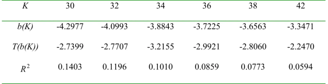
Table 2. Dispersion in Long-horizon Regression K 1 3 12 24 26 28 b(K) -0.0530 0.0707 -0.0588 -2.3941 -3.1818 -3.9010 T(b(K)) -0.3294 0.1827 -0.0637 -1.8126 -2.1921 -2.7534 2 R 0.0005 0.0002 0.0005 0.0528 0.0895 0.1257 K 30 32 34 36 38 42 b(K) -4.2977 -4.0993 -3.8843 -3.7225 -3.6563 -3.3471 T(b(K)) -2.7399 -2.7707 -3.2155 -2.9921 -2.8060 -2.2470 2 R 0.1403 0.1196 0.1010 0.0859 0.0773 0.0594

The sample contains monthly observations from January 1982 to October 2000. The regression equation is r_t+1 +L+r_t+K =a₀ +b(K)σ_t +ε_t+K,K where r is monthly log real returns on the S&P 500 index and _σt is the dispersion in forecasts (the ratio of standard deviation and mean earnings forecasts). T(b(K)) is the t-statistic using Newey and West (1987) standard errors. R2(K) is the R2 in the regression.

Table 3. Dispersion and Average Earnings Forecast in Long-horizon Regression K 1 3 12 24 26 28 ) ( 1 K b -0.0363 0.1667 0.2316 -2.3417 -3.1405 -3.8637 )) ( (b₁ K T -0.2155 0.4036 0.2410 -1.8306 -2.2050 -2.7044 ) ( 2 K b 0.0033 0.0191 0.0731 0.0249 0.0266 0.0228 )) ( (b₂ K T 0.4612 0.9937 1.2050 0.2643 0.2772 0.2272 2 R without_σt -0.0031 0.0037 0.0319 0.0002 0.0002 0.0003 Incremen-tal _R2 -0.0043 -0.0033 -0.0038 0.0474 0.0826 0.1187 K 30 32 34 36 38 42 ) ( 1 K b -4.2599 -4.0590 -3.8461 -3.6699 -3.6091 -3.3349 )) ( (b₁ K T -2.6270 -2.5894 -2.7309 -2.2748 -1.9862 -1.6582 ) ( 2 K b 0.0193 0.0176 0.0135 0.0162 0.0132 0.0037 )) ( (b₂ K T 0.1763 0.1425 0.0959 0.1008 0.0738 0.0178 2 R without_σt -0.0002 -0.0004 -0.0006 0.0003 -0.00002 -0.0027 Incremen-tal _R2 0.1327 0.1115 0.0926 0.0763 0.0677 0.0518

The sample contains monthly observations from January 1982 to October 2000. The regression equation is r_t+1+L+r_t+K =a₀+b₁(K)σ_t +b₂(K)(af_t − p_t)+ε_t+K,K where r is monthly log real returns on the S&P 500 index, σ_t is the dispersion in forecasts (the ratio of standard deviation and mean earnings forecasts), and af_t −p_t is the log average forecast-price ratio. T(b(K)) is the t-statistic using Newey and West (1987) standard errors. R2 without σt is the adjusted R2 when only aft − pt is used as a regressor.

Incremental _R2 _{is the difference in R}2 _{when both of}

t

σ and af_t − p_t are used as regressors and when only aft − pt is used as a regressor in the regression.

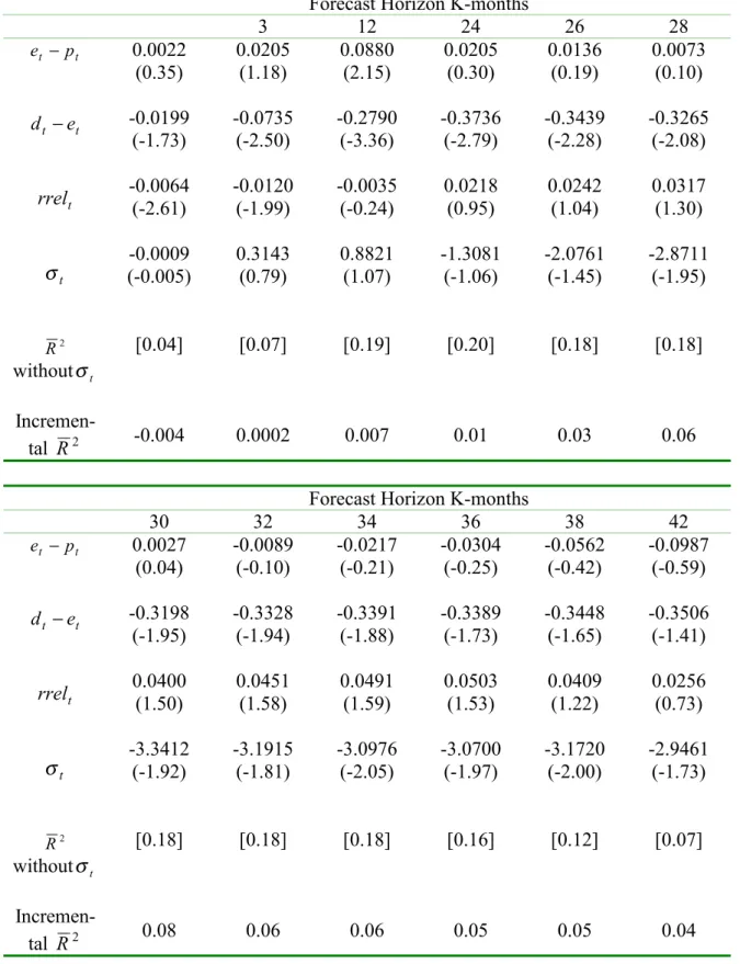
Table 4.Long-horizon Regression with Disperion and Other Forecasting variables Forecast Horizon K-months

1 3 12 24 26 28 t t p d − t t e d − t rrel t σ 2 R without_σt Incremen-tal _R2 0.0022 (0.35) -0.0221 (-1.73) -0.0064 (-2.61) -0.0009 (-0.005) [0.04] -0.004 0.0205 (1.18) -0.0940 (-2.65) -0.0120 (-1.99) 0.3143 (0.79) [0.07] 0.0002 0.0880 (2.15) -0.3670 (-3.69) -0.0035 (-0.24) 0.8821 (1.07) [0.19] 0.007 0.0205 (0.30) -0.3941 (-2.84) 0.0218 (0.95) -1.3081 (-1.06) [0.20] 0.01 0.0136 (0.19) -0.3576 (-2.50) 0.0242 (1.04) -2.0761 (-1.45) [0.18] 0.03 0.0073 (0.10) -0.3339 (-2.24) 0.0317 (1.30) -2.8711 (-1.95) [0.18] 0.06 Forecast Horizon K-months

30 32 34 36 38 42 t t p d − t t e d − t rrel t σ 2 R without_σt Incremen-tal _R2 0.0027 (0.04) -0.3226 (-2.02) 0.0400 (1.50) -3.3412 (-1.92) [0.18] 0.08 -0.0089 (-0.10) -0.3239 (-1.89) 0.0451 (1.58) -3.1915 (-1.81) [0.18] 0.06 -0.0217 (-0.21) -0.3174 (-1.78) 0.0491 (1.59) -3.0976 (-2.05) [0.18] 0.06 -0.0304 (-0.25) -0.3085 (-1.62) 0.0503 (1.53) -3.0700 (-1.97) [0.16] 0.05 -0.0562 (-0.42) -0.2886 (-1.51) 0.0409 (1.22) -3.1720 (-2.00) [0.12] 0.05 -0.0987 (-0.59) -0.2520 (-1.21) 0.0256 (0.73) -2.9461 (-1.73) [0.07] 0.04

Table 4 (continued)

The sample contains monthly observations from January 1982 to October 2000. The regression equation is r_t+1+L+r_t+K =a₀ +b₁(K)(d_t −p_t)+b₂(K)(d_t −e_t) K K t t t b K rrel K b₃( ) + ₄( ) + _{+ ,}

+ σ ε where r is monthly log real returns on the S&P 500

index, dt − pt is log dividend price ratio, dt −et is log dividend earnings ratio, rrelt is

the relative short-term Treasury bill rate (the three month Treasury bill rate minus its 12- month backward moving average), and _σt is the dispersion in forecasts. Numbers in parenthesis are Newey-West corrected t-statistics. R2 without _σt is the adjusted _R2

when _σt is excluded from the regression equation. Hence, only d_t − p_t, d_t −e_t, and

t

rrel are used as regressors. Incremental _R2 _{is the difference in R}2 _when

t

t p

d − ,

t

t e

d − , rrel_t, and _σt are used as regressors and when _σt is excluded from the regression.

Table 5. Long-horizon Regression with Disperion and Other Forecasting variables Forecast Horizon K-months

3 12 24 26 28 t t p e − t t e d − t rrel t σ 2 R withoutσ_t Incremen-tal R2 0.0022 (0.35) -0.0199 (-1.73) -0.0064 (-2.61) -0.0009 (-0.005) [0.04] -0.004 0.0205 (1.18) -0.0735 (-2.50) -0.0120 (-1.99) 0.3143 (0.79) [0.07] 0.0002 0.0880 (2.15) -0.2790 (-3.36) -0.0035 (-0.24) 0.8821 (1.07) [0.19] 0.007 0.0205 (0.30) -0.3736 (-2.79) 0.0218 (0.95) -1.3081 (-1.06) [0.20] 0.01 0.0136 (0.19) -0.3439 (-2.28) 0.0242 (1.04) -2.0761 (-1.45) [0.18] 0.03 0.0073 (0.10) -0.3265 (-2.08) 0.0317 (1.30) -2.8711 (-1.95) [0.18] 0.06 Forecast Horizon K-months

30 32 34 36 38 42 t t p e − t t e d − t rrel t σ 2 R withoutσ_t Incremen-tal R2 0.0027 (0.04) -0.3198 (-1.95) 0.0400 (1.50) -3.3412 (-1.92) [0.18] 0.08 -0.0089 (-0.10) -0.3328 (-1.94) 0.0451 (1.58) -3.1915 (-1.81) [0.18] 0.06 -0.0217 (-0.21) -0.3391 (-1.88) 0.0491 (1.59) -3.0976 (-2.05) [0.18] 0.06 -0.0304 (-0.25) -0.3389 (-1.73) 0.0503 (1.53) -3.0700 (-1.97) [0.16] 0.05 -0.0562 (-0.42) -0.3448 (-1.65) 0.0409 (1.22) -3.1720 (-2.00) [0.12] 0.05 -0.0987 (-0.59) -0.3506 (-1.41) 0.0256 (0.73) -2.9461 (-1.73) [0.07] 0.04

Table 5 (continued)

The sample contains monthly observations from January 1982 to October 2000. The regression equation is rt₊1+L+rt₊K =a0+b1(K)(et − pt)+b2(K)(dt −et) K K t t t b K rrel K b3( ) + 4( ) + ₊ ,

+ σ ε where r is monthly log real returns on the S&P 500

index, e_t − p_t is log earnings price ratio, d_t −e_t is log dividend earnings ratio, rrel_t is the relative short-term Treasury bill rate (the three month Treasury bill rate minus its 12-month backward moving average), and σ_t is the dispersion in earnings forecasts. Numbers in parenthesis are Newey-West corrected t-statistics. R2 without σt is the

adjusted _R2 _when

t

σ is excluded from the regression equation. Hence, only e_t − p_t,

t

t e

d − , and rrel_t are used as regressors. Incremental _R2 _{is the difference in R}2 _when

t

t p

e − , d_t −e_t, rrel_t, and _σt are used as regressors and when _σt is excluded from the regression.

Table 6. Long-horizon Regression with Dispersion and Macroeconomic Variables Forecast Horizon K-months

1 3 12 24 26 28 F (NW) 2 R withoutσt Incremen-tal R2 0.7078 0.0293 -0.0045 0.5811 0.0230 0.0015 0.0116 0.0591 -0.0089 5.4754 -0.0007 0.0693 7.7798 -0.0036 0.1108 8.6914 0.0063 0.1318 Forecast Horizon K-months

30 32 34 36 38 42 F (NW) 2 R without_σt Incremen-tal R2 8.3468 0.0102 0.1161 10.2566 0.0076 0.0937 6.7382 0.0115 0.0764 5.1119 0.0241 0.0710 4.2274 0.0251 0.0636 4.4460 0.0140 0.0507 The sample contains monthly observations from January 1982 to October 2000. The regression equation is r_t+1+L+r_t+k =a0 +γZ_t +b1σ_t +L+b_pσ_t−p +ε_t+k where r is monthly log real returns on the S&P 500 index, Z_t is a vector of current and lagged macroeconomic variables including the growth rate of industrial production, real short-term interest rate measured as the yield on three-month Treasury bill rate and CPI inflation rate, and σ_t is the dispersion in earnings forecasts. F (NW) is F-statistics corrected using Newey-West standard errors. R2 without σt is the R2 of the regression

when only macroeconomic variables are used as regressors. Incremental _R2 _{is the}

difference between R2 when macroeconomic variables and σt are used as regressors

Table 7. Market Volatility and Dispersion24

Regression Results Granger-Causality Test

Correlation

t

vol _R2 _{Volatility → Dispersion Dispersion → Volatility}

0.1680 0.3444

(2.64) 0.0239 2.6626 0.4455

2

R for regressions including Number of

lags

Lagged and Current Lagged, Current and future

1 0.0335 0.0402

3 0.0504 0.0568

6 0.0366 0.0422

12 0.0212 0.0242

The sample contains monthly observations from January 1982 to October 2000. Correlation shows the correlation between volatility and dispersion. Regression results show the results from the following regression σt =a0 +a1volt +εt where σt is the

dispersion and volt is the volatility. T-statistic in parenthesis is corrected using

Newey-West standard errors. Granger causality test shows the Wald test statistics under the null hypothesis that the volatility does not Granger-casue the dispersion (Volatility → Dispersion) or that the dispersion does not Granger-cause the volatility (Dispersion → Volatility). The lower panel of Table 7 shows the change in R2 when additional lagged volatility estimate is included in the regression. For future volatility, two led volatility estimates are used.

24 _{The volatility is estimated under GARCH (1,1) specification. However, volatility}

estimates under ARCH (1) and GARCH in Mean with AR (1) are almost identical to the volatility estimate under GARCH (1,1).

Table 8. Dispersion and Other Forecasting variables t t p d − dt −et rrelt R2 Coefficient -0.0098 0.0219 -0.0011 0.0588 t-statistics -2.16 3.75 -0.58 Incremental _R2 _{0.0512 0.0484 0.0006} Granger Causality (→σt) 2.2001 0.7462 0.3617 Granger Causality (σ →t ) 0.1239 1.0007 1.0160 t t p e − dt −et rrelt R2 Coefficient -0.0098 0.0122 -0.0011 0.0588 t-statistics -2.12 2.41 -0.56 Incremental R2 0.0512 0.0175 0.0006 Granger Causality (→σt) 4.4901 0.7462 0.3617 Granger Causality (_{σ →t} ) 0.2445 1.0007 1.0160 2

R for regressions including lagged and current

Number of lags d_t − p_t, d_t −e_t, rrel_t e_t −p_t, d_t −e_t, rrel_t

1 0.0992 0.0992

3 0.1732 0.1732

6 0.2134 0.2134

The sample contains monthly observations from January 1982 to October 2000. The regression equation is _σt =a0 +a1(d_t −p_t)+a2(d_t −e_t)+a3rrel_t +_εt or

t t t t t t t a a e p a d e a rrel ε

σ = 0 + 1( − )+ 2( − )+ 3 + . T-statistics are corrected using Newey-West standard errors. Incremental _R2 _{is the difference between R}2 _{when all these}

forecasting variables are included in the regression and _R2 _{when one of these variables}

is excluded in each case. Granger causality (→σt) is Wald statistics when bivariate

Granger causality test is conducted under the null hypothesis that a forecasting variable does not Granger-cause the dispersion. Granger causality (σ →t ) is Wald statistics when

bivariate Granger causality test is conducted under the null hypothesis that the dispersion does not Granger-cause a forecasting variable. The lowest panel of Table 8 shows the change in R2 when additional lagged forecasting variables are included in the regression.