Performance of combined double seasonal univariate time series models
for forecasting water demand
Jorge Caiadoa
aCenter for Applied Mathematics and Economics (CEMAPRE), Instituto Superior de Economia e Gestão, Technical University of Lisbon, Rua do Quelhas 6, 1200-781 Lisboa, Portugal. Tel.: +351 21 392 2715. E-mail: jcaiado@iseg.utl.pt
Abstract: In this article, we examine the daily water demand forecasting performance of double seasonal univariate time series models (Holt-Winters, ARIMA and GARCH) based on multi-step ahead forecast mean squared errors. A within-week seasonal cycle and a within-year seasonal cycle are accommodated in the various model speci…cations to capture both seasonalities. We investigate whether combining forecasts from di¤erent methods for di¤erent origins and horizons could improve forecast accuracy. The analysis is made with daily data for water consumption in Granada, Spain.
Keywords: ARIMA; Combined forecasts; Double seasonality; Exponential Smoothing; Forecasting; GARCH; Water demand.
1. Introduction
Water demand forecasting is of great economic and environmental importance. Many factors can in‡uence directly or indirectly water consump-tion. These include rainfall, temperature, demog-raphy, land use, pricing and regulation. Weather conditions have been widely used as inputs of multivariate statistical models for hydrological time series modelling and forecasting.
Maidment and Miaou (1986), Fildes, Randall and Stubbs (1997), Zhou, McMahou, Walton and Lewis (2000), Jain, Varshney and Joshi (2001) and Bougadis, Adamowski and Diduch (2005) adopted regression and time series models for wa-ter demand forecasting by using climate e¤ects as explanatory variables for their models. Wong, Ip, Zhang and Xia (2007) used a non-parametric ap-proach based on the transfer function model to forecast a time series of river‡ow. Jain and Ku-mar (2007) and Coulibary and Baldwin (2005) employed arti…cial neural networks methods for hydrological time series forecasting. Such meth-ods are useful for assessing water demand under some stability conditions. However, their ability to project demand into the future may be limited as a result of weather conditions variability and
changes in consumer behavior and technology. Water demand is highly dominated by daily, weekly and yearly seasonal cycles. The univari-ate time series models based on the historical data series can be quite useful for short-term demand forecasting as we accommodate the various pe-riodic and seasonal cycles in the model speci…-cations and forecasts. To avoid their sensibil-ity to changes in weather conditions and other seasonal patterns, we may combine forecasts de-rived from the most accurate forecasting methods for di¤erent forecast origins and horizons. Com-bining forecasts can reduce errors by averaging of individual forecasts (Clemen, 1989, Armstrong 2001) and is particularly useful when we are un-certain about which forecasting method is bet-ter for future prediction. Some relevant works on combined forecasts of univariate time series models are by Makridakis and Winkler (1983), Sanders and Ritzman (1989), Lobo (1992) and Makridakis, Chat…eld, Hibon, Lawrence, Mills, Ord and Simons (1993).
In this paper, we examine the water demand forecasting performance of double seasonal uni-variate time series models based on multi-step ahead forecast mean squared errors. We inves-tigate whether combining forecasts from di¤erent
methods and from di¤erent origins and horizons could improve forecast accuracy. Our interest in this problem arose from the time series competi-tion organized by Spanish IEEE Computacompeti-tional Intelligence Society at the SICO’2007 Conference. The remainder of the paper is organized as fol-lows. Section 2 describes the dataset used in the study. Section 3 discusses the methodology used in time series modelling and forecasting. Section 4 presents the empirical results. Section 5 o¤ers some concluding remarks.
2. Data
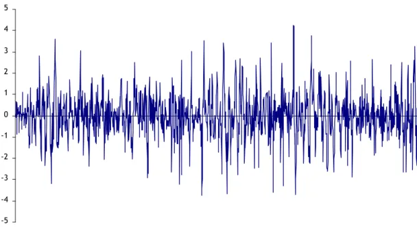
We analyze the daily water consumption se-ries in Spain from 1 January 2001 to 30 June 2006 (2006 observations). We have drop Febru-ary 29 in the leap year 2004 in order to main-tain 365 days in each year. This series is plotted in Figure 1. The dataset was obtained from the Spanish IEEE Computational Intelligence Society (http://www.congresocedi.es/2007/).
We use the …rst1976observations from 1 Jan-uary 2001 to 31 May 2006 as training sample for model estimation, and the remaining30 observa-tions from 1 June 2006 to 30 June 2006 as post-sample for forecast evaluation. The series exhibits periodic behavior with a within-week seasonal cy-cle of 7 periods and a within-year cycy-cle of 365 periods. The observed increases (decreases) in demand in the summer (winter) days seem to be caused by good (bad) weather. The analysis of weekly seasonality shows a consumption drop in demand on Saturdays and Sundays as a result of the shutdown of industry.
Figure 2 shows the sample autocorrelations (ACF) and the sample partial autocorrelations (PACF) for the training sample. The ACF de-cays very slowly at regular lags and at multiples of seasonal periods 7 and 365. The PACF has a large spike at lag 1 and cut o¤ to zero after lag 2. This suggests both a weekly seasonal dif-ference(1 B7)and a yearly seasonal di¤erence
(1 B365)to achieve stationarity. Figures 3 and 4 present the double seasonal di¤erenced series
(1 B7)(1 B365)Y
t and their estimated ACF
and PACF functions.
3. Methodology
3.1. Forecast evaluation
Denote the actual observation for time periodt
byYtand the forecasted value for the same period
by Ft. The mean squared error (MSE) statistic
for the post-sample periodt=m+1; m+2; :::; m+ his de…ned as follows: M SE = 1 h mX+h t=m+1 (Yt Ft)2. (1)
This statistic is used to evaluate the out-of-sample forecast accuracy using a training sam-ple of observations of size m < n(wherenis the sample size) to estimate the model, and then com-puting recursively the one-step ahead forecasts for time periods m+ 1, m+ 2, ... by increasing the training sample by one. For k-step ahead fore-casts, we begin at the start of the training sam-ple and we compute the forecast errors for time periods t=m+k, m+k+ 1, ... using the same recursive procedure.
3.2. Random walk
The naïve version of the random walk model is de…ned as
Ft+1=Yt. (2)
This purely deterministic method uses the most recent observation as a forecast, and is used as a basis for evaluating of time series models de-scribed below.
3.3. Exponential smoothing
Exponential smoothing is a simple but very useful technique of adaptive time series forecast-ing. Standard seasonal methods of exponen-tial smoothing includes the Holt-Winters’ addi-tive trend, multiplicaaddi-tive trend, damped addiaddi-tive trend and damped multiplicative trend (see Gard-ner, 2006). We implemented the double seasonal versions of the Holt-Winters’exponential smooth-ing (Taylor, 2003) in order to take into account the two seasonal cycle periods in the daily wa-ter consumption: a within-week cycle of 7 days and a within-year cycle of 365 days. In an ap-plication to half-hourly electricity demand, Tay-lor (2003) used a within-day seasonal cycle of 48
0 2 4 6 8 10 12 14
Jan-01 Jan-02 Jan-03 Jan-04 Jan-05 Jan-06
Figure 1. Daily water demand in Spain for the period 1 January 2001 to 30 June 2006
0 10 20 30 40 50 60 70 80 90 100 -0.5 0 0.5 1 ACF 0 10 20 30 40 50 60 70 80 90 100 -0.5 0 0.5 1 PACF
-5 -4 -3 -2 -1 0 1 2 3 4 5
Figure 3. Water demand series after yearly seasonal di¤erencing and weekly seasonal di¤erencing
0 10 20 30 40 50 60 70 80 90 100 -0.6 -0.4 -0.2 0 0.2 0.4 0.6 ACF 0 10 20 30 40 50 60 70 80 90 100 -0.6 -0.4 -0.2 0 0.2 0.4 0.6 PACF
half-hours and a within-week seasonal cycle of 336 half-hours.
The double seasonal additive methods outper-formed the double seasonal multiplicative ods. Within the double seasonal additive meth-ods, the additive trend was found to be the best for one-step ahead forecasting.
The forecasts for Taylor’s exponential smooth-ing for double seasonal additive method with ad-ditive trend are determined by the following ex-pressions: Lt= (Yt St 7 Dt 365) + (1 )(Lt 1+Tt 1) (3) Tt= (Lt Lt 1) + (1 )Tt 1 (4) St= (Yt Lt Dt 365) + (1 )St 7 (5) Dt= (Yt Lt St 7) + (1 )Dt 365 (6) Ft+h=Lt+Tt h+St+h 7+Dt+h 365+ h [Yt (Lt 1 Tt 1 St 7 Dt 365)] (7) whereLtis the smoothed level of the series;Ttis
the smoothed additive trend;Stis the smoothed
seasonal index for weekly period (s1 = 7); Dt
is the smoothed seasonal index for yearly period (s2 = 365); and are the smoothing para-meters for the level and trend; and are the seasonal smoothing parameters; is an adjust-ment for …rst-order autocorrelation; and Ft+h is
the forecast forhperiods ahead, withh 7. We initialize the values for the level, trend and sea-sonal periods as follows:
L365 = 1 365 365 X t=1 Yt T365 = 1 3652 730 X t=366 Yt 365 X t=1 Yt ! S1 = Y1 L7 ; S2= Y2 L7 ; :::; S7= Y7 L7 D1 = Y1 L365 ; D2= Y2 L365 ; :::; D365= Y365 L365 The smoothing parameters , , , and are chosen by minimizing the MSE statistic for one-step-ahead in-sample forecasting using a lin-ear optimization algorithm.
3.4. ARIMA model
We implemented a double seasonal multiplica-tive ARIMA model (see Box, Jenkins and Reinsel, 1994) of the form: p(B) P1(B s1) P2(B s2)(1 B)d (1 Bs1)D1(1 Bs2)D2(Y t c) = q(B) Q1(B s1) Q2(B s2)" t (8)
where c is a constant term; B is the lag opera-tor such that BkY
t=Yt k; p(B)and q(B)are
regular autoregressive and moving average poly-nomials of orders pand q; P1(B
s1), P2(B s2), Q1(B s1)and Q2(B
s2)are seasonal autoregres-sive and moving average polynomials of orders
P1, P2, Q1 and Q2; s1 and s2 are the seasonal periods; d, D1 and D2 are the orders of inte-gration; and "t is a white noise process with
zero mean and constant variance. The roots of the polynomials p(B) = 0, P1(B s1) = 0, P2(B s2) = 0, q(B) = 0, Q1(B s1) = 0 and Q2(B
s2) = 0 should lie outside the unit circle. This model is often denoted as ARIMA(p,d,q) (P1,D1,Q1)s1 (P2,D2,Q2)s2.
We examine the sample autocorrelations and the partial autocorrelations of the di¤erenced se-ries in order to identify the integer values p, q,
P1,Q1,P2 andQ2. After identifying a tentative ARIMA model, we estimate the parameters by Marquardt nonlinear least squares algorithm (for details, see Davison and MacKinnon, 1993). We check the adequacy of the model by using suit-able …tted residuals tests. We use the Schwarz Bayesian Criterion (SBC) for model selection. 3.5. GARCH model
In many practical applications to time series modelling and forecasting, the assumption of non-constant variance may be not reliable. The mod-els with nonconstant variance are referred to as conditional heteroscedasticity or volatility mod-els. To deal with the problem of heteroscedas-ticity in the errors, Engle (1982) and Boller-slev (1986) proposed the autoregressive condi-tional heteroskedasticity (ARCH) and the gener-alized ARCH (or GARCH) to model and fore-cast the conditional variance (or volatility). The
GARCH(p,q) model assumes the form: 2 t =!+ p X j=1 j 2t j+ q X i=1 i"2t i, (9)
where p is the order of the GARCH terms and
q is the order of the ARCH terms. The nec-essary conditions for the model (9) to be vari-ance and covarivari-ance stationary are: ! > 0;
j 0, j = 1; :::; p; i 0, j = 1; :::; q; and
Pp
j=1 j+
Pq
i=1 i <1. Last summation quan-ti…es the shock persistence to volatility. A higher persistence indicates that periods of high (slow) volatility in the process will last longer. In most economical and …nancial applications, the simple GARCH(1,1) model has been found to provide a good representation of a wide variety of volatil-ity processes as discussed in Bollerslev, Chou and Kroner (1992).
In order to capture seasonal and cyclical com-ponents in the volatility dynamics, we imple-mented a seasonal-periodic GARCH model of the form: 2 t = !+ 1 2t 1+ 1"2t 1+ 7"2t 7+ 365"2t 365 + M X k=1 kcos 2 kSt 7 +'ksin 2 kSt 7 +ukcos 2 kDt 365 +vksin 2 kDt 365 + 0k"2t 7cos 2 kSt 7 +'0k"2t 7sin 2 kSt 7 +u0k"2t 365cos 2 kDt 365 +vk0"2t 365sin 2 kDt 365 , (10)
whereStandDtare repeating step functions with
the days numerated from 1 to 7 within each week, and from 1 to 365 within each year, respectively. A similar approach was used by Campbell and Diebold (2005) to model conditional variance in daily average temperature data, and by Taylor (2006) to forecast electricity consumption. In the empirical study, we set M = 3 for the Fourier
series. We estimate the model by the method of maximum likelihood, assuming a generalized er-ror distribution (GED) for the innovations series (see Nelson, 1991).
3.6. Combining forecasts
We examine whether combining forecasts from the various univariate methods for di¤erent fore-cast origins and horizons could provide more ac-curate forecasts than the individual methods be-ing combined. The forecasts can be combined by using simple and optimal weights.
3.6.1. Simple combination
We consider all possible combinations of the forecast methods Holt-Winters (HW), ARIMA (A) and GARCH (G), and we compute the sim-ple (unweighted) average of the forecasts for one to seven days ahead,
FtS =F (HW) t +F (A) t +F (G) t 3 ; (11)
whereFt( )is the forecasted value of method( )in time periodt. This approach is simple and useful when we have no evidence about which forecast-ing method is more accurate. We drop the ran-dom walk (the worst method) of the combination. 3.6.2. Optimal combination
We consider two approaches for computing op-timal weights. Firstly, we compute the opop-timal combination of the forecasts using weights by the inverse of the MSE of each of the individual meth-ods (see Makridakis and Winkler, 1983), as fol-lows: FtM SE = h(M SE M SE(HW))Ft(HW) +(M SE M SE(A))Ft(A) +(M SE M SE(G))Ft(G)i 2M SE, (12) whereM SE=M SE(HW)+M SE(A)+M SE(G) is the sum of the post-sample forecast mean squared errors of the three methods.
Secondly, we compute optimal combination of the post-sample forecasts using weights by the in-verse of each of the forecast squared errors (SE)
of each of the individual methods, as follows: FtSE = h(SEt SEt(HW))F (HW) t +(SEt SEt(A))F (A) t +(SEt SEt(G))F (G) t i 2SEt, (13) where SEt = SEt(HW)+SE (A) t +SE (G) t is the
sum of the post-sample forecast squared errors of the three methods in time periodt.
4. Empirical study 4.1. Estimation results
The implementation of the double seasonal Holt-Winters method to the water demand se-ries Yt gives the values: = 0:000, = 0:755,
= 0:303, = 0:294 and = 0:607.
After evaluating di¤erent ARIMA formula-tions, we apply the following multiplicative dou-ble seasonal ARIMA model:
(1 1B 2B2 4B4)(1 1B7 2B14)
(1 B7)(1 B365)(Yt c)
= (1 9B9)(1 3B21)(1 1B365)"t
This model can be represented as ARIMA(4;0;9) (2;1;3)7 (0;1;1)365, with 3 = 0, 1 = = 8 = 0, and 1 = 2 = 0. The estimated results and diagnostic checks are shown in Table 1. All the parameter estimates are signi…cant at the 5% signi…cance level. The residual autocorrelation function (ACF) and par-tial autocorrelation function (PACF) exhibit no patterns up to order 7. The Ljung-Box statistic,
Q= 18:31, based on 20 residual autocorrelations is not signi…cant at the conventional levels. These results suggest that the model is appropriate for modeling the water demand series.
We then …tted a signi…cant parameter ARIMA-GARCH model of the form:
(1 1B 2B2 4B4)(1 1B7 2B14) (1 B7)(1 B365)(Yt c) = (1 9B9)(1 3B21)(1 1B365)"t and 2 t = !+ 1 2t 1+ 1"2t 1+ 365"2t 365 +'1sin 2 Dt 365 +' 0 3"2t 365sin 6 Dt 365 .
The model estimates and diagnostic checks are given in Table 2. The Ljung-Box test statistics show evidence of no serial correlation in the resid-uals (mean equation) and no serial correlation in the squared residuals (variance equation) up to order 20. Thus, we conclude that this model is also adequate for the data.
4.2. Forecast evaluation results
The performance of the estimated univariate methods were evaluated by computing MSE sta-tistics for multi-step forecasts from 1 to 7 days ahead.
Table 3 and Figure 5 give the forecasts results for the post-sample period from 1 June 2006 to 30 June 2006. An initial interpretation of the results suggests that the ability to forecast water demand did not decrease as the forecast horizon increased, except from 1 to 2 days ahead.
The ARIMA and GARCH models appear to have the same forecast performance especially for short-term forecasts (one to two days ahead). For one to four days ahead forecasts, the stochas-tic models ARIMA and GARCH performed bet-ter than the Holt-Winbet-ters method. In contrast, the Holt-Winters outperformed the ARIMA and GARCH models in long horizons. The random walk model ranked last for any of the forecast horizons considered.
The optimal combination of Holt-Winters, ARIMA and GARCH weighted by inverse squared errors is more accurate than the various simple combinations, except for 7-step ahead fore-casting in which the Holt-Winters outperformed the optimal combined forecasting. For one day ahead, the average MSE for the individual fore-casting methods (HW, ARIMA and GARCH) was 0.36 while it was 0.33 for the optimal com-bined forecasts –a error reduction of 8.33%. For two and three days ahead forecasts, combining reduced the MSE by 12.77% and 10.64%, respec-tively.
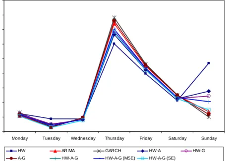
for each of the 7 days of the week in the same period. The results suggests that the Thursdays exhibit irregular demand patterns in the post-sample period used in this study. From the data, we found that the water consumption decreased 10.37% on the …rst Thursday of the post-sample period (1 June 2006), whereas it increased 4.22% and 18.44% on the following Thursdays (8 June 2006 and 15 June 2006, respectively). Possi-ble reasons for this unusual pattern are weather changes and any restrictions on water demand.
In terms of the day of the week e¤ect on fore-casting performance, the optimal combination HW-A-G (SE) appears to be most useful for Mon-day, Tuesday and Wednesday forecasts –combin-ing reduced the MSE of multi-step ahead aver-aged forecasts by 12.15%, 45.45% and 14.60%, re-spectively, when compared with the average of the individual methods. The Holt-Winters appears to be the most appropriate method for Thursday, Friday and Saturday forecasts and the GARCH model appears to be the best method for Sunday forecasts.
5. Conclusions
In this article we compared the forecast accu-racy of individual and combined univariate time series models for multi-step ahead daily water de-mand forecasting. We implemented double sea-sonal versions of the Holt-Winters, ARIMA and GARCH models in order to accommodate the two seasonal e¤ects (within-week cycle of 7 days and within-year cycle of 365 days) on the variability of the data.
The empirical results suggest that the optimal combined forecasts can be quite useful especially for short-term forecasting. However, the forecast-ing performance of this approach is not consis-tent over the seven days of the week. The deter-ministic method Holt-Winters and the stochastic method GARCH can be used independently to improve forecast accuracy on Thursdays to Sat-urdays and Sundays, respectively.
Acknowledgment: The author gratefully ac-knowledges the helpful comments of the partic-ipants in the Spanish IEEE Computational
In-telligence Society at the SICO’2007 Conference. This research was supported by a grant from the Fundação para a Ciência e a Tecnologia (FEDER/POCI 2010).
REFERENCES
1. Armstrong, J. (2001). "Combining forecasts",
in Principles of Forecasting: A Handbook for
Researchers and Practitioners, J. S.
Arm-strong (ed.), Kluwer Academic Publishers. 2. Bollerslev, T. (1986). "Generalized
au-toregressive conditional heteroskedasticity",
Journal of Econometrics, 31, 307-327.
3. Bollerslev, T., Chou, R. and Kroner, K. (1992). "ARCH modeling in Finance",
Jour-nal of Econometrics, 52, 5-59.
4. Bougadis, J., Adamowski, K. and Diduch, R. (2005). "Short-term municipal water dea-mand forecasting", Hydrological Processes, 19, 137-148.
5. Box, G., Jenkins, G. and Reinsel, G. (1994).
Time Series Analysis: Forecasting and Con-trol, 3rd ed., Prentice-Hall, New Jersey. 6. Campbell, S. and Diebold, F. (2005).
"Weather forecasting for weather deriva-tives", Journal of the American Statistical
Association, 100, 6-16.
7. Clemen, R. (1989). "Combining forecasts: a review and annoted bibliography",
Interna-tional Journal of Forecasting, 5, 559-584.
8. Coulibaly, P. and Baldwin, C. (2005): "Non-stationary hydrological time series forecasting using nonlinear dynamic methods", Journal
of Hydrology, 307, 164-174.
9. Davison, R. and MacKinnon, J. (1993).
Es-timation and Inference in Econometrics,
Ox-ford University Press, OxOx-ford.
10. Engle, R. (1982). "Autoregressive conditional heteroscedasticity with estimates of the vari-ance of United Kingdom in‡ation",
Econo-metrica, 50, 987-1008.
11. Fildes, R., Randall, A. and Stubbs, P. (1997). "One-day ahead demand forecasting in the utility industries: Two case studies",
Jour-nal of the OperatioJour-nal Research Society, 48,
15-24.
smooth-0,3 0,35 0,4 0,45 0,5 0,55
1-step 2-step 3-step 4-step 5-step 6-step 7-step
Forecast horizon (days)
MSE
HW ARIMA GARCH HW-A HW-G
A-G HW-A-G HW-A-G (MSE) HW-A-G (SE)
Figure 5. Comparison of multi-step ahead forecasts for post-sample period
0,00 0,50 1,00 1,50 2,00 2,50 3,00 3,50 4,00 4,50
Monday Tuesday Wednesday Thursday Friday Saturday Sunday
MSE
HW ARIMA GARCH HW-A HW-G
A-G HW-A-G HW-A-G (MSE) HW-A-G (SE)
ing: The state of the art - Part II",
Interna-tional Journal of Forecasting, 22, 637-666.
13. Jain, A., Varshney, A. and Joshi, U. (2001). "Short-term water demand forecast model-ing at IIT Kanpur usmodel-ing arti…cial neural net-works", Water Resources Management, 15, 299-231.
14. Jain, A. and Kumar, A.M. (2007). "Hybrid neural network models for hydrologic time se-ries forecasting", Applied Soft Computing, 7, 585-592.
15. Lobo, G. (1992). "Analysis and comparison of …nancial analysts, time series, and combin-ing forecasts of annual earncombin-ings", Journal of
Business Research, 24, 269-280.
16. Maidment, D. and Miaou, S. (1986). "Daily water use in nine cities",Water Resources
Re-search, 22, 845-851.
17. Madridakis, S. and Winkler, R. (1983). "Av-erage of forecasts: Some empirical results",
Management Science, 29, 987-996.
18. Madridakis, S., Chat…eld, C., Hibon, M., Lawrence, M., Mills, T., Ord. K. and Simons, L. (1993). "The M2-competition: A real-time judgmentally based forecasting study",
Inter-national Journal of Forecasting, 9, 5-22.
19. Nelson, D. (1991). "Conditional heteroskedas-ticity in asset returns: a new approach",
Econometrica, 59, 347-370.
20. Sanders, N. and Ritzman, L. (1989). "Some empirical …ndings on short-term forecast-ing: Technique complexity and combina-tions",Decision Sciences, 20, 635-640. 21. Taylor, J. (2003). "Short-term electricity
de-mand forecasting using double seasonal ex-ponential smoothing",Journal of the
Opera-tional Research Society, 54, 799-805.
22. Taylor, J. (2006). "Density forecasting for the e¢ cient balancing of the generation and con-sumption of electricity", International
Jour-nal of Forecasting, 22, 707-724.
23. Wong, H., Ip, W., Zhang, R. and Xia, J. (2007). "Non-parametric time series mod-els for hydrological forecasting", Journal of
Hidrology, 332, 337-347.
24. Zhou, S., McMahon, T., Walton, A. and Lewis, J. (2000). "Forecasting daily urban water demand: a case study of Melbourne",
Table 1
Seasonal ARIMA model estimates for water demand series
Model: ARIMA(4,0,9) (2,1,3)7 (0,1,1)365 Residual ACF Residual PACF Parameter Lag Estimate Standard error Lag Estimate Lag Estimate
c -0.004 0.007 1 0.004 1 0.004 1 1 0.592 0.025 2 0.009 2 0.009 2 2 0.134 0.027 3 -0.020 3 -0.020 4 4 0.061 0.023 4 0.001 4 0.001 9 9 -0.053 0.024 5 -0.026 5 -0.025 1 7 -0.757 0.023 6 0.015 6 0.015 2 14 -0.561 0.029 7 -0.010 7 -0.010 3 21 -0.366 0.032 1 365 -0.644 0.023 R2 adjusted = 0.662;Q(20) = 18:31(0.11).
Notes: Q(20) is the Ljung-Box statistic for serial correlation in the residuals up to order 20;p-value in parentheses.
Table 2
Seasonal-periodic GARCH model estimates for water demand series Model: ARIMA(4,0,9) (2,1,3)7 (0,1,1)365—GARCH(1,1) (0,1)365
Mean equation Residual ACF Residual PACF Parameter Lag Estimate Standard error Lag Estimate Lag Estimate
c -0.011 0.008 1 -0.007 1 0.007 1 1 0.502 0.029 2 0.023 2 0.023 2 2 0.137 0.030 3 -0.028 3 -0.028 4 4 0.075 0.024 4 -0.026 4 -0.026 9 9 -0.064 0.023 5 -0.042 5 -0.040 1 7 -0.747 0.023 6 0.026 6 0.027 2 14 -0.534 0.028 7 -0.006 7 -0.006 3 21 -0.346 0.031 1 365 -0.640 0.025
Variance equation Sq. residual ACF Sq. residual PACF Parameter Lag Estimate Standard error Lag Estimate Lag Estimate
! 0.107 0.028 1 0.012 1 0.012 1 1 0.103 0.037 2 -0.030 2 -0.031 1 1 0.483 0.108 3 0.028 3 0.029 365 365 0.109 0.032 4 0.018 4 0.016 '1 0.026 0.011 5 0.008 5 0.009 '0 3 365 0.062 0.035 6 -0.023 6 -0.023 GED 1.361 0.055 7 0.015 7 0.015 R2 adjusted = 0.657;Q(20)=19.20 (0.08);Q2(20)=13.61 (0.33).
Notes: Q(20) (Q2(20)) is the Ljung-Box statistic for serial correlation in the residuals (squared residuals) up to order 20;p-value in parentheses.
Table 3
MSE for multi-step-ahead forecasts for post-sample period
Forecast Simple combination Optimal combin.
horizon RW HW ARIMA GARCH HW-A HW-G A-G HW-A-G MSE SE 1-step 0.96 0.38 0.35 0.35 0.35 0.35 0.35 0.35 0.35 0.33 2-step 1.55 0.51 0.45 0.45 0.46 0.45 0.45 0.45 0.45 0.41 3-step 1.82 0.49 0.47 0.45 0.45 0.45 0.45 0.45 0.45 0.42 4-step 2.09 0.48 0.45 0.46 0.46 0.46 0.46 0.46 0.46 0.44 5-step 2.23 0.43 0.44 0.46 0.43 0.43 0.45 0.44 0.44 0.42 6-step 1.91 0.42 0.45 0.47 0.43 0.43 0.46 0.44 0.44 0.42 7-step 1.33 0.40 0.44 0.46 0.41 0.42 0.45 0.43 0.42 0.41 Average 1.70 0.44 0.44 0.44 0.43 0.43 0.44 0.43 0.43 0.41 Table 4
MSE for multi-step ahead forecasts for each day of the week in post-sample period
Forecast Day of the Simple combination Optimal combin.
horizon week RW HW ARIMA GARCH HW-A HW-G A-G HW-A-G MSE SE 1-step Monday 16.18 2.33 1.18 1.25 1.71 1.75 1.21 1.55 1.54 1.34 Tuesday 0.28 0.53 0.20 0.19 0.34 0.34 0.19 0.29 0.28 0.21 Wednesday 0.18 0.14 0.25 0.26 0.19 0.20 0.26 0.21 0.22 0.20 Thursday 3.15 4.19 5.26 5.40 4.71 4.78 5.33 4.93 4.94 4.84 Friday 0.47 0.37 0.54 0.54 0.45 0.45 0.54 0.48 0.48 0.35 Saturday 3.00 0.23 0.64 0.58 0.39 0.37 0.61 0.45 0.46 0.40 Sunday 1.20 1.26 0.40 0.33 0.70 0.61 0.36 0.53 0.53 0.41 4-step Monday 3.86 0.42 0.43 0.54 0.42 0.48 0.48 0.46 0.46 0.44 Tuesday 2.66 0.15 0.16 0.17 0.15 0.15 0.16 0.16 0.16 0.12 Wednesday 8.39 0.48 0.69 0.77 0.58 0.62 0.73 0.64 0.64 0.59 Thursday 11.27 3.63 3.79 4.14 3.71 3.88 3.96 3.85 3.85 3.73 Friday 1.83 1.78 1.88 1.94 1.83 1.86 1.91 1.87 1.87 1.84 Saturday 4.14 1.29 1.21 1.26 1.25 1.28 1.24 1.25 1.25 1.25 Sunday 10.23 3.23 1.10 0.81 2.03 1.82 0.95 1.56 1.55 1.18 7-step Monday 0.30 0.19 0.24 0.38 0.21 0.28 0.30 0.26 0.26 0.25 Tuesday 0.15 0.07 0.06 0.08 0.06 0.06 0.06 0.06 0.06 0.04 Wednesday 1.09 0.27 0.39 0.29 0.33 0.28 0.34 0.31 0.31 0.29 Thursday 13.60 2.54 3.33 3.42 2.92 2.96 3.38 3.08 3.07 2.99 Friday 7.91 2.14 2.25 2.38 2.19 2.26 2.32 2.26 2.25 2.17 Saturday 4.19 1.43 1.48 1.59 1.46 1.51 1.54 1.50 1.50 1.49 Sunday 0.70 1.14 0.29 0.22 0.63 0.51 0.26 0.42 0.44 0.31 Average Monday 4.79 0.61 0.55 0.65 0.57 0.62 0.59 0.59 0.59 0.53 Tuesday 4.13 0.44 0.16 0.17 0.25 0.26 0.16 0.21 0.21 0.14 Wednesday 4.89 0.43 0.46 0.48 0.41 0.41 0.47 0.42 0.42 0.39 Thursday 7.52 3.01 3.71 3.91 3.33 3.43 3.80 3.51 3.51 3.41 Friday 5.21 1.99 2.25 2.32 2.12 2.15 2.28 2.18 2.18 2.11 Saturday 4.02 1.06 1.24 1.26 1.13 1.14 1.25 1.17 1.17 1.13 Sunday 6.10 2.35 0.68 0.50 1.38 1.22 0.59 1.02 1.02 0.75