Business Analytics Using SAS Enterprise Guide and SAS Enterprise Miner A Beginner s Guide

(1)

Olivia Parr-Rud

Business Analytics Using

SAS

®

Enterprise Guide

®

and

SAS

®

Enterprise Miner

™

A Beginner’s Guide

(2)

Contents

About This Book ... vii

About the Author ... xi

Chapter 1: Defining the Business Objective ... 1

Introduction ... 1

Setting Goals ... 1

Descriptive Analyses ... 3

Customer Profile ... 3

Customer Loyalty ... 4

Market Penetration or Wallet Share ... 4

Predictive Analyses ... 4

Marketing Models ... 5

Risk and Approval Models ... 6

Predictive Modeling Opportunities by Industry ... 9

Notes from the Field ... 13

Chapter 2: Data Types, Categories, and Sources ... 15

Introduction ... 15

The Evolution of Data... 16

Types of Data ... 17

Nominal Data ... 17

Ordinal Data ... 17

Continuous Data ... 18

Categories of Data ... 18

Demographic or Firmographic Data ... 18

Behavioral Data ... 19

Psychographic Data ... 20 Full book available for purchase here.

(3)

Data Category Comparison ... 20

Sources of Data ... 21

Internal Sources ... 21

Storage of Data ... 27

External Sources ... 28

Chapter 3: Overview of Descriptive and Predictive Analyses ... 29

Introduction ... 29 Descriptive Analyses ... 30 Frequency Distributions ... 30 Cluster ... 33 Decision Tree ... 33 Predictive Analyses ... 35 Linear Regression ... 36 Logistic Regression ... 39 Neural Networks ... 41 Modeling Process ... 43

Define the Objective ... 43

Develop the Model ... 43

Implement the Model ... 48

Maintain the Model ... 49

Chapter 4: Data Construction for Analysis ... 53

Introduction ... 53

Data for Descriptive Analysis ... 53

Data for Predictive Analysis ... 54

Prospect Models ... 55

Customer Models ... 57

Risk Models ... 59

External Sources of Data ... 61

Chapter 5: Descriptive Analysis Using SAS Enterprise Guide ... 63

Introduction ... 63

(4)

Project Initiation ... 64

Exploratory Analysis ... 65

Importing the Data ... 65

Viewing the Data ... 66

Exploring the Data ... 66

Segmentation and Profile Analysis... 69

Correlation Analysis ... 76

Chapter 6: Market Analysis Using SAS Enterprise Guide ... 79

Introduction ... 79

Project Overview ... 79

Market Analysis ... 80

Project Initiation ... 80

Data Preparation ... 80

Penetration and Share of Wallet ... 89

Results ... 90

Chapter 7: Cluster Analysis Using SAS Enterprise Miner ... 93

Introduction ... 93

Cluster Analysis ... 94

Initiate the Project ... 94

Input the Data Source and Assign Variable Roles ... 97

Transform Variables ... 99

Filter Data ... 102

Build Clusters ... 104

Build Segment Profiles ... 107

Analyze Clusters and Recommend Marketing or Product Development Actions ... 109

Notes from the Field ... 109

Chapter 8: Tree Analysis Using SAS Enterprise Miner ... 111

Introduction ... 111

Decision Tree Analysis ... 112

(5)

Input the Data Source ... 114

Create Target Variable ... 115

Partition the Data ... 117

Build the Decision Tree ... 118

View the Decision Tree Output ... 120

Interpret the Findings ... 126

Alternate Uses for Tree Analysis ... 128

Notes from the Field ... 128

Chapter 9: Predictive Analysis Using SAS Enterprise Miner ... 129

Introduction ... 129

Select ... 130

Initiate the Project ... 130

Select the Data ... 131

Explore ... 133

StatExplore ... 133

MultiPlot ... 136

Modify ... 138

Replace Missing Values via Imputation ... 138

Partition Data into Subsamples ... 139

Manage Outliers ... 140

Transform the Variables ... 142

Model ... 145

Decision Tree ... 145

Neural Network ... 147

Regression ... 148

Assess ... 151

References ... 157

From Business Analytics Using SAS® Enterprise Guide® and SAS® Enterprise Miner™: A Beginner's Guide, by Olivia Parr-Rud. Copyright © 2014, SAS Institute Inc., Cary, North Carolina, USA. ALL RIGHTS RESERVED.

(6)

Chapter 6: Market Analysis Using SAS

Enterprise Guide

Introduction ... 79 Project Overview ... 79 Market Analysis ... 80 Project Initiation ... 80 Data Preparation ... 80

Penetration and Share of Wallet ... 89

Results ... 90

Introduction

Chapters 1 through 5 focused on general knowledge and techniques that laid the foundation for many types of data analysis. In this chapter, you will explore a more specific topic: competitive analysis.

When your company sets its strategy, the first questions to answer are as follows:

• What are the strengths and weaknesses of our primary competitors as compared to us? • What is our market share and how can we increase it?”

For most industries, data sources are available that allow companies to determine their market share, or “share of wallet,” within certain segments of the population. This analysis is valuable for setting marketing strategies, guiding research and development, and informing finance and budget allocations.

Project Overview

The leadership team at DMR Publishing Company is interested in understanding the drivers of revenue within its business. It has gathered U.S. customer data for the past year that consists of revenues, numbers of publications, and three demographic variables. For this analysis, you will use SAS Enterprise Guide.

(7)

The project has eight steps:

1.

Initiate the project in SAS Enterprise Guide 6.1.

2.

Import and view market data.

3.

Add the DMR Publishing customer SAS data set to the project.

4.

Use the query tool to build a new age group variable.

5.

Summarize the DMR Publishing customer data to a gender and age group level.

6.

Merge customer and market data.

7.

Summarize the merged data to age group level.

8.

Perform penetration and a “share of wallet” analysis.

Market Analysis

So far in this analysis, our main interest has been to describe the characteristics of the customer base. If possible, it can be useful to compare characteristics of the customer database with the same characteristics in the overall market. This comparison enables a penetration analysis and share of wallet analysis as defined in Chapter 1.

We have purchased a data set from General List Company that shows the annual revenues and number of subscriptions for the entire publishing market within the United States, segmented by gender and age group. Our goal is to compare performance within gender and age group between the DMR Publishing’s customer data and the total market data purchased from General List Company.

Project Initiation

Similar to the process in Chapter 5, the first step is to open the project. Double click the SAS Enterprise Guide icon. Select New Project.

Data Preparation

Your first step is to prepare the data.

Import Data

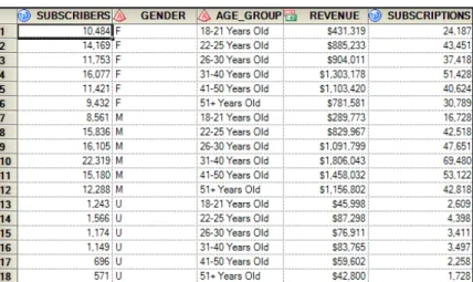
To access the data, go to File  Import and choose the Publishing Market data set. When the first window opens, click Finish. Notice that the data is already summarized as shown in Output 6.1.

(8)

Output 6.1: Publishing Market Data

To create the penetration and wallet analyses, merge the market data to the DMR Publishing customer data. Before you can merge the two data sets, you need to summarize the customer data. We plan to merge the two data sets by gender and age group.

The GENDER field is ready to match, but you must create the AGE_GROUP variable in the DMR Publishing customer data.

Because we started a new project, we need to bring the DMR Publishing customer data into the project. In the top menu, select View Server List. A new window will open below the Project Tree window; it will display the servers, as shown in Figure 6.1.

(9)

Click the plus sign to the left of Servers. Continue to expand until you reach the SASUSER library as shown in Figure 6.2.

Figure 6.2: Expand Library to Locate DMR Publishing Customer Data

Right-click the DMR_CUSTOMER_BASE data and select Open. The data has now been added to the project and is visible in the Project Tree. You are ready to create the Age Group variable in the DMR Publishing customer data.

Build Age Group Variable

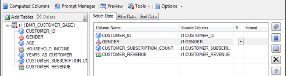
Right-click the DMR Customer data set and select Query Builder as shown in Figure 6.3. Drag four variables from the left over to the right column: GENDER, CUSTOMER_ID,

CUSTOMER_SUBSCRIPTION_COUNT, and CUSTOMER_REVENUE. Figure 6.3: Query to Build Age Group on DMR Publishing Customer Data

(10)

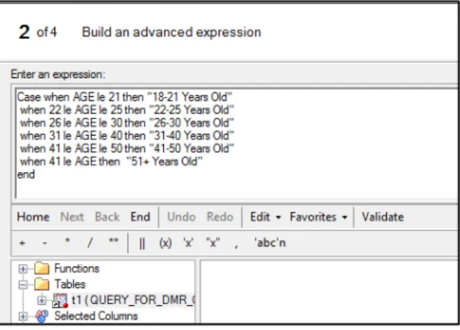
Next, click Computed Columns  New  Advanced Expression  Next (Figure 6.4). Figure 6.4: Expression Builder to Create Age Group Variable

The window has a space to enter an expression. Program 6.1 displays the syntax for building the variable in the Query Builder; copy it into the box under Enter an expression.

Program 6.1: Expression Builder to Create Age Group Variable Case when AGE le 21 then "18-21 Years Old" when 22 le AGE le 25 then "22-25 Years Old" when 26 le AGE le 30 then "26-30 Years Old" when 31 le AGE le 40 then "31-40 Years Old" when 41 le AGE le 50 then "41-50 Years Old" when 51 le AGE then "51+ Years Old"

end

Click Next. In the next window’s field, type AGE_GROUP in the top box next to Column Name. Click Finish  Close.

(11)

Sum Performance Variables

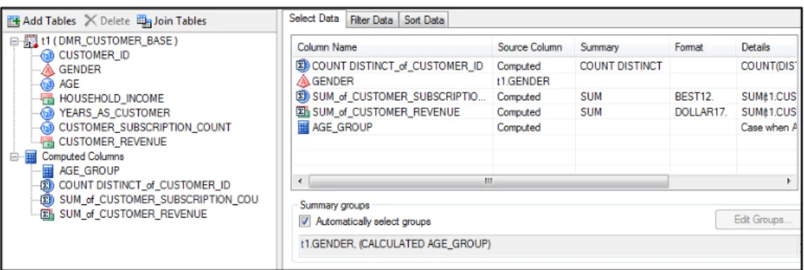
The next step is to sum the performance variables CUSTOMER_ID, CUSTOMER_REVENUE, and CUSTOMER_SUBSCRIPTION_COUNT (Figure 6.5). Within the same query, on the right-hand side, put your cursor next to CUSTOMER_ID under the Summary column. An arrow will appear. Scroll down and select COUNT DISTINCT. For easier viewing, you can adjust the column widths with your cursor. Next, right-click the space next to CUSTOMER_REVENUE and

CUSTOMER_SUBSCRIPTION_COUNT and select SUM. You’ll notice that a Summary groups

pane appears at the bottom right section of the window. The software guesses GENDER and CALCULATED AGE_GROUP, which is correct. Click Run.

Figure 6.5: Sum Performance Variables across Gender and Age Group

In Output 6.2, the data set appears to be summarized correctly. The new summary variables have the prefix SUM_. We will use these variables in the penetration and wallet analyses.

(12)

Merge Customer and Market Data

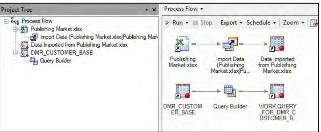
The next step is to merge the data. If you don’t see the Process Flow on the right side of your screen, double-click on Process Flow in the top left corner at the top of the Project Tree, and it will appear in the work area on the right as seen in Figure 6.6.

Figure 6.6: Select Data for Merge Query

Right-click the newly summarized data and select Query Builder. After the window opens, drag all the variables from t1 (QUERY_FOR_DMR_CUSTOMER_BASE) into the right-hand column. In the upper left-hand corner, look for Join tables. A new window will open with the fields in the new data set. Click Add Tables. Select WORK.PUBLISHING_MARKET (Figure 6.7). If you can’t see the whole name, put your cursor over the fields. The full name will appear. Click Open. Figure 6.7: Select Data for Join

The software will guess a match variable. In this case, it guesses GENDER. But, it is an inner join as shown in the Venn diagram. Right-click on the circles and select Properties. You want to match the records in the DMR Publishing customer data that finds a match in the Publishing Market data; therefore, from the list at the top, select All rows from the right table given the condition ( Right Join ). Also, notice just below the circles that it asks if you want t2.GENDER to equal (=)

(13)

You are also going to match on AGE_GROUP. Right-click on AGE_GROUP in the first data set (t1). Follow the prompt to match to AGE_GROUP in the second data set (t2). Next, a window will appear, and a prompt will ask you what kind of join you want to select (Figure 6.8). As directed in the first join using GENDER, you want to match the records in the DMR Publishing customer data that finds a match in the Publishing Market data; therefore, select All rows from the right table given the condition (Right Join ). Also, notice just below the circles that asks if you want t2.AGE_GROUP to equal (=) t1.AGE. The default is correct. Click Close.

Figure 6.8: Merge of DMR Customer and Market Data Sets

You will be back in the main screen of the query builder. From the left column, drag the following variables from the (t2) PUBLISHING_MARKET to the right side under Column Name:

SUBSCRIBERS, REVENUE, SUBSCRIPTIONS (Figure 6.9). Figure 6.9: Add Variables from Publishing Market Data

(14)

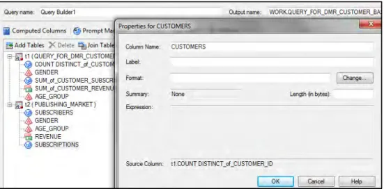
Figure 6.10: Rename Three Columns to Business-Related Names

Double-click under Column Name on the right, where COUNT DISTINCT appears. When the window opens, type in a new name, such as CUSTOMERS. Click OK. Repeat the process for the two other summary columns. Suggested names are CUSTOMER_SUBS and

CUSTOMER_REVENUE. Now, click Run.

The merged data shows a perfect match between the customer data and the market data. Notice that it is at the GENDER-by-AGE_GROUP level.

Output 6.3: Merged Data at Gender and Age Group Level

For your current analysis, you want to look atpenetration and share of wallet by age group. So, you will summarize the data one more time. Return to the Process Flow and right-click the merged data and select Query Builder.

(15)

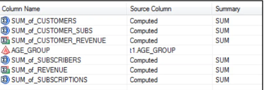
When the window opens, drag each variable except GENDER to the right side and drop it under

Column Name. Put your cursor in the empty space under Summary, and a dropdown menu will appear with the word NONE (Figure 6.11). Click and select SUM next to each variable except AGE_GROUP.

Figure 6.11: Summing of Merged Data to Age Group Level

When you are finished, click Run. This step summarizes all the customer and market values to the AGE_GROUP level. Review and close the data view.

Calculate the Share of Wallet

The next step is to calculate the share of wallet for customers, subscriptions, and revenues with use of the query tool. With your cursor on the summarized data, right-click and then click Query Builder. Once it opens, pull all of the variables into the right-hand pane. You can pull each variable separately or move the entire data set at one time by dragging the icon where t1 (QUERY_FOR_DMR appears). For ease of viewing, widen the Column Name heading on the right side until you can see the full column names.

Next, go to Computed ColumnsNewAdvanced ExpressionNext. In the box under

Advanced Expression, type SUM_of_CUSTOMERS/SUM_of_SUBSCRIBERS and click Next (Figure 6.12). Type PCT_of_SUBSCRIBERS next to Column Name. At the bottom of the window, next to Format, click Change and select Numeric and Percentw.d. Leave other settings unchanged as default. Click OKFinish. In the remaining window, click Close.

(16)

Figure 6.12: Computed Columns to Create Percentage Variables

Next, click New and type SUM_of_CUSTOMER_SUBS/SUM_of_SUBSCRIPTIONS. Click Next

and name the fraction PCT_of_SUBSCRIPTIONS. Create the same format and click Finish. Repeat the process with SUM_of_CUSTOMER_REVENUE/SUM_of_REVENUE in the box. Use the same format. Click Next and name the fraction PCT_of_REVENUE. Click Next  Finish. Click Close  Run.

NOTE: To avoid errors, variable names must be exactly as stated. Output 6.4 displays the final percentage values.

Output 6.4: Final Percentage Variables Showing Percent of DMR Subscriber Measures as Percent of Total Market

Penetration and Share of Wallet

Your data is now ready to analyze. To get a clear view by AGE_GROUP, close the data and highlight the last created data set. Click Tasks  Describe  List Data. This process allows you to take the variables or columns that you select and print them in a report format. The window in Figure 6.13 allows you to manage the report output.

(17)

Figure 6.13: Creation of a Report

Drag AGE_GROUP and the three percentage (PCT) variables to the right side. Click Run. Look for the output created in Microsoft Word.

Results

Reporting your results is one of the most important steps in your analysis. If you do everything right and can’t communicate the results, your efforts and insights will be wasted.

In Output 6.5, the final report displays the market penetration analysis and share of wallet by age group. When you are evaluating the percentage of subscribers, the lowest market penetration is in the 18 to 21-year-old age group. It is higher with 26 to 50-year-olds, at 10% to 11%. It drops slightly at age 51 or older (9%).

(18)

The percentage of subscriptions shows a different outcome. The youth, aged 18 to 21 years, have a higher number of subscriptions per person. So, they bring in the largest percentage of the revenue. Their share of wallet is 14%, compared with only 6% for those aged 51 or older.

Several conclusions can be drawn from this analysis. If you are looking for additional subscribers that bring in high average revenue, the 18- to 21-year-old market is the place to focus. These subscribers seem to be happiest with the current offerings, although there is still much room to grow.

On the other hand, growth opportunities for the business may emerge in the other age groups if new products are emphasized. The share of wallet is 10% or less for customers aged 22 years or older. This result suggests that products could be developed to appeal to groups older than 21.

Notes from the Field

This case study provides some rich insights and potential opportunities for DMR Publishing. What the company does with the information depends much more on the abilities of the organization. Consider that there are two new opportunities identified. The first opportunity is to find additional subscribers that look like their current subscriber base. The job of finding additional subscribers might be handled by the marketing department. The second opportunity is to create new products for the underserved areas of the market. This need for new products would likely be a project for the product development side of the business. The optimal solution may be a mixture of both departments.

Because both market growth for the current business and product development are important, management must make the decision about how to allocate resources. The best outcomes are seen when companies have fostered a culture of big data so that departments are able to collaborate and partner in the implementation of the analysis results, optimizing profits for the overall company.

FromBusiness Analytics Using SAS®_Enterprise

Guide®_{and SAS}®_{Enterprise Miner}_™_. Full book available for purchase here.

(19)

A

Account Number

in B2C customer database 22 in transaction database 24 activation model 5

Activity Amount, in transaction database 24 Activity Date, in transaction database 24 Activity Type, in transaction database 24 Actual Performance, in model log 50 Advanced Expression function 70 Age Group variable 82–83

airline industry, predictive modeling opportunities for 12 analysis

See also data

See also descriptive analysis See also predictive analysis categorical data 68 correlation 76–77 interval data 68 linear regression 36–39 market penetration 4 profile 69–76 Apache Hadoop 26–27 approval models 6–9

art schools, predictive modeling opportunities for 11

Assess step, in model development 130, 151– 155

attitudinal data 20 attrition 6, 59

See also retention/loyalty/attrition model auto industry, predictive modeling opportunities

for 12

auto insurance companies, predictive modeling opportunities for 10

average performance 45

B

B2B (business to business) customer database 22–23

B2C (business to consumer) customer database 21–22

banks, predictive modeling opportunities for 9– 10

behavioral data 19

"Big Data: What It Is and Why It Matters" 16– 17

binary variables 70, 71

biotech industry, predictive modeling opportunities for 12 business objective about 1 descriptive analysis 3–4 predictive analyses 4–12 setting goals 1–3

business to business (B2B) customer database 22–23

business to consumer (B2C) customer database 21–22

C

C statistic 47–48

cable companies, predictive modeling opportunities for 10

casinos, predictive modeling opportunities for 11

casualty insurance companies, predictive modeling opportunities for 10 catalog companies

predictive modeling opportunities for 10 for retailers 10

categorical data analysis 68 categorical variables 17, 74–76 cellular companies, predictive modeling

(20)

chemical industry, predictive modeling opportunities for 12 churn 6, 59 claims 7 class variables 17, 30–31 classification tree 34

cluster analysis (clustering) 33

See also SAS Enterprise Miner, cluster analysis using Cluster icon 104 clusters analyzing 109 building 104–106 Cody, Ron

Cody's Data Cleaning Techniques Using SAS 66

Cody's Data Cleaning Techniques Using SAS (Cody) 66

collection model, for banks 10

colleges, predictive modeling opportunities for 11

columns, renaming 86–87

community, predictive modeling opportunities for 12 Company ID in B2B customer database 23 in contact database 24 Company Name in B2B customer database 23 in contact database 24

Company URL, in B2B customer database 23 complexity, of data 17

computer hardware/software, predictive modeling opportunities for 11 contact database 23–24

Contact ID

in contact database 23 in score database 25 in transaction database 24 Contact Name, in contact database 23 continuous data 18, 68

continuous data analysis 68

continuous variables 31–32, 72–73, 76–77

correlation analysis 76–77 Count, in nodes 124

Create Data Source icon 131 Create icon 101, 115

credit card banks, predictive modeling opportunities for 9–10 cross-sell/up-sell model

about 5 for banks 10 cases 57

for gaming industry 11

for hospitality and travel industry 12 for insurance companies 10

for retailers 10

for technology companies 11

for telecommunications companies 10 using life-stage segments 58–59 for utility companies 11

CR_TOP_25PCT build expression 71–72 cumulative lift 46

customer data, merging with market data 85–88 Customer ID

in B2C customer database 21–22 in marketing database 25 in score database 25 in transaction database 24 customer life cycle 8–9 customer models 57–59

Customer Name, in B2C customer database 22 customers

fraud risk for 60 insurance risk for 60–61 leveraging your best 126 loyalty of 4

profile for 3–4

targeting your worst 126

D

data

about 15, 53 attitudinal 20 behavioral 19

(21)

categories of 18–21 continuous 18, 68 customer 85–88 demographic 18–19

for descriptive analysis 53–54 evolution of 16–17 exploring 66–69 external sources of 27, 61 filtering 102–104 firmographic 18–19, 23 importing 65, 80–82 internal sources of 21–25 lifestyle 20 market 85–88 nominal 17 ordinal 17 partitioning 117–118, 139–140 partitioning into subsamples 139–140 for predictive analysis 54–61

psychographic 20 ratio 18 selecting 131–133 sources of 21–27 storage of 26–27 types of 17–18 viewing 66

data category comparison 20–21 Data Partition icon 117, 118 data source 97–99, 114–115 Data Sources icon 97 data warehouse 26

Date, in marketing database 25 decision tree 145–147

decision tree analysis 33–35, 120–126, 128 See also SAS Enterprise Miner, tree analysis

using

Decision Tree icon 118, 145

Decision Trees for Analytics Using SAS Enterprise Miner (DeVille and Neville) 44

default models about 7 for banks 9

for insurance companies 10

for telecommunications companies 10 for utility companies 11

default risk, for prospects 60 Delwiche, Lora D.

The Little SAS Book for Enterprise Guide 65

demographic data 18–19

Demographic Information, in B2C customer database 22

dependent variables 132 descriptive analysis

about 29, 30

cluster analysis (clustering) 33 customer loyalty 4

customer profile 3–4 data for 53–54

decision tree analysis 33–35 external sources of data 61 frequency distributions 30–32 modeling process 43–51

using SAS Enterprise Guide. See SAS

Enterprise Guide, descriptive analysis using

DeVille, Barry

Decision Trees for Analytics Using SAS Enterprise Miner 44

diagnostics, of decision trees 123–124 discrete variables 17

distribution analysis, selecting variables for 70 DMR_CUSTOMER_DATA icon 115

DUNS Number, in B2B customer database 23

E

education, predictive modeling opportunities for 11, 12

electric companies, predictive modeling opportunities for 11–12 Email Address

in B2C customer database 22 in contact database 24

(22)

entertainment industry, predictive modeling opportunities for 10–11

Expected Loss Given Default, in score database 25

Expected Performance, in model log 50 Expected Value, in score database 25

Explore step, in model development 130, 133– 138

Expression Builder, creating Age Group variables with 83

external sources, of data 27, 61

F

failure model

for entertainment and social media industry 11

for utility companies 12 Filter icon 103–104, 140, 141, 142 filtering data 102–104

firmographic data 18–19, 23

food industry, predictive modeling opportunities for 12

former/lapsed customer, of customer life cycle 8–9

fraud 7–8 fraud model

for banks 10

for gaming industry 11 for insurance companies 10 for Public sector and nonprofit 12 for telecommunications companies 10 for utility companies 12

fraud risk, for customers 60 frequency distributions 30–32

G

gains chart 46–47 gains table 45–46

gaming industry, predictive modeling opportunities for 11

gas companies, predictive modeling opportunities for 11–12

geo usage model, for transportation and shipping industry 12

goal setting 1–3

government, predictive modeling opportunities for 12

graph properties, of decision trees 121–122

H

Hadoop 26–27

Headquarter ID, in B2B customer database 23 health insurance companies, predictive modeling

opportunities for 10

healthcare industry, predictive modeling opportunities for 12

hospitality and travel industry, predictive modeling opportunities for 12 hotels, predictive modeling opportunities for 12 Household ID, in B2C customer database 22

I

importing data 65, 80–82

imputation, replacing missing values via 138– 139

Impute function 145 Impute icon 138, 139 indicator variables 17

industry, predictive modeling opportunities by 9–12

inputting data source 97–99, 114–115 insurance companies, predictive modeling

opportunities for 10 insurance risk, for customers 60–61

Interactive setting (decision tree analysis) 119 internal sources, of data 21–25

Internet companies, predictive modeling opportunities for 10

(23)

K

Key Drivers, in model log 50

L

life insurance companies, predictive modeling opportunities for 10

life-stage segments, up-sell model using 58–59 lifestyle data 20

lifetime value (LTV) 8–9 lift 46

line width, of nodes 124 linear function 39

linear regression analysis 36–39 link function 41

The Little SAS Book for Enterprise Guide (Delwiche and Slaughter) 65 logistic regression 39–41

logit function 40

loss-given-default models 7, 60 loyalty

See also retention/loyalty/attrition model about 6

cases 59 customer 4

LTV (lifetime value) 8–9

M

manufacturing industry, predictive modeling opportunities for 12

market analysis

See SAS Enterprise Guide, market analysis

using

market data, merging with customer data 85–88 market penetration analysis 4

marketing database 25 marketing models 5–6

Maximum Branch setting (decision tree analysis) 119

Maximum Depth setting (decision tree analysis) 119

Merge Query, selecting data for 85

merging customer and market data 85–88 metadata, attaching to transform variables 116–

117

Metadata icon 116, 117, 118 Microsoft Word icon 68

missing values, replacing via imputation 138– 139

Model Comparison icon 151 Model Comparison node 151–155 Model Details, in model log 50 Model Developer, in model log 50

Model Development Campaign Data, in model log 50

Model Implementation Campaign Data, in model log 50

Model Implementation Launch Date, in model log 50

model log 50–51

Model Name, in model log 50 model of life 49

Model Scores

in B2B customer database 23 in B2C customer database 22 in contact database 24

Model step, in model development 130, 145– 150

Model Type, in model log 50 modeling data set 54

modeling process 43–51 models

See also specific models

developing in modeling process 43–48 implementing in modeling process 48 maintaining in modeling process 49–51 Modify step, in model development 130, 138–

144

mortgage banks, predictive modeling opportunities for 9–10 multicollinearity 45

multiple linear regression 38–39 MultiPlot icon 136

(24)

N

Neural Network icon 147 neural networks 41–42, 147–148 Neville, Padraic

Decision Trees for Analytics Using SAS Enterprise Miner 44

new/established customer, of customer life cycle 8–9

node characteristics, of decision trees 124 Node ID 124

node interpretation, of decision trees 125–126 nominal data 17

O

objectives, defining in modeling process 43 Offer Detail, in marketing database 25 offline retailers 10

online gaming, predictive modeling opportunities for 11 online retailers 10

online sharing sites, predictive modeling opportunities for 10–11 ordinal data 17

outliers, managing 140–142 Overall Objective, in model log 50

P

Partition icon 139 partitioning

data 117–118, 139–140 data into subsamples 139–140 penetration, share of wallet and 89–90 Percentage, in nodes 124

performance variables 84 performance window 54

pharmaceutical industry, predictive modeling opportunities for 12 Phone Number in B2B customer database 23 in B2C customer database 22 in contact database 24 Physical Address in B2B customer database 23 in B2C customer database 22 in contact database 24

politics, predictive modeling opportunities for 12

predictive analysis

See also SAS Enterprise Miner, predictive analysis using

about 29, 35–36, 54–55 customer models 57–59 data for 54–61

linear regression analysis 36–39 logistic regression 39–41 marketing models 5–6 modeling process 43–51 neural networks 41–42 prospect models 55–57 risk models 59–61 Pre-Selects, in model log 50

Probability to Buy, in score database 25 Probability to Default, in score database 25 process failure model

for hospitality and travel industry 12 for manufacturing industry 12 for technology companies 11

for telecommunications companies 10 for transportation and shipping industry 12 product failure model, for manufacturing

industry 12

Product or Service ID, in B2B customer database 23

Products or Services, in B2C customer database 22

profile analysis 69–76 profiling

selecting categorical variables for 74–76 selecting continuous variables for 72–73 property insurance companies, predictive

modeling opportunities for 10 Property menu (Add-Cluster process) 104, 105 Prospect ID, in marketing database 25

(25)

prospect phase, of customer life cycle 8–9 prospects

buying more 126 default risk for 60

loss-given-default risk for 60 psychographic data 20

public sector and nonprofit industry, predictive modeling opportunities for 12

Q

Query Builder

building Age Group variables with 82–83 creating binary variables with 70, 71

R

radio industry, predictive modeling opportunities for 10–11

rail industry, predictive modeling opportunities for 12

ratio data 18 rebuild 49

recruitment model, for sports industry 12 refresh 49

regression 148–150 Regression icon 148

religion, predictive modeling opportunities for 12

resorts, predictive modeling opportunities for 12 response models

about 5 for banks 9 for education 11

for manufacturing industry 12 for Public sector and nonprofit 12 for retailers 10

restaurants, predictive modeling opportunities for 12

retail banks, predictive modeling opportunities for 9–10

retail companies, predictive modeling opportunities for 10

retailers, predictive modeling opportunities for 10

retention model, for education 11 retention/loyalty/attrition model

for banks 10

for retailers 10

revenue models about 5 for banks 10

for hospitality and travel industry 12 for manufacturing industry 12 for Public sector and nonprofit 12 for retailers 10

for telecommunications companies 10 risk models 6–9, 59–61

S

SAS Enterprise Guide, descriptive analysis using about 63

correlation analysis 76–77 exploratory analysis 65–69 project initiation 64–65 project overview 63–64

(26)

segmentation and profile analysis 69–76 Task menu 67

SAS Enterprise Guide, market analysis using about 79

building Age Group variable 82–83 calculating share of wallet 88–89 data preparation 80–89

importing data 80–82 market analysis 80–89

merging customer and market data 85–88 penetration and share of wallet 89–90 project initiation 80

project overview 79–80 results 90–91

summing performance variables 84 SAS Enterprise Guide icon 64, 80

SAS Enterprise Miner, cluster analysis using about 93

analyzing clusters 109 assigning variable roles 97–99 building clusters 104–106

building segment profiles 107–108 cluster analysis 94–109

filtering data 102–104 initiating the project 94–96 inputting data source 97–99 project overview 93–94 transforming variables 99–102

SAS Enterprise Miner, predictive analysis using about 129–130

Assess step 151–155 decision tree 145–147 Explore step 133–138 initiating the project 130–131 managing outliers 140–142 Model step 145–150 Modify step 138–144 MultiPlot node 136–138 neural network 147–148

partitioning data into subsamples 139–140 regression 148–150

replacing missing values via imputation 138–139

Select step 130–133 selecting data 131–133 StatExplore node 133–136 transforming variables 142–144 SAS Enterprise Miner, tree analysis using

about 111

building decision tree 118–119 creating target variables 115–117 decision tree analysis 112–128 initiating the project 112–114 inputting data source 114–115 interpreting findings 126–128 partitioning data 117–118 project overview 111–112

viewing decision tree output 120–126 SAS Enterprise Miner icon 94

savings and loan banks, predictive modeling opportunities for 9–10

score database 24–25

Score Distribution, in model log 50 Segment Plot 105–106

Segment Profile icon 107

segment profiles, building 107–108 Segment Size 105–106

segmentation 69–76

Select step, in model development 130–133 Selection Business Logic, in model log 50 Selection Criteria, in model log 50 selection method 44

shading, of nodes 124 share of wallet

calculating 88–89 penetration and 89–90

shipping industry, predictive modeling opportunities for 12 sigmoidal function 40, 42 Slaughter, Susan J.

The Little SAS Book for Enterprise Guide 65

social media activity, as form of behavioral data 19

(27)

social media industry, predictive modeling opportunities for 10–11 social network data 19

Specific Target, in model log 50 sports industry, predictive modeling

opportunities for 12 StatExplore icon 133

StatExplore node 133–136 storage, of data 26–27

summing performance variables 84

T

Table icon 152 target model

for Public sector and nonprofit 12 for sports industry 12

target variables 115–117

Task menu (SAS Enterprise Guide) 67 technical colleges, predictive modeling

opportunities for 11

technology companies, predictive modeling opportunities for 11

telecommunications companies, predictive modeling opportunities for 10 television industry, predictive modeling

opportunities for 10–11

Time of Model Development, in model log 50 transaction database 24

Transform function 98

Transform Variables icon 99, 102, 115, 116, 142, 143

transforming variables 99–102, 142–144 transportation and shipping industry, predictive

modeling opportunities for 12 tree analysis

See SAS Enterprise Miner, tree analysis

using trends 19

trucking industry, predictive modeling opportunities for 12

U

unique identifier 27

universities, predictive modeling opportunities for 11

up-sell model

See cross-sell/up-sell model

usage model about 5

for hospitality and travel industry 12 for manufacturing industry 12 for Public sector and nonprofit 12

for transportation and shipping industry 12 for utility companies 11

utility companies, predictive modeling opportunities for 11–12

V

values, of nodes 124 variability, of data 16–17 variables adding 86, 86f Age Group 82–83

assigning roles for 97–99, 114–115 attaching metadata to transform 116–117 binary 70, 71 categorical 17, 74–76 class 17, 30–31 continuous 31–32, 72–73, 76–77 dependent 132 discrete 17 indicator 17 optimal number of 44 performance 84

selecting basic statistics on for profiling 73 selecting for distribution analysis 70 selecting of percentiles on for profiling 73 target 115–117

transforming 99–102, 142–144

(28)

W

wallet share analysis 4

water companies, predictive modeling opportunities for 11–12 websites, as form of behavioral data 19 win-back model 5

wired-phone companies, predictive modeling opportunities for 10

(29)

Olivia Parr-Rud, an internationally recognized expert in predictive analytics, business intelligence, and innovative leadership, founded the SAS Data Mining Users Group, having been a SAS user since 1991 and a SAS instructor and conference presenter for many years. She hosts the

popular VoiceAmerica Business radio show Quantum Business Insights

(http://www.voiceamerica.com/show/2240/quantum-business-insights) and is a thought leader in the integration of analytic tools and leadership practices to optimize performance and organizational agility. Her

predictive analytics research founded her first book, Data Mining

Cookbook: Modeling for Marketing, Risk and Customer Relationship Management (Wiley 2000), which unveiled links between the global economy and organizational dynamics, a topic featured in her second

book, Business Intelligence Success Factors: Tools for Aligning Your Business in a Global Economy

(Wiley and SAS Institute Inc. 2009). Her current research will develop a model that tracks the

alignment of business intelligence with human intelligence. Parr-Rud holds a B.A. in mathematics and an M.S. in statistics. In addition to public speaking, she offers training and consulting in both

predictive analytics and business leadership, with clients that include numerous Fortune 500 companies. For more, visit http://oliviagroup.com.

Learn more about this author by visiting her author page at

http://support.sas.com/publishing/authors/parr-rud.html. There you can download free book excerpts, access example code and data, read the latest reviews, get updates, and more.

(30)

SAS and all other SAS Institute Inc. product or service names are registered trademarks or trademarks of SAS Institute Inc. in the USA and other countries. ® indicates USA registration. Other brand and product names are trademarks of their respective companies. © 2013 SAS Institute Inc. All rights reserved. S107969US.0613