Robust dynamic classifier selection for remote
sensing image classification
Meizhu Li
1,2, Shaoguang Huang
1, Aleksandra Piˇzurica
11Department of Telecommunications and Information Processing, Ghent University-imec 2Department of Electronics and Information Systems, Ghent University-imec
Ghent, Belgium
{meizhu.li, shaoguang.huang, aleksandra.pizurica}@ugent.be
Abstract—Dynamic classifier selection (DCS) is a classification technique that, for each new sample to be classified, selects and uses the most competent classifier among a set of available ones. We here propose a novel DCS model (R-DCS) based on the robustness of its prediction: the extent to which the classifier can be altered without changing its prediction. In order to define and compute this robustness, we adopt methods from the theory of imprecise probabilities. Additionally, two selection strategies for R-DCS model are presented and are applied on remote sensing images. The experiment results demonstrate that our model successfully incorporates uncertainty with respect to the model parameters without losing the performance.
Index Terms—Robust classification, Dynamic classifier selec-tion, Hyperspectral images, LiDAR data, remote sensing, Impre-cise probabilities
I. INTRODUCTION
Image classification in remote sensing is the process of assigning land cover classes to pixels. Recent advances in the remote sensing technology including hyperspectral imaging and Light Detection And Ranging (LiDAR) systems facilitate and improve the relevant information acquisition [1].
Making use of multiple data sources enables a more compre-hensive interpretation of the scene and improved classification performance [2]–[6]. We develop here a novel multi-source classification method based on the concept of Dynamic Clas-sifier Selection (DCS) [7], that we extend to the framework of imprecise probabilities.
A DCS selects dynamically for each test sample the classi-fier with the highest probability of correctly classifying it. The key is how to select the most competent classifier for any given query sample. Usually, this classifier choice is made based on a local region of the feature space where the query sample is located in. Most works define this local region by applying the K-Nearest Neighbors technique, which groups samples with similar features to construct a local region [8], [9]. In this work, we group samples differently, by incorporating the concept of robustness to the model specification.
Despite the huge progress in image classification, the current machine learning methods are not yet sufficiently robust to various perturbations in the data and to model errors to support reliably high-stakes applications [10], [11]. The work in [12] analyzed the global sensitivity of a maximum a posteriori (MAP) configuration of a discrete probabilistic graphical model (PGM) with respect to perturbations of its parameters,
and provided an algorithm to evaluate the robustness of the MAP configuration with respect to those perturbations. For a family of PGMs, the maximum perturbation level that does not alter the MAP solution is called the critical perturbation thresh-old. In a classification problem, these thresholds determine the level to which the classifier parameters can be altered without changing its prediction. The experiments in [12] established a strong correlation between these robustness measures and the accuracy of the corresponding classifiers. This property combined with DCS was applied to classification in our earlier work [13], but only for the cases with binary classes and two classifiers.
Here we build further on this idea, developing a robust clas-sification method with multiple classes and multiple classifiers. In particular, we build on Naive Bayes Classifiers (NBCs), but the proposed framework can be extended to other classification models. We define and compute the perturbation thresholds based on the concepts from the theory of imprecise prob-abilities. Particularly, we use the Imprecise Dirichlet Model (IDM) [14] to extend the specification of local probabilities in the model to corresponding credal sets. This imprecise probabilistic extension of an NBC is called a Naive Credal Classifier (NCC) [15]. Specifically, we perturb an NCC by varying the values of the hyperparameter that determines the degree of precisions in IDM. Thus, the perturbation threshold of an NCC is the maximum value of the hyperparameter under which the NCC still remains determinate.
Based on this imprecise-probabilistic measure for the ro-bustness of a class prediction, we here propose a robust DCS (R-DCS) model and apply it on remote sensing image classification. We first extract features from single or multiple data sources. The extracted features carry different types of information, such as spectral, spatial and elevation information in the captured scene. Afterwards, classifiers are constructed by different types of features and are used for dynamic selection in R-DCS.
We provide two selection strategies for DCS: Rt and R-LA. Rt strategy selects classifiers by only considering the value of their perturbation thresholds. While conceptually simple, this approach does not always perform well because the ex-act relation between perturbation thresholds and performance differs from one classifier to another. The second strategy R-LA improves upon this by determining the empirical relation
between the perturbation thresholds of different classifiers and their probabilities of correctly classifying the instance that is considered. Experimental results on two real data sets with HSI and LiDAR data, demonstrate the efficiency of the proposed method for sensor fusion and classification.
This paper is organized as follows. The NBC and its imprecise-probabilistic extension NCC are introduced in Sec-tion II. In SecSec-tion III, we first present the computaSec-tion of perturbation thresholds for NCCs. Then the proposed model R-DCS is illustrated by introducing two selection strategies in R-DCS and how R-DCS works in multi-sources data classifi-cation. Experiments on HSI and LiDAR data are reported in Section IV. We conclude the paper in Section V.
II. NBCANDNCC A. Naive Bayes Classifiers
Let C denote the class variable, which takes values c in a finite set C and m denote the number of features. The i-th feature variableFitakes valuesfi in a finite setFi. For
nota-tional convenience, we gather all feature variables in a single vector F= (F1, . . . , Fm)that takes values f= (f1, . . . , fm)
inF1× · · · × Fm.
An NBC is a popular probabilistic model, where features are conditionally independent given the class. Thus, the MAP estimate of the class under NBC becomes:
ˆ c=argmax c P(c|f) = 1 ZP(c) m Y i=1 P(fi|c), (1) whereZ =P c∈CP(c) Qm
i=1P(fi|c)is the partition function.
The (conditional) probabilities that appear on the right side are typically learned from data. To avoid zero probabilities, we adopt Laplace smoothing:
P(c) =n(c) + 1
n+|C| , P(fi|c) =
n(c, fi) + 1
n(c) +|Fi|
, (2)
with n the total number of data points, n(c) the number of data points with classcandn(c, fi)the number of data points
with class candi-th feature fi.
B. Naive Credal Classifiers
The Naive Credal Classifier (NCC) is an extension of the NBC to the framework of imprecise probabilities that can be used to robustify the inferences of an NBC. Basically, the idea is to consider an NBC whose local probabilities are only partially specified.
Instead of considering a probability mass function P(C) that contains the probabilitiesP(c)of each of the classesc∈ C, an NCC considers a set of such probability mass functions, which we denote by P(C). Similarly, for every classc ∈ C and every i ∈ {1, ..., m}, it considers a set of conditional probability mass functionsP(Fi|c).
Particularly, we use a version of the IDM [14] to construct these local sets, suitably adapted such that it is guaranteed to
contain the result of Laplace smoothing. For all c ∈ C, the local set over class variable C is defined by:
P(c) = ( n(c) + 1 +st(c) n+|C|+s : t(c)≥0, X C t(c) = 1 ) (3) wheresis a fixed hyperparameter that determines the degree of imprecision,t(c)is a probability mass function onC.P(C) is taken to belong to P(C)if and only if for all c∈ C,P(c) is in the corresponding set P(c) defined above. For every
i ∈ {1, . . . , m} and c ∈ C, the local set P(Fi|c) is defined
similarly.
If we choose a single probability mass function P(C) in P(C) and a single conditional probability mass function
P(Fi|c)in P(Fi|c) for everyc ∈ C and i∈ {1, . . . , m}, we
obtain a single NBC. By doing this in every possible way, a set of NBCs can be obtained. This set is an NCC. In this work, the base classifiers for DCS will be constructed by a set of NCCs.
III. PERTURBATION THRESHOLDS ANDR-DCSMODEL
According to the definitions above, we first present the computation of perturbation thresholds for NCCs in this sec-tion. Next, inspired by the observation in [12] that instances with higher perturbation thresholds have higher chance to be classified correctly, we illustrate the R-DCS model by introducing two selection strategies and their application in multi-sources data classification.
A. Computation of perturbation thresholds for NCCs An NCC is a set of NBCs obtained by choosing different (conditional) probability mass functions from the correspond-ing sets. If all these NBCs agree on which class to return, the output of the NCC will be that class. Otherwise, the NCC is indeterminate and consists of a set of possible classes. In this work, given perturbations in every local set by varying the value of s, the goal is to obtain the maximum value of
s, which is called the perturbation threshold, under which the NCC remains determinate.
The following theorem in [12] reformulates the computation of such perturbation thresholds as an optimization problem by the MAP inference.
Theorem 1:LetX be a variable taking values in a finite set
V al(X),P be a set of candidate mass functions overX and ˆ
xbe an MAP instantiation for a mass functionP ∈ P. Then ˆ
x is the unique MAP instantiation for every P0 ∈ P if and only if min P0∈PP 0(ˆx)>0and max x∈V al(X)\{ˆx}Pmax0∈P P0(x) P0(ˆx) <1. (4) Theorem 1 was used to test the robustness of the MAP estimates in PGMs in [12], and can be exploited to compute the perturbation thresholds for PGMs. In our case, we use a specific version of PGM, i.e., the Naive Bayes topology, and thus we can reformulate Theorem 1 to the following problem. LetP(C|f)be the corresponding set of conditional probabil-ity mass functions, whose local sets contain the corresponding
results of Laplace smoothing, cˆbe an MAP instantiation for
P(C|f). Then, based on Theorem 1, cˆ is the unique MAP instantiation for every P0(C|f)∈ P(C|f)if and only if:
min P0∈PP 0(ˆc|f)>0 and max c∈C\{cˆ}Pmax0∈P P0(c|f) P0(ˆc|f)<1. (5) As we adopt Laplace smoothing to learn the model, the first criterion is always satisfied. With the definition in (1), the second criterion is reformulated by
max c∈C\{ˆc}Pmax0∈P P0(c)Qm i=1P0(fi|c) P0(ˆc)Qm i=1P0(fi|cˆ) <1, (6) ⇔ max c∈C\{ˆc}Pmax0∈P P0(c) P0(ˆc) m Y i=1 max c∈C\{cˆ}Pmax0∈P P0(fi|c) P0(f i|cˆ) <1, (7) ⇔ max P0∈P P0(c(2)) P0(ˆc) m Y i=1 max P0∈P P0(fi|c(2)) P0(f i|cˆ) <1, (8)
wherec(2) is an estimated class that yields the highest
prob-ability P(C|f)given feature ffor allc∈ C \ {ˆc}.
Specifically, we use the IDM to construct the local credal sets which is introduced in (3). By substituting (3) into (8), we define for any given feature vector f, the perturbation thresholds s(per) for an NCC is the maximum value of s that satisfies α(c(2);s) m Y i=1 β(fi|c(2);s)<1, (9)
where α(c(2);s) is an unconditional criterion function over
c(2) and perturbation levels,β(fi|c(2);s)is a conditional
cri-terion function overc(2)andsfor ease of presentation. These two criterion functions are computed for all i∈ {1, ..., m}by
α(c(2);s) =n(c (2)) + 1 +s n(ˆc) + 1 , (10) β(fi|c(2);s) = [n(c(2), f i) + 1 +s][n(ˆc) +|Fi|+s] [n(c(2)) +|F i|+s][n(ˆc, fi) + 1] , (11) where s ∈ R+0, n(c) and n(c, fi) hold the same definition
in Section II. In practical application, we initiate s from 0 and increase its value over a specific scale (we use 0.1) in each iteration until s does not satisfy (9). We will use this perturbation threshold as an indicator to provide selection strategies for R-DCS in the following section.
B. Selection strategies for R-DCS
The key of DCS is to find the classifier with the highest probability of being correct for a given unseen sample. We here provide two selection strategies based on the perturbation thresholds that were defined in the previous section.
1) Rt strategy
In order to select the most competent classifier among a set of available ones, a first idea is simply to choose the classifier with the highest perturbation threshold for each sample. We refer to this strategy as Rt.
Let Ψ = {ψ1, ψ2, ..., ψL} be the base classifiers forming
DCS. In particular, eachψl∈Ψis an NCC in this work. Let
X={xi}be a set of training samples and Y={yi} be a set
of testing samples, each of these samples xi∈Rm,yi∈Rm
is a vector of pixel values at a particular location inmimage channels. We determine for all these samples the perturbation thresholds defined in the previous section, and denote bys(l,iper)
the perturbation threshold of thel-th classifier (ψl) in sample
i. Let λj ∈ {1, ..., L} denote the index of the base classifier
that will be assigned to samplej. The Rt strategy selects for each test sample yj the classifier ψλj ∈ Ψ that exhibits the
highest perturbation threshold:
λj =arg max l∈{1,...,L}s
(per)
l,j , (12)
and the classifier ψλj is assigned to the sampleyj.
2) R-LA strategy
R-LA aims to choose a classifier based on estimating the accuracy of each classifier in a local surrounding region of the image sample in a perturbation thresholds space. In particular, we chooseN training samples whose perturbation thresholds are closest to that of the test sample for each of the classifiers respectively.
Let us define the perturbation distance between two data samples as the absolute value of the difference in their perturbation thresholds for a given classifier:
dl(xi,xj) =|s
(per)
l,i −s
(per)
l,j |. (13)
LetNl,jbe the set ofNtraining samples that are the nearest
neighbors ofyj in terms ofdl(xi,yj). For each sampleyj to
be classified, we determine the most competent classifierψλj
as follows: λj=arg max l∈{1,...,L} ˜ Nl,j Nl,j =arg max l∈{1,...,L} ˜ Nl,j N , (14)
where N˜l,j is a subset of Nl,j composed of those training
samples that are correctly classified by ψl. Classifier ψλj is
then assigned to the sample yj
Fig.1 illustrates this strategy with a fictitious example that contains ten training instances, whose thresholds in two clas-sifiers are depicted on the plane. The threshold values of Clas-sifier ψ1 and ψ2 are the x− and y−coordinate respectively.
Every instance in the training set corresponds to a black point. Consider now a test instance yj whose pair of thresholds corresponds to the red dot and letN = 3. Then the three dots with green triangles and purple squares construct the setN1,j
and the setN2,j respectively. Next, we compare the accuracy
of both classifiers on these set of points. Whichever classifier perform the best on them is the one that we will use to classify this particular test instance.
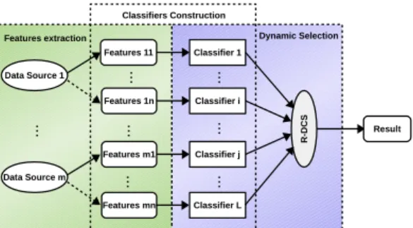
C. R-DCS in multi-sources data classification
We apply the proposed R-DCS model in multi-sources data classification. A framework of multi-sources data classification with R-DCS is illustrated in Figure 2. It involves three blocks: (i) feature extraction from the original data sources; (ii) classifier construction based on the extracted features and (iii) dynamic classifier selection from the classifier pool.
Fig. 1. An illustration of the R-LA strategy. Three green triangles and three purple squares are selected to compute the local accuracy inψ1andψ2.
Fig. 2. Multi-sources data classification with R-DCS.
This general model admits multiple types of features from one or more data sources. In this work, we extract features by applying morphological openings and closings with partial reconstruction on different data sources, similarly as in [16], [17], to generate morphological features.
In particular, for HSI data, spectral features are obtained from the original HSI and spatial features are generated by mathematical morphology. For LiDAR data, elevation features are generated by morphological operators. A separate classifier is constructed for each type of the features. By this, a pool of classifiers is obtained for dynamic selection in the R-DCS model.
IV. EXPERIMENTALRESULTS AND ANALYSIS
We conduct experiments on two real data sets: a HSI data set and a combined HSI and LiDAR data set. We compare the methods Rt and R-LA in our proposed R-DCS model with the following schemes: 1) K-nearest neighbors (KNN) classifier with spectral features of HSI; 2) NBC with different features, i.e. NB-Spe (spectral features in HSI), NB-Spa (morpholog-ical features in HSI) and NB-Ele (morpholog(morpholog-ical features in LiDAR); 3) Generalized graph-based fusion (GGF) [2]. Three widely used performance measures: overall accuracy (OA), average accuracy (AA) and Kappa coefficient (κ) are used for quantitative assessment. In the following experiments, half of the labeled samples are used for training and the rest are for testing. Experimental results are reported in average of 10 runs.
(a) (b) (c) OA=58.17 (d) OA=92.05
(e) OA=65.56 (f) OA=93.29 (g) OA=77.06 (h) OA=93.57 Fig. 3. Indian Pines image. (a) False color image, (b) Ground truth, classification maps of (c) NB-Spe (d) NB-Spa (e) KNN (f) GGF (g) R-DCS with Rt strategy (h) R-DCS with R-LA strategy.
A. Experiments on HSI
We first conduct experiments on Indian Pines, which was gathered by the Airborne/Visible Infrared Imaging Spectrom-eter (AVIRIS) sensors from the North-western Indiana in June 1992. It has a data size of145×145×224 and consists of 16 classes. The morphological features are extracted from the first 3 principal components of the HSI data with 5 opening and closings by using disk-shaped SE (ranging from 2 to 10 with step size increment of 2).
The results reported in Table I and Figure 3 reveal that our method R-LA achieves the best performance. Compared with NB-Spe and NB-spa, our Rt method shows a lower accuracy, which demonstrates that DSC with the highest robustness may not improve the classification performance. In contrast, the proposed R-LA yields an improved performance, which benefits from the adaptive selection of thresholds, ensuring that the classification accuracy of each test pixel is closer to the best result of the nearby pixels. Our method R-LA also obtains a better result than the feature fusion based classification method GGF.
B. Experiments on HSI and LiDAR
The second data set comes from the 2013 IEEE GRSS data fusion contest [18]. We refer to it as GRSS2013. It was acquired over the University of Houston campus and the neighboring urban area in June 2012. It involves two types data sources: an HSI and a LiDAR derived Digital Surface Model (DSM). The HSI has 144 spectral bands and 349 × 1905 pixels. The ground truth provided for this dataset contains 15 classes. The morphological features are generated with the same method in [18].
The results are reported in Table II, Rt does not perform good enough, which proves our assumption again that it does not make sense to directly compare the perturbation thresholds of different classifiers and the combination methods might not always be the best option. However, the proposed R-LA yields again the best performance in terms of OA, AA andκ. Compared with the feature fusion based method GGF,
TABLE I
CLASSIFICATION ACCURACY FORIndian Pines.
NB-Spe NB-Spa KNN GGF Rt R-LA OA(%) 57.48 92.15 63.52 92.95 76.39 93.24 AA(%) 54.71 89.52 47.20 90.11 78.53 90.17 κ 0.5171 0.9107 0.5712 0.9188 0.7304 0.9232 TABLE II
CLASSIFICATION ACCURACY FOR THEGRSS2013DATASET.
Class NB-Spe NB-Spa NB-Ele KNN GGF Rt R-LA 1 96.73 99.94 91.82 96.62 98.51 98.69 99.98 2 96.56 98.55 89.87 95.58 98.84 99.72 99.70 3 92.25 99.06 95.19 95.10 100 96.60 99.04 4 93.99 98.94 97.59 92.72 99.22 98.96 98.98 5 88.05 100 96.70 98.65 100 99.36 100 6 89.88 100 100 72.50 100 98.67 100 7 67.78 99.20 97.90 79.39 100 86.00 99.75 8 47.64 99.19 98.68 62.40 100 89.56 99.66 9 75.77 98.05 92.41 76.03 99.04 86.60 99.17 10 47.48 98.43 90.18 82.82 100 69.73 99.77 11 69.45 97.42 97.16 69.44 98.77 86.21 98.83 12 28.32 100 97.67 65.11 99.59 66.01 99.94 13 19.91 96.57 95.58 0 84.00 65.32 97.81 14 93.54 100 100 86.64 100 99.76 100 15 82.43 100 97.61 92.84 100 97.13 100 OA(%) 72.14 98.33 95.29 80.89 99.11 88.73 99.62 AA(%) 72.65 98.32 95.89 77.72 98.59 89.22 99.60 κ 0.6980 0.9828 0.9489 0.7921 0.9904 0.8776 0.9959
our method offers the robustness to model specification and achieves a better performance at the same time. Moreover, our proposed model is parameter free, which makes it more practical for real applications.
V. CONCLUSION
The main contribution of this work is a novel, robust dy-namic classifier selection method, that we refer to as R-DCS. The experimental results demonstrate that the proposed R-DCS model with the R-LA strategy not only outperforms each of the individual classifiers it is based on, but also achieves a better performance than the feature fusion based classification method GGF. Although the proposed model is computationally very simple, it naturally improves the robustness to model specification without sacrificing the classification accuracy.
ACKNOWLEDGMENT
We acknowledge support for this project from the China Scholarship Council and Research Foundation - Flanders (FWO) under the grant G.OA26.17N.
REFERENCES
[1] W.Liao, F.Van Coillie, L.Gao, L.Li, B.Zhang, and J.Chanussot, “Deep learning for fusion of apex hyperspectral and full-waveform LiDAR remote sensing data for tree species mapping,” IEEE Access, vol. 6, pp. 68716–68729, 2018.
[2] W.Liao, A.Piˇzurica, R.Bellens, S.Gautama, and W.Philips, “Generalized graph-based fusion of hyperspectral and LiDAR data using morpholog-ical features,” IEEE Geoscience and Remote Sensing Letters, vol. 12, no. 3, pp. 552–556, 2015.
[3] H.Li, P.Ghamisi, U.Soergel, and X.Zhu, “Hyperspectral and LiDAR fusion using deep three-stream convolutional neural networks,” Remote Sensing, vol. 10, no. 10, pp. 1649, 2018.
[4] S.Sukhanov, D.Budylskii, I.Tankoyeu, R.Heremans, and C.Debes, “Fu-sion of LiDAR, hyperspectral and RGB data for urban land use and land cover classification,” in IGARSS 2018-2018 IEEE International Geoscience and Remote Sensing Symposium. IEEE, 2018, pp. 3864– 3867.
[5] J.Xia, N.Yokoya, and A.Iwasaki, “Fusion of hyperspectral and LiDAR data with a novel ensemble classifier,” IEEE Geoscience and Remote Sensing Letters, vol. 15, no. 6, pp. 957–961, 2018.
[6] A. L.Brun, A. S.Britto Jr, L. S.Oliveira, F.Enembreck, and R.Sabourin, “A framework for dynamic classifier selection oriented by the classifi-cation problem difficulty,” Pattern Recognition, vol. 76, pp. 175–190, 2018.
[7] R. M.Cruz, R.Sabourin, and G. D.Cavalcanti, “Dynamic classifier selection: Recent advances and perspectives,” Information Fusion, vol. 41, pp. 195–216, 2018.
[8] H.Su, B.Yong, P.Du, H.Liu, C.Chen, and K.Liu, “Dynamic classifier selection using spectral-spatial information for hyperspectral image classification,” Journal of Applied Remote Sensing, vol. 8, no. 1, pp. 085095, 2014.
[9] B. B.Damodaran, R. R.Nidamanuri, and Y.Tarabalka, “Dynamic ensem-ble selection approach for hyperspectral image classification with joint spectral and spatial information,” IEEE J. Sel. Top. Appl. Earth Obs. Remote Sens, vol. 8, no. 6, pp. 2405–2417, 2015.
[10] T. G.Dietterich, “Steps toward robust artificial intelligence,” AI Magazine, vol. 38, no. 3, pp. 3–24, 2017.
[11] A.Fawzi, O.Fawzi, and P.Frossard, “Analysis of classifiers robustness to adversarial perturbations,” Machine Learning, vol. 107, no. 3, pp. 481–508, 2018.
[12] J.De Bock, C. P.De Campos, and A.Antonucci, “Global sensitivity analysis for MAP inference in graphical models,” inAdvances in Neural Information Processing Systems, 2014, pp. 2690–2698.
[13] M.Li, J.De Bock, and G.De Cooman, “Dynamic classifier selection based on imprecise probabilities: A case study for the naive bayes classifier,” in International Conference Series on Soft Methods in Probability and Statistics. Springer, 2018, pp. 149–156.
[14] J.-M.Bernard, “An introduction to the imprecise Dirichlet model for multinomial data,” International Journal of Approximate Reasoning, vol. 39, no. 2-3, pp. 123–150, 2005.
[15] M.Zaffalon, “The naive credal classifier,”Journal of statistical planning and inference, vol. 105, no. 1, pp. 5–21, 2002.
[16] M.Pesaresi and J. A.Benediktsson, “A new approach for the morphologi-cal segmentation of high-resolution satellite imagery,”IEEE transactions on Geoscience and Remote Sensing, vol. 39, no. 2, pp. 309–320, 2001. [17] S.Jia and J.Xian, “Multi-feature-based decision fusion framework for hyperspectral imagery classification,” in IGARSS 2018-2018 IEEE International Geoscience and Remote Sensing Symposium. IEEE, 2018, pp. 5–8.
[18] “2013 ieee grss data fusion contest,” http://www.grss- ieee.org/community/technical-committees/data-fusion/2013-ieee-grss-data-fusion-contest/.