NOTES AND CORRESPONDENCE
Interaction of Mesoscale Variability with Large-Scale Waves in the Argentine Basin
LEE-LUENGFU
Jet Propulsion Laboratory, California Institute of Technology, Pasadena, California
(Manuscript received 24 July 2005, in final form 13 April 2006) ABSTRACT
The Argentine Basin of the South Atlantic Ocean is a region of complicated ocean dynamics involving a wide range of spatial and temporal scales. Previous studies reported the existence of a basin mode of topographic barotropic Rossby waves with a period close to 25 days in the region. Using observations of sea level anomalies from satellite altimeter measurements, the present study provides evidence of interaction between the large-scale 25-day waves and the energetic mesoscale variability of the region. The amplitude of the 25-day waves is highly intermittent with dominant periods in the range of 110–150 days. Within this period band, the wave amplitude is coherent with the energy level of the mesoscale variability: when the mesoscale energy level goes down, the wave amplitude goes up, and vice versa, suggesting an exchange of energy between the two scales. This coherence is linked to the first three empirical orthogonal functions (EOFs) of the sea level anomalies. The spatial patterns of these EOFs are characterized by eddies and meanders associated with the Brazil–Malvinas Confluence. The findings of the study suggest a mechanism of energy exchange at work between the mesoscale variability and the large-scale waves in the Argentine Basin.
1. Introduction
The Argentine Basin of the South Atlantic Ocean is a region where the ocean circulation exhibits complex patterns of mean flow and variability. The confluence of the Malvinas Current with the Brazil Current is one of the most energetic current systems of the world’s oceans, creating meanders and eddies that effectively mix the different water masses carried by the two cur-rents (Olson et al. 1988; Garzoli and Garraffo 1989; Matano et al. 1993; Provost and Le Traon 1993; Sa-raceno et al. 2004). In the center of the basin there is an intense anticyclonic gyre of barotropic circulation transporting water at a rate of 140 Sv (1 Sv ⬅ 106
m3s⫺1) around the Zapiola Rise, a sediment ridge at
the ocean’s bottom (Saunders and King 1995; de Miranda et al. 1999). Superimposed on the gyre are rapidly rotating barotropic waves around the Zapiola
Rise with a period close to 25 days (Fu et al. 2001). These dynamical processes of wide-ranging spatial and temporal scales make the Argentine Basin a uniquely interesting place to explore the interactions of ocean variability at different scales.
Based on sea surface height observations from satel-lite altimetry, Fu et al. (2001) illustrated that the 25-day waves were barotropic topographic Rossby waves caused by the sloping bottom around the Zapiola Rise. The waves represent the gravest mode of the basin with closedf/Hcontours, wherefis the Coriolis parameter andHis water depth. They have a dipolar pattern ro-tating counterclockwise around the Zapiola Rise. The spatial scale of the dipole is about 1000 km. A new calculation based on improved methods of mapping al-timeter data leads to a typical peak-to-trough ampli-tude of 20 cm for the waves (Tai and Fu 2005). The findings based on satellite altimetry have been con-firmed by in situ observations made by bottom pressure recorders (Hughes et al. 2007).
Although the 25-day waves are a persistent feature of the region throughout the decade-long Ocean Topog-raphy Experiment (TOPEX)/Poseidon (T/P) altimeter data record, the magnitude of the wave amplitude is
Corresponding author address:Lee-Lueng Fu, Jet Propulsion Laboratory, MS 300-323, 4800 Oak Grove Drive, Pasadena, CA 91109.
E-mail: [email protected] DOI: 10.1175/JPO2991.1
© 2007 American Meteorological Society
between adjacent T/P ground tracks is about 200 km at midlatitudes, and thus is not suitable for resolving the mesoscale eddies. The high-resolution data produced by the Archiving, Validation, and Interpretation of Sat-ellite Oceanographic Data (AVISO) project using al-timeter data from multiple satellites (Ducet et al. 2000) are used for analyzing the eddy energy in the study.
2. Ocean variability at two scales
The AVISO Maps of Sea Level Anomaly (MSLA) data product is based on the altimeter data from the T/P,Jason,European Remote Sensing Satellite(ERS)-1 and -2, and Environment Satellite (ENVISAT) mis-sions (information available online at ftp://ftp.cls.fr/ pub/oceano/enact/msla/readme_MSLA_ENACT.htm). The data are provided weekly on grids whose meridi-onal and zmeridi-onal grid sizes are equal to the distance of 1/3 of a degree of local longitude (e.g., from 37 km at the equator to 18.5 km at 60°N/S). The duration of the data record used for the study spanned from October 1992 to July 2004. There are no ERS data between January 1994 and March 1995 (ERS-1geodetic phase). TOPEX/Poseidon was replaced by Jason in August 2002 after its orbit change (with ground tracks inter-leaved with those ofJason).ERS-2was available from June 1996 to June 2003, after which it was then replaced by ENVISAT.
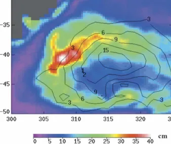
Displayed in Fig. 1 is the standard deviation of the sea level anomaly (SLA) based on the MSLA record. Also shown is the maximum sea level amplitude of the large-scale 25-day waves derived from the new mapping procedure of Tai and Fu (2005). The SLA variability is dominated by the energy at the mesoscales (Ducet et al. 2000). Figure 2 shows the correlation between two SLA time series along 40°S as a function of their spatial sepa-ration. The correlation, denoted asCx(s), wherexis the
longitude andsis the distance between two SLA time serieshxandhx⫹s, is computed as follows:
Cx共s兲⫽ 具hxhx⫹s典
公
具hx 2 典具hx⫹s 2 典.What is shown in Fig. 2 is the zonal average ofCx(s) for
each distances. Denoting the zonal average asC(s), a spatial scaleLis then computed as follows:
L⫽
冕
⫺⬁ ⬁
关C共s兲兴2dsⲐ关C共0兲兴2.
The value ofLestimated from above is 212 km, con-firming that the SLA is dominated by the mesoscale energy. Note that the 25-day waves, whose spatial scale is 1000 km, are obtained after the mesoscale energy is removed from the T/P data used by Fu et al. (2001). The geographical distributions of the energy at the two different scales, however, have significant overlap. The question is whether there is a relationship between the variabilities at the two scales.
FIG. 2. The temporal correlation of the sea level anomaly as a function of the distance of separation.
FIG. 1. Color map: The standard deviation of the sea level anomaly. Contours: The maximum amplitude of the 25-day waves (cm).
3. The temporal relations between the two scales
The variability of the 25-day waves was first investi-gated. Following Fu et al. (2001), the spatially low-passed T/P data in the region bounded by 30°–50°S, 300°–335°E were high-pass filtered in time to remove the variance at periods longer than 30 days. A complex-valued empirical orthogonal function (CEOF) analysis was then performed on the high-passed data. Each mode of the CEOF is expressed as A(x, y)B(t) exp{i[C(x,y)⫹D(t)]}, wherex,yrepresent the spatial location and t represents time. Shown in Fig. 3 is the time series of the amplitudeA(x,y)B(t) of the leading CEOF (accounting for 40% of the high-passed vari-ance) at 40°S, 315°E, where the energy of the 25-day waves represented by the CEOF is maximum. As noted in Fu et al. (2001) there is a high degree of intermit-tency in the temporal variability of the amplitude of the 25-day waves. Figure 4a shows its variance-preserving spectrum. Although the variance is spread over a wide range of frequencies, the main lobe of the distribution is located at periods from 100 to 160 days, which are considered the dominant time scales of the variability. Another measure of the time scale is made from the autocorrelation of the time series as
T⫽
冕
⫺⬁ ⬁
关C共兲兴2dⲐ关C共0兲兴2,
where T is the time scale, C() is the autocorrelation function, andis a time lag. HereTis estimated to be 130 days, confirming that the time scales of the vari-ability are in the mesoscale range. Is the varivari-ability of the wave amplitude related to the variability of the me-soscale energy level in the region? The spatial variance of SLA was then computed over the entire domain at weekly intervals to represent a time series of the me-soscale energy level. Shown in Fig. 4b is the
variance-preserving spectrum of the mesoscale energy time se-ries. The distribution of the variance of the mesoscale energy level is also spread over a wide range of fre-quencies, with the majority in the seasonal-to-interannual range. However, there is significant vari-ance at higher frequencies, including the range corre-sponding to periods of 100–160 days.
To investigate possible relationships between the wave amplitude and the mesoscale energy level, the coherence between the two time series was computed (Fig. 5). The level of coherence at periods of 110–150 days is significantly above zero at 95% confidence (Koopmans 1974). The phase varies from ⫺150° to
⫺190° (⫺190° is equivalent to 170° in the plot), which is not distinguishable from⫺180° at the 95% confidence level (Koopmans 1974). The information from the co-herence and phase suggests that there is a linear rela-tion between the wave amplitude and the level of me-soscale energy in the period band of 110–150 days. To FIG. 3. The variation of the amplitude of the 25-day waves at
40°S, 315°E from 1993 to 2002.
FIG. 4. Variance-preserving spectrum of (a) the magnitude of the amplitude of the 25-day waves, and (b) the variance of sea level anomaly. The units are arbitrary.
further illustrate the relation, Fig. 6 shows a scatterplot of the SLA variance versus the wave amplitude after the two time series were filtered to retain variance only in the period band of 110–150 days. The substantial scatter reflects the rather marginal coherence, but the overall pattern reveals the following relationship: the wave amplitude goes up when the SLA variance goes down and vice versa, suggesting an exchange of energy between the two scales. Note that the time mean is removed from both time series in the filtering opera-tion; the values of the variance and amplitude are ref-erenced to their means, and hence have both positive and negative values.
Because the SLA variance also includes the variance associated with the 25-day waves, albeit a minute por-tion, one might wonder whether the apparent coher-ence is caused by the signal of the waves itself. To examine this possibility, I also computed the coherence between the wave amplitude and the variance of the spatially low-passed data from which the 25-day waves
were derived. There was no significant coherence at any frequencies (not shown). Therefore, the coherence at periods of 110–150 days is indeed attributable to the presence of the mesoscale variability and its interaction with the large-scale waves.
4. Spatial and temporal characteristics of the interaction
What is the part of the mesoscale variability respon-sible for the coherence with the 25-day waves? An em-pirical orthogonal function (EOF) analysis was applied to the MSLA data. The amplitude of each mode was analyzed for its coherence with the amplitude of the 25-day waves (Fig. 7a). The first three modes, account-ing for 18.3% of the variance collectively, are signifi-cantly coherent with the wave amplitude in a period band centered on 110 days, and with a stable phase over a wide range of frequencies (not shown). Figure 7b shows that the coherence exhibited in Figs. 5 and 6 is indeed linked to the first three modes, because the co-herence already reaches its final value (0.65) when the SLA is constructed using only the first three modes. The coherence and phase at all frequencies are shown in Fig. 8. Compared to Fig. 5, by retaining only the first three EOF modes, the coherence becomes significant over a broader range of frequencies and the phase be-comes more stable at low frequencies. Note the sharp transition from the stable to noisy phase at periods just shorter than 100 days. The higher-order modes, appar-ently not interacting with the 25-day waves, simply add noise and degrade the coherence calculation shown in Fig. 5.
Displayed in Fig. 9 are the spatial patterns of the first FIG. 5. (top) Coherence and (bottom) phase (°) of the
ampli-tude of the 25-day waves with the variance of the sea level anomaly. The 95% confidence level of nonzero coherence is shown.
FIG. 6. The SLA variance vs the amplitude of the 25-day waves
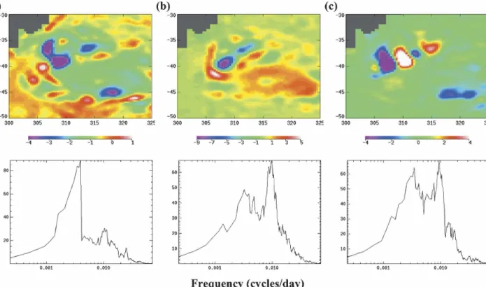
three EOF modes and the frequency spectra of their amplitudes. The first two modes exhibit both gyre-scale and mesoscale variability, while the third mode shows only the mesoscale. The first mode’s variance is primar-ily associated with periods longer than 250 days with significant annual variability. The second and third modes involve a broader range of frequencies. It seems that the first two modes represent some covariability of both the gyre scale and mesoscale, while the third mode strictly involves the mesoscale variability associated with the meander and eddy shedding of the currents of the Brazil—Malvinas Confluence. As noted earlier, when the three modes are added together, the resultant sea level anomalies exhibit a linear relationship be-tween the sea level variance and the amplitude of the 25-day waves in the period band of 110–150 days. The
standard deviation of the sea level anomalies from the three EOF modes (Fig. 10) has a spatial pattern basi-cally similar to that of the total signal (Fig. 1), with a much-reduced magnitude. There seems to be an inter-action between the large-scale waves with the meso-scale variability in the proximity of the Brazil–Malvinas Confluence.
5. Discussion
As described in Fu et al. (2001), the 25-day waves in the Argentine Basin are a manifestation of a normal mode of the basin associated with the Zapiola Rise. Because the mode is near a resonance of the basin, it can be excited by a variety of sources and easily simu-lated by a numerical model with the right geometry and resolution. The simulations performed by a barotropic model reported in Fu et al. (2001) reproduced both the spatial pattern and the time scales of the waves quite well. The model has a resolution of 50 km, which is not able to resolve the mesoscale eddies. Driven by daily wind, the model was not able to reproduce the temporal evolution of the amplitude of the waves.
The present study provides evidence of the interac-FIG. 7. (a) Coherence of the 25-day wave amplitude with the
amplitude of each EOF (the abscissa is the mode number) at the period of 110 days. Only the first three modes are important. (b) Coherence of the 25-day wave amplitude with the sea level anomaly variance based on the reconstruction using EOFs from mode 1 through the mode number shown by the abscissa. Dashed lines represent the 95% confidence levels.
FIG. 8. (top) Coherence and (bottom) phase (°) of the 25-day wave amplitude with the sea level anomaly variance summed from the first three EOF modes.
tion between the 25-day waves and the mesoscale vari-ability of the basin. Within the period band of 110–150 days, which is the dominant time scale of the wave amplitude variability, the mesoscale energy level is
lin-early related to the wave amplitude. When the meso-scale energy goes down, the wave amplitude goes up, and vice versa, suggesting an exchange of energy be-tween the mesoscale and the large scales (⬃1000 km) of the waves.
The coherence between the mesoscale variability and the large-scale waves is linked to the first three leading EOFs of the sea level variability. Although the coher-ence is only marginally significant, its frequency range becomes wider and the phase becomes more stable when only the first three EOFs are retained in the me-soscale variability. Apparently, the higher-order com-ponents of the mesoscale variability are not interacting with the large-scale waves, and their presence degrades the significance of the coherence.
The spatial patterns of the first three EOFs of the sea level variability are quite complex. The temporal vari-ability of each of them is significantly coherent with the amplitude of the large-scale waves. The physical mechanism of the interaction is not clear. The spatial scales of the first two modes have both gyre-scale and mesoscale components, but the third mode is domi-nated by the mesoscale. It represents the meander and eddy shedding of the currents associated with the Bra-zil–Malvinas Confluence. The eddies and meanders of the currents in the region move circularly in a counter-FIG. 10. Color map: The standard deviation of the sea level
anomaly constructed from the first three EOF modes filtered to the 110–150-day period band. Contours: The maximum amplitude of the 25-day waves (cm).
FIG. 9. (top) The spatial patterns of the first three EOFs of the sea level anomaly data: (a) first mode (8.5% variance), (b) second mode (5.2% variance), and (c) third mode (4.6% variance). (bottom) The corresponding variance-preserving spectra of the mode’s amplitude time series are shown. All units are arbitrary.
clockwise direction (Fu 2006). Although this is the same direction as the propagation of the 25-day waves, it is not clear if it is essential for the interaction between the waves and the eddies.
The apparent energy exchange between baroclinic eddies and large-scale barotropic waves probably in-volves a nonlinear energy transfer mechanism. Theo-retically, it is possible to have a group of resonantly interacting waves involving two baroclinic waves and a barotropic wave (Fu and Flierl 1980). Energy is ex-changed among the components of such a triad. Wheth-er a similar mechanism can be at work in the present setting is a topic of theoretical investigation.
The geographic configuration of the various elements of the ocean circulation in the Argentine Basin can be delineated by the letter “C.” The Brazil Current and the Malvinas Current and their confluence are located on the letter proper, as are the eddies and meanders, which move counterclockwise along the letter. The me-soscale energy is essentially confined to the rim of the region represented by the letter (Fig. 1). Situated inside the region surrounded by the letter are the Zapiola anticyclone and the 25-day waves, which circulate and propagate counterclockwise, respectively. It is likely that these elements of the circulation in the region in-teract with one another, leading to the rather unique letter C configuration. The eddies only exist on the rim of the C, while the center of the region seems to be a sink of mesoscale energy. As noted in the introduction, the Argentine Basin is a region of complex variability involving a wide range of scales. More theoretical and modeling studies are required to unravel the complex-ity of the underlying ocean dynamics of the region.
Acknowledgments.The research presented in the pa-per was carried out at the Jet Propulsion Laboratory, California Institute of Technology, under a contract with the National Aeronautics and Space Administra-tion. Support from the TOPEX/Poseidon and Jason Projects is acknowledged.
REFERENCES
de Miranda, A. P., B. Barnier, and W. K. Dewar, 1999: On the dynamics of the Zapiola Anticyclone.J. Geophys. Res.,104,
21 137–21 150.
Ducet, N., P. Y. Le Traon, and G. Reverdin, 2000: Global high resolution mapping of ocean circulation from the combina-tion of TOPEX/Poseidon andERS-1/2. J. Geophys. Res.,105
(C8), 19 477–19 498.
Fu, L.-L., 2006: Pathways of eddies in the South Atlantic Ocean revealed from satellite altimeter observations.Geophys. Res. Lett.,33,L14610, doi:10.1029/2006GL026245.
——, and G. R. Flierl, 1980: Nonlinear energy and enstrophy transfers in a realistically stratified ocean. Dyn. Atmos. Oceans,4,219–246.
——, B. Cheng, and B. Qiu, 2001: 25-day period large-scale oscil-lations in the Argentine Basin revealed by the TOPEX/ Poseidon altimeter.J. Phys. Oceanogr.,31,506–517. Garzoli, S. L., and Z. Garraffo, 1989: Transports, frontal motions
and eddies at the Brazil-Malvinas confluence as revealed by inverted echo sounders.Deep-Sea Res.,36,681–703. Hughes, C. W., V. N. Stepanov, L.-L. Fu, B. Barnier, and G. W.
Hargreaves, 2007: Three forms of variability in Argentine Basin ocean bottom pressure.J. Geophys. Res.,112,C01011, doi:10.1029/2006JC003679.
Koopmans, L. H., 1974:The Spectral Analysis of Time Series. Aca-demic Press, 366 pp.
Matano, R. P., M. G. Schlax, and D. B. Chelton, 1993: Seasonal variability in the southwestern Atlantic.J. Geophys. Res.,98,
18 027–18 035.
Olson, D. B., G. P. Podesta, R. H. Evans, and O. B. Brown, 1988: Temporal variations in the separation of Brazil and Malvinas Currents.Deep-Sea Res.,35,1971–1990.
Provost, C., and P.-Y. Le Traon, 1993: Spatial and temporal scales in altimetric variability in the Brazil-Malvinas Current con-fluence region: Dominance of the semiannual period and large spatial scales.J. Geophys. Res.,98,18 037–18 051. Saraceno, M., C. Provost, A. R. Piola, J. Bava, and A. Gagliardini,
2004: Brazil Malvinas Frontal System as seen from 9 years of Advanced Very High Resolution Radiometer data.J. Geo-phys. Res.,109,C05027, doi:10.1029/2003JC002127. Saunders, P. M., and B. A. King, 1995: Bottom currents derived
from a shipborne ADCP on the WOCE Cruise A11 in the South Atlantic.J. Phys. Oceanogr.,25,329–347.
Tai, C.-K., and L.-L. Fu, 2005: 25-day period large-scale oscilla-tions in the Argentine Basin revisited.J. Phys. Oceanogr.,35,