A Novel Ensemble Method for Imbalanced Data Learning: Bagging of Extrapolation-SMOTE SVM

(1)

Research Article

A Novel Ensemble Method for Imbalanced Data Learning:

Bagging of Extrapolation-SMOTE SVM

Qi Wang, ZhiHao Luo, JinCai Huang, YangHe Feng, and Zhong Liu

Science and Technology on Information Systems Engineering Laboratory, College of Information System and Management, National University of Defense Technology, Changsha, Hunan, China

Correspondence should be addressed to JinCai Huang; huangjincai [email protected]

Received 4 December 2016; Revised 23 December 2016; Accepted 28 December 2016; Published 30 January 2017 Academic Editor: Elio Masciari

Copyright © 2017 Qi Wang et al. This is an open access article distributed under the Creative Commons Attribution License, which permits unrestricted use, distribution, and reproduction in any medium, provided the original work is properly cited.

Class imbalance ubiquitously exists in real life, which has attracted much interest from various domains. Direct learning from imbalanced dataset may pose unsatisfying results overfocusing on the accuracy of identification and deriving a suboptimal model. Various methodologies have been developed in tackling this problem including sampling, cost-sensitive, and other hybrid ones. However, the samples near the decision boundary which contain more discriminative information should be valued and the skew of the boundary would be corrected by constructing synthetic samples. Inspired by the truth and sense of geometry, we designed a new synthetic minority oversampling technique to incorporate the borderline information. What is more, ensemble model always tends to capture more complicated and robust decision boundary in practice. Taking these factors into considerations, a novel ensemble method, called Bagging of Extrapolation Borderline-SMOTE SVM (BEBS), has been proposed in dealing with imbalanced data learning (IDL) problems. Experiments on open access datasets showed significant superior performance using our model and a persuasive and intuitive explanation behind the method was illustrated. As far as we know, this is the first model combining ensemble of SVMs with borderline information for solving such condition.

1. Introduction

In the domain of machine learning, data is essential for the model’s training. However, the distribution of two classes behaves in extremely imbalanced way and the circumstance is quite ubiquitous in real life [1]. In this paper, we concentrate on the binary classification problems when there is extremely imbalanced distribution in two classes; that is, one class for training severely outnumbers the other.

With the neglect of the class imbalanced distribution, tra-ditional algorithms for binary classification tend to perform badly on the dataset [2, 3], leading to the unsatisfied subopti-mal result [4–7] that the majority class can be well identified while the minority is reverse. One of the reasons accounting for this is that the imbalanced distribution as prior infor-mation in many instances has a strong impact on final dis-crimination [8]. Now let us consider a special scenario in which the majority class amounts to the percentage of 99. In such case, an ordinary classifier that assigns any example to the majority class label would still achieve the accuracy of

99% [9]. However, due to the low recall ratio for the minority, such extreme result is not what we have desired. The phe-nomena are quite crucial and nontrivial in several circum-stances, such as identification of network intrusion [10, 11], medical diagnosis of type 2 diabetes [12], oil spills detection from satellite radar images [13], finding of financial fraud transactions [14], and bioinformatics [15]. Another fact which cannot be neglected is that in most of the binary classification problems, the minority class is what we really care about rather than the majority [3], especially when the cost is expensive for the failure in recognizing the minority ones.

Numbers of algorithms have been designed for relieving the consequences of the imbalanced data. From the perspec-tive of the strategy, these methods can be categorized as three mainstream types. In the algorithm level, the adjustment of the weights of errors in the loss function, also called cost-sensitive learning, is a direct way to reduce the impact of imbalance. Cost matrix which measures different penalties for misclassification is critical for the improvement on the performance. Another way to tune the penalties was rooted https://doi.org/10.1155/2017/1827016

(2)

in adaptive boosting [16] and some algorithms, for example, Ada-cost [17] and cost-sensitive boosting [18], were imple-mented for the learning task. In the sampling level, the easiest way is to randomly sample the training data from the whole training dataset in the way that different classes of data are sampled in appropriate ratios to balance the proportions in classes. Random sampling tended to be overfitting if the pling ratios were not properly modulated [3]. Repeated sam-pling was easier to implement but hard to adjust efficiently, so Provost [9] thought undersampling was proper for the larger training dataset while the synthetic samples were constructed for the less sample cases. Estabrooks et al. [2] combined different repeated sampling methods to offer a better scheme of modulation. Another popular method was the synthetic minority oversampling technique (SMOTE) proposed by Chawla et al. [19] and the core idea was to construct the syn-thetic minority samples through the interpolation between minority training data and its 𝑘-nearest neighborhoods. Han et al. [3] paid more attention to the samples near the decision borderline and combined the SMOTE to acquire the Borderline-SMOTE. Apart from the above sampling methods, clustering-based resampling algorithm [20] and SMOTE-Boost algorithm [21] were also designed for the imbalanced cases. Furthermore, fewer researchers focused on how the sampling methodologies impact on the learning performance but the reason why sampling methods boost the linear discriminative performance was given by Xue and Hall [6].

In addition to the algorithm and sampling based meth-ods, other researchers proposed several practical and popular methods with excellent performance from the hybrid view. With the help of SMOTE on the boundary samples and the adjustment of kernel matrix, Wu and Chang [22] integrated the prior information of distribution of imbalance with SVM to obtain the kernel boundary alignment algorithm. Chawla et al. [4] noticed the great influence of feature selection and Maldonado et al. [23] did some research on various ways of feature selection and put forward backward elimination feature selection process for SVM’s dealing with the IDL problem. Two-stage cost-sensitive learning was employed in the NASA imbalanced data and the researcher designed cost-sensitive rules for both feature selection and the classification stage [24]. Rather than former over- or undersampling meth-ods, Sun et al. [25] utilized random partition and clustering tricks to obtain some balanced datasets for training various classifiers and combined them according to some rules. Bhowan et al. made use of genetic programming to construct types of fitness functions and exploit the multiobjective opti-mization for combining the classifiers [5]. Easy ensemble and balance cascade [26] were two superior algorithms, which made use of ensemble models learned in an undersampling way.

Quite different from the above-mentioned methods, we would propose a novel ensemble algorithm, in which an efficient sampling method was developed for IDL problems. Necessarily, similar works are summarized as follows. In the preprocessing process, Batuwita and Palade [27] screened some informative examples closer to the class boundary captured by SVM and downscaled the resampling of other

samples to reduce the time complexity of training SVM with performance maintained. For the binary imbalanced data, Wu and Chang implemented boundary alignments using kernel tricks to relieve the offset of decision boundary [28]. From the perspective of ensemble, there exist several elab-orate reviews about ensemble models for the IDL [8, 29]. Specifically, L´opez et al. [8] studied how six significant prob-lems relating to the data intrinsic characteristics affected the performance of ensemble models for the IDL. Several supe-rior ensemble models are based on boosting, such as EUS-Boost [30], evolutionary undersampling boosting model in dealing with breast cancer malignancy classification [31]. Shi et al. made use of bagging technique on SVM to cope with P300 detection problem [32]. Our proposed framework also made use of those samples near the decision boundary detected by the SVM but in a more flexible way of sampling. We applied bagging technique to meta-SVM trained with data obtained from the sampling process. The final results show our model’s effectiveness in dealing with the IDL problem.

2. Materials and Methods

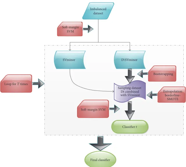
Before our framework was introduced, some basic knowledge about models or techniques would be in a brief summary. In our framework, SVM works as metaclassifiers for ensemble and bootstrapping aggregation is a type of sampling tech-nique to obtain various training dataset. Besides, we would illustrate SMOTE in a comprehensive way and induce our adaptive SMOTE technique. Flow chart about our framework is given in Figure 1.

2.1. Support Vector Machine: A Review. Support vector mach-ine as one of the popular classifiers in binary classification has shown its state of art performance in engineering appli-cations.

Given the labeled training set𝑇 = {(x_i, 𝑦_𝑖) | 𝑦_𝑖= 1or−1, 𝑖 = 1 ⋅ ⋅ ⋅ 𝑁}, a na¨ıve idea to learn a classifier is to characterize a hyperplane in the feature or transformed feature space of the inputxthat can separate two classes of training data as much as possible. Based on the statistical learning theory [33], SVM is recognized as the robust adaptation for the perceptron learning model [34].

Trick of feature transformation𝜙and soft-margin relax-ation make SVM powerful for the detection of complex deci-sion boundary and control the overfitting with the allowance for some samples’ violating the support hyperplanes.

Here, we give an expression of SVM in the form of quadratic programming problem as follows:

min 𝑊,𝑏,𝜁 1 2𝑊𝑇∗ 𝐼𝑛∗ 𝑊 + 𝐶 (1𝑇𝑁∗ 𝜁) s.t 𝐴 ( 𝑊 𝜁 𝑏 ) ≥ 1_𝑁, (1)

(3)

Imbalanced dataset SVminor D\SVminor Sampling dataset Dt combined with SVminor Classifier t Bootstrapping Extrapolation borderline-SMOTE Soft-margin SVM

Loop for _T times

Final classifier Soft-margin

SVM

Figure 1: The flowchart of our proposed framework.𝐷is the complete dataset and SVminor is the support vectors in the minority after the initialized SVM’s detection.

where𝐴is the corresponding matrix

𝐴 = (( ( 𝑦₁𝜙 (𝑥₁)𝑇, 𝜖₁, 1 𝑦₂𝜙 (𝑥₂)𝑇, 𝜖₂, 1 ... 𝑦_𝑁𝜙 (𝑥_𝑁)𝑇, 𝜖_𝑁, 1 ) ) ) . (2)

𝑁-dimension unit vector𝜖_𝑘with𝑘th coordinate equals 1. The slacked vector of variables 𝜁 = (𝜁₁, 𝜁₂, . . . , 𝜁_𝑁)𝑇 mea-sures the extent to samples’ violating the support hyperplanes. The primal problem can be converted to the dual one by solving the Karush-Kuhn-Tucker optimal functions derived from the Lagrange equation [35].

Finally, the discriminative function is obtained in the form

𝑓 (𝑥) =sign( ∑

𝛼∗ 𝑛>0

𝑦_𝑛𝛼∗_𝑛𝜙 (𝑥_𝑛)𝑇∗ 𝜙 (𝑥) + 𝑏) , (3)

where 𝛼_𝑛∗ is the Lagrange multiplier corresponding to the sample satisfying Karush-Kuhn-Tucker (KKT) optimal con-ditions.

Specifically, when the inner product of the transformed feature vectors can be applied with the kernel methods, the process of computation is efficient:

𝜙 (𝑥_𝑛)𝑇∗ 𝜙 (𝑥_𝑚) = 𝐾 (𝑥_𝑛, 𝑥_𝑚) . (4) Furthermore, only a small proportion of the training data corresponding to positive Lagrange multipliers called support vectors are useful for the final decision, so the representation of the classifier is rather sparse.

2.2. Ensemble Methods: A Review. Apparently one classifier may be severely affected when the training dataset cannot well characterize the actual underlying distribution or the presumed model is biased. The strategy of models’ ensemble can avoid the one-sidedness originated from the training dataset and hypothesis, receiving a better capability of gen-eralization. In another aspect, weaker classifiers are easier to

(4)

(1) Input the whole training dataset with|𝐷| = 𝑁 (2) For𝑖from 1 to𝑚:

(3) Sample from𝐷by Bootstrapping trick to obtain𝐷_𝑖with|𝐷_𝑖| = 𝑁∼ (4) Derive the model𝑓_𝑖(𝑥)by fitting𝐷_𝑖

(5) Ensemble of the models{𝑓_𝑖(𝑥) | 𝑖 = 1, 2, . . . , 𝑚}and obtain the final model𝐹(𝑥). In binary classification cases,𝐹(𝑥) =sign(∑_{𝑖=1,2,...,𝑚}𝑓_𝑖(𝑥))

Algorithm 1: Bagging algorithm.

obtain using simple criteria like stump and a strong classifier can be derived by combining multiple weaker classifiers [36]. In our proposed framework for the IDL, bagging technique was employed for developing various models.

Bootstrapping aggregation abbreviated as bagging con-structs totally different classifiers based on the bootstrap-ping method. Bootstrapbootstrap-ping technique samples each training example in the same probability with replacements.

The general bagging algorithm can be described as shown in Algorithm 1.

One of the most famous models motivated from bagging is random forest in which not only is the training data sam-pled in bootstrapping way, but the features for training are selected in random as well [37]. Table 1 provides a detailed process of sampling methods.

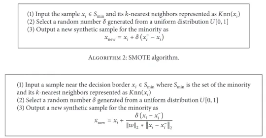
2.3. Bagging of Extrapolation Borderline-SMOTE SVM 2.3.1. Extrapolation Borderline-SMOTE. For IDL, SMOTE [19] is a typical oversampling method with universal appli-cations and the concrete process for generating the synthetic samples can be described as shown in Algorithm 2.

Generating some synthetic samples for the minority in an interpolation way is demonstrated to be effective for relieving the extent of imbalance and lifting performance. However, it seems that samples near the decision border overweigh the remaining ones in decision-making. Borderline-SMOTE [3] operates on samples near the decision border using SMOTE technique. Figure 2 displays the interpolation method to generate synthetic samples.

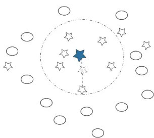
However, the interpolation between samples used in SMOTE or Borderline-SMOTE restricts the ability of explor-ing towards the actual boundary. As we would make use of ensemble SVMs, samples near decision boundary can be roughly characterized from support hyperplane learned by the first SVM. Taking this into consideration, a novel syn-thetic minority oversampling method is proposed as shown in Algorithm 3 and Figure 3 describes our ideology.

Here1/‖𝑤‖₂is the distance from support hyperplane to decision hyperplane corresponding to the first SVM learned from the imbalance training dataset.

It is obvious that the synthetic minor sample tends to correct the skew finely and the extrapolation works to detect the decision boundary when𝑥∼_𝑖 belongs to the inner side of support hyperplane just as Figure 3 indicates.

Figure 2: Manipulation of SMOTE. Stars stand for the minority and the solid star is selected for SMOTE. Circles are the majority. The selected sample randomly picks up one sample from it𝑘-nearest neighbors to interpolate a synthetic sample labeled as the minority.

Support hyperplane

Discriminating hyperplane Synthetic sample

Figure 3: The effect of Extrapolation Borderline-SMOTE. X with no frame is the sample belonging to the minority after Extrapolation Borderline-SMOTE. A synthetic sample labeling to the minority explores towards the actual boundary and it seldom violates the original decision boundary with the help of𝛿.

2.3.2. Bagging of Extrapolation Borderline-SMOTE SVM.

Ensemble methods can effectively enhance model’s capability of generalization. Here, a novel ensemble method for solving IDL problems is proposed called Bagging of Extrapolation Borderline-SMOTE SVMs (BEBS).

(5)

(1) Input the sample𝑥_𝑖∈ 𝑆_minand its𝑘-nearest neighbors represented as𝐾nn(𝑥_𝑖) (2) Select a random number𝛿generated from a uniform distribution𝑈[0, 1] (3) Output a new synthetic sample for the minority as

𝑥_new= 𝑥_𝑖+ 𝛿 (𝑥∼

𝑖 − 𝑥𝑖)

Algorithm 2: SMOTE algorithm.

(1) Input a sample near the decision border𝑥_𝑖∈ 𝑆_minwhere𝑆_minis the set of the minority and its𝑘-nearest neighbors represented as𝐾nn(𝑥_𝑖)

(2) Select a random number𝛿generated from a uniform distribution𝑈[0, 1] (3) Output a new synthetic sample for the minority as

𝑥new= 𝑥𝑖+ 𝛿 (𝑥𝑖− 𝑥

∼

𝑖)

‖𝑤‖2∗ 󵄩󵄩󵄩󵄩𝑥𝑖− 𝑥∼𝑖󵄩󵄩󵄩󵄩2

Algorithm 3: Extrapolation Borderline-SMOTE algorithm.

For SVM, it is noted that support vectors with positive Lagrange multipliers decide the final discriminative bound-ary. So we employ Extrapolation Borderline-SMOTE to the support vectors belonging to the minority for relieving the imbalance level.

The whole ideas about BEBS can be elucidated as follows. The original support vectors containing borderline informa-tion are roughly identified through the base SVM which is learned from the imbalance dataset𝐷. During the initial-ization process, a proper kernel and hyperparameter𝐶are chosen through cross-validation in which G-means is chosen as the optimal metrics. Then the original support vectors belonging to the minority are marked as SV₀ = {𝑥(0)_SV𝑖}and a novel dataset𝐷∼ = 𝐷 \SV₀ for further bootstrapping is constructed by removing SV₀. Bootstrapping is performed on 𝐷∼ in 𝐾-turns and each sampling result 𝐷∼_𝑡 is in the scale of |𝐷∼|. Furthermore, aggregating datasets of 𝐷∼_𝑡and SV₀are operated by Extrapolation Borderline-SMOTE. After that, the merged datasets with new synthetic samples are used for meta-SVM’s training and the original data which are not sampled work as validation sets for tuning parameters. Finally,𝐾SVMs are aggregated in the same weight to form the ensemble classifier (see Algorithm 4).

Specifically, default parameters in our model were initially set as𝛼 = 0.5, 𝐾 = 100and the following experiments shared the same parameters.

2.3.3. The Intuition behind BEBS. The core idea of BEBS is to aggregate various SVMs which revise the initial deci-sion boundary by constructing synthetic minority samples towards the correct direction. These synthetic samples are presumed to well characterize the actual decision boundary. The SVMs’ variance originates from two sources. One is the random selection from SV₀with the sampling ratio𝛼% and the other originates from training sets’ difference due to boot-strapping manipulation. Besides, training data not sampled in a trek of bootstrapping is exploited as the validation set for exploring a better hyperparameter; just see Table 1. All

Table 1: The process of bootstrapping. The symbol√marks the data which is sampled in the turn whileImarks the data which is not sampled. Specifically, sets that are not sampled in each turn can be used as validation set for parameters’ tuning.

Training dataset 𝑥₁ 𝑥₂ 𝑥₃ . . . 𝑥_𝑁 1 √ I √ . . . √ 2 I √ √ . . . 3 I √ I . . . √ . . . I I I . . . 𝑇 − 1 √ I I . . . √ 𝑇 √ √ I . . . I

of these heuristic tactics were taken to enhance the model’s generalization.

3. Results and Discussion

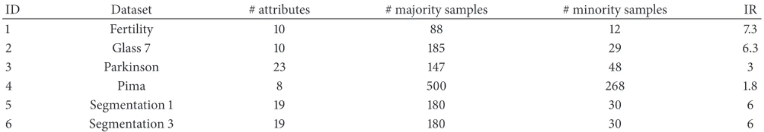
3.1. Experimental Settings and Metrics. Datasets for experi-ments are chosen from UCI machine learning repository [38] and most of them are quite imbalanced. Here we only cope with binary classification problems, so one class is labeled as the minority while the rest merge as the majority in multiclass cases which is similar to other researchers’ preprocess [25, 39, 40]. Table 2 shows the detailed information about the dataset including sample capacity, the number of attributes, the numbers of the minority samples and majority samples, and the imbalance ratio. The imbalance ratio is defined as the result of the cardinality of the majority dividing the cardina-lity of the minority, which may severely influence the perfor-mance of classifiers.

Traditional ensemble methods like AdaBoostM1 and ran-dom forest are chosen for comparison as well. Further illus-tration that should be noticed is that both AdaBoostM1 and random forest can be considered as techniques relieving the imbalance due to the weight-adjustment mechanism by error in AdaBoostM1 and out-of-bag performance monitored in

(6)

Table 2: The basic information about six datasets.

ID Dataset # attributes # majority samples # minority samples IR

1 Fertility 10 88 12 7.3 2 Glass 7 10 185 29 6.3 3 Parkinson 23 147 48 3 4 Pima 8 500 268 1.8 5 Segmentation 1 19 180 30 6 6 Segmentation 3 19 180 30 6

(1) Input the whole dataset𝐷, the number of SVMs-𝐾, the oversampling ratio for Extrapolation Borderline-SMOTE𝛼%.

(2) Train on the original data set𝐷to fit soft margin SVM by choosing a proper kernel and hyper-parameter𝐶in cross-validation and identify the support vectors SV₀= {𝑥(0)_SV𝑖}belonging to the minority

(3) For𝑡from 1 to𝐾:

(4) Bootstrap on the𝐷∼= 𝐷 \SV₀to obtain the sampling result𝐷∼_𝑡 and𝐷𝑐_𝑡 not sampled in the turn𝑡

(5) Get the union set as𝐷∼_𝑡 ∪SV₀and operate extrapolation borderline-SMOTE with the sampling ratio𝛼% on it.

(6) 𝐷∼_𝑡 ∪SV₀and synthetic samples are united as training data set𝐷_𝑡to obtain soft margin SVM𝑓_𝑡(𝑥)with hyper-parameter𝐶chosen by validating the performance on𝐷𝑐_𝑡.

(7) Output the ensemble of SVMs𝐹(𝑥) =sgn(∑_𝑡𝑓_𝑡(𝑥)) Algorithm 4: BEBS algorithm.

Table 3: Confusion matrix.

Predicted positive Predicted negative

Actual positive TP FN

Actual negative FP TN

random forest. We also validated imbalance effect on original SVM. Some state-of-the-art and commonly used algorithms, including random undersampling, random oversampling, SMOTE, and SMOTE-ENN [41] were performed on the above-mentioned dataset as well, all of which would demon-strate the effectiveness of the novel proposed algorithm. Besides, random undersampling, random oversampling, SMOTE, and SMOTE-ENN were combined with SVM for further classification.

In problems of binary classification, confusion matrix offers an intuitive measure for evaluating classifier’s perfor-mance. As illustrated in Table 3, FN is the number of samples identified as negative ones by mistake and the rest can be understood similarly.

The accuracy of the classifier is defined as

Acc= TP+TN

TP+FN+FP+TN. (5) For the problem of IDL, the accuracy is not persuasive for evaluation as depicted before. One of the most frequently used evaluation criteria for IDL is G-means which penalizes

the biased model strictly. G-means is an index averaging geometrically the recall ratios of two classes.

GM= ( TP TP+FN∗ TN FP+TN) 1/2 . (6)

It is obvious that only when both of the recall ratios stay at higher level can the G-means receives better value. So the G-means can be considered to be the trade-off between the accuracy and the recall ratio.

Another evaluation index penalizing the imbalanced effect is𝐹-score defined as

𝐹_𝛽= (1 + 𝛽

2_{) ((}_TP_{/ (}_TP₊_FP_{)) ∗ (}_TP_{/ (}_TP₊_FN₎₎₎

(𝛽2_TP_{/ (}_TP₊_FP_{)) + (}_TP_{/ (}_TP₊_FN₎₎ . (7)

Harmonic average is applied in the index and the param-eter𝛽controls the extent for penalization. Here𝛽is selected as 1.

𝐹-score shows similar performance and shares consis-tency with G-means in our experimental findings, but it averages the precision and recall ratio of one class in essence. Besides, the precision of the minority in one classifier also plays a crucial role in IDL and most of cases show its signi-ficance just as the introduction has described. So the precision was taken into consideration during evaluating process. The precision for the positive is denoted as

Precision= TP

(7)

Table 4: The average results on various dataset using algorithms. ROS means random oversampling while RUS is random undersampling. SMEN is SMOTE-ENN. RF is random forest and ADA is AdaBoostM1.

BEBS SMOTE ROS RUS SMEN SVM RF ADA

Fertility G-means 0.613 0.521 0.446 0.532 0.532 0 0.063 0.424 F-scores 0.285 0.233 0.194 0.23 0.242 0 0.029 0.202 Precision 0.624 0.159 0.128 0.145 0.171 0 0.05 0.194 Glass 7 G-means 0.923 0.912 0.902 0.906 0.891 0.873 0.914 0.906 F-scores 0.736 0.882 0.878 0.845 0.877 0.857 0.876 0.835 Precision 0.902 0.906 0.932 0.842 0.914 0.96 0.914 0.831 Parkinson G-means 0.792 0.523 0.464 0.392 0.436 0.278 0.791 0.776 F-scores 0.63 0.442 0.324 0.284 0.336 0.15 0.729 0.681 Precision 0.671 0.727 0.692 0.278 0.735 0.769 0.809 0.736 Pima G-means 0.753 0.071 0 0 0 0 0.642 0.685 F-scores 0.681 0.011 0 0.02 0 0 0.55 0.613 Precision 0.72 0.654 0 0.07 0 0 0.666 0.632 Segmentation 1 G-means 0.856 0.297 0 0.103 0.262 0 0.873 0.921 F-scores 0.552 0.143 0 0.024 0.144 0 0.85 0.87 Precision 0.731 0.871 0 0.143 0.869 0 0.95 0.85 Segmentation 3 G-means 0.884 0.261 0 0.072 0.193 0 0.746 0.833 F-scores 0.611 0.16 0 0.021 0.094 0 0.665 0.762 Precision 0.792 0.767 0 0.143 0.667 0 0.825 0.841

To obtain a robust result for evaluation, we picked up risk minimization as the criteria in which the minimum metrics of binary class were defined as the corresponding result. Taking precision for an instance, though precisions of both classes can be computed during testing process, the smaller one was selected, just as follows:

Precisionflmin

𝑖 Precision(class𝑖) . (9)

3.2. Results Analysis

3.2.1. Performance Analysis. We, respectively, averaged the results of G-means,𝐹1-score, and precision in 10 independent turns. Table 4 was the final results on various dataset and the top 3 ones in each line were labeled with bold. A direct conclusion drawn from the table was BEBS, random forest, and AdaBoostM1 located in dominating board most of time and behaving stably in three metrics. Some reason accounting for this was that the requirements of careful adaptation about parameters for all the other sampling algorithms seemed crucial. However, the original SVM received worse results on dataset of Fertility, Pima, Segmentation 1, Segmentation 3, and𝐹1-score in Parkinson was rather low. Such phenomenon verified the explanation about skew of SVM in imbalanced case. It was evident that random oversampling, random undersampling, and SMOTE-ENN were sensitive to the datasets because all of them needed parameters of manual setting according to specific case rather than adapting auto-matically. SMOTE outperformed these three methods but was less efficient than our proposed BEBS. Obviously, BEBS which performed well in three metrics stably benefited from both the intuitive extrapolation-SMOTE method involving boundary information and randomness from bootstrapping

technique. To offer a more direct cognition, we ranked the performance of methods on testing sets in decreasing order from the perspective of G-means, 𝐹1-score, and precision. The average ranks of all algorithms on 6 datasets were shown in Figure 4. Also, taking generalization and performance into consideration, random forest and AdaBoostM1 were still worthwhile to make a trial with no additional information.

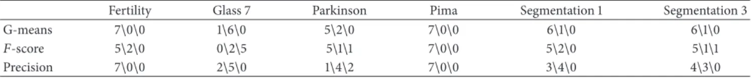
Specifically, with the help of SPSS [42], we carried out Stu-dent’s paired𝑡-test, in which confidence interval of difference was set as 95%, to check the significance of the 10 independent results in comparison. 10 independent results were compared in the form of BEBS versus some other algorithm. Since seven models were chosen for comparison, seven statistical testing results were obtained on each dataset. We looped such process in metrics G-means,𝐹-scores, and precision on each dataset. Furthermore, the seven pairs of the testing have three possible results, respectively, significantly weaker than BEBS and tie, significantly stronger than BEBS. Precise explanation about the result of tie is when the average of 10 independent results in some metrics on the dataset using model 𝐴 is higher or lower than the BEBS but is not significant from the analysis of pair𝑡-test, we directly attribute the reason behind difference to the randomness rather than the mechanism of models and label the paired comparison as tie. The label win means our BEBS’s average of results not only outperforms the comparison model but also passes the hypothesis test. The same is the loss. Combined with Table 4, the results of significance testing were finally mapped into the 3-element tuple in the form of win\tie\loss. Then we counted the frequencies for win, tie, and loss in 7-paired comparison. So the computational results were arranged in the Table 5.

From Table 5, some obvious conclusions were drawn as follows. From the perspective of G-means, about 76.2%

(8)

7.7 5.3 3.5 4 4 1.8 6 6 Rank-G-means BEBS SMO T E RO S RU S SMEN SVM RF AD A 0 2 4 6 8 10 (a) 5.8 _5.3 3.5 _3.2 4.8 2.3 5.8 6 Rank-F1 score BEBS SMO T E RO S RU S SMEN SVM RF AD A 0 1 2 3 4 5 6 7 (b) 5.2 5.2 3.5 2.4 5 4 6.3 5.3 Rank-precision BEBS SMO T E RO S RU S SMEN SVM RF AD A 0 2 4 6 8 (c)

Figure 4: The average rankings of different algorithms on six datasets from three aspects. Rankings are integer scores as 8, 7, 6, 5, 4, 3, 2, and 1 assigned to each algorithm according to the performance.

Table 5: Win\tie\loss counts on results of paired𝑡-test.

Fertility Glass 7 Parkinson Pima Segmentation 1 Segmentation 3

G-means 7\0\0 1\6\0 5\2\0 7\0\0 6\1\0 6\1\0

𝐹-score 5\2\0 0\2\5 5\1\1 7\0\0 5\2\0 5\1\1

Precision 7\0\0 2\5\0 1\4\2 7\0\0 3\4\0 4\3\0

comparison results shown BEBS significantly outperformed other models which was computed as the total number of paired comparisons 42 divided by the number of win counts on the whole dataset 32. The ratio of no loss to others in𝐹 -scores occupied approximately 83.3% and at the same time 64.3% proportion of the total number of paired comparisons indicated superior results using BEBS compared with others significantly. For the precision, only 4.8% of the total counts were significantly poorer than some other models though the proportion of the tie counts maintained about 38.1%. In all, BEBS produced better results after a series of experiments and statistical testing process. The next part would do some research on the stability of the BEBS and some sensitivity analysis experiments were carried out.

3.2.2. Sensitivity Analysis. It is noticed that our proposed algorithm BEBS contains two crucial hyperparameters to

tune, that is, the number of metaclassifiers𝐾and the over-sampling ratio for Extrapolation Borderline-SMOTE𝛼%. Regardless of variations on dataset in the former experiments, the hyperparameters were consistently set as the fixed values 𝐾 = 100and sampling ratio = 0.5. The performance ought to be influenced when such parameters are violated. To investi-gate the robustness of the BEBS, we performed BEBS on the prepared dataset given a tunable range of hyperparameters. As suggested before, G-means is capable of well character-izing the fair results by imposing the penalization on the imbalance consequence. Here sensitivity analysis towards two hyperparameters was carried out and G-means was the objective we concentrated on.

With the sampling ratio fixed as 0.5, we ranged the number of metaclassifiers𝐾 in the interval[70, 130]at the step length 10 and averaged the 10 independent results corre-sponding to the fixed parameters. As Figure 5 illustrated, the six polylines run steadily as𝐾increased and the maximum

(9)

70 80 90 100 110 120 130 Fertility 0.55 0.59 0.57 0.61 0.66 0.7 0.64 Glass 7 0.85 0.93 0.95 0.92 0.94 0.91 0.89 Parkinson 0.74 0.76 0.83 0.79 0.8 0.81 0.77 Pima 0.7 0.76 0.73 0.75 0.74 0.77 0.75 Segmentation 1 0.79 0.88 0.86 0.85 0.82 0.84 0.85 Segmentation 3 Fertility Glass 7 Parkinson Pima Segmentation 1 Segmentation 3 0.85 0.87 0.83 0.88 0.86 0.82 0.89 Number of metaclassifiers K Sensitivity to number of metaclassifiers

0.4 0.5 0.6 0.7 0.8 0.9 1 Va lu e

Figure 5: Sensitivity analysis on the number of metaclassifiers. The value in the table (except the first row) is the averaged results.

Fertility Glass 7 Parkinson Pima Segmentation 1 Segmentation 3 0.3 0.4 0.5 0.6 0.7 Fertility 0.44 0.49 0.61 0.67 0.72 Glass 7 0.77 0.82 0.92 0.96 0.91 Parkinson 0.71 0.77 0.79 0.76 0.6 Pima 0.74 0.76 0.75 0.69 0.62 Segmentation 1 0.82 0.86 0.85 0.87 0.88 Segmentation 3 0.8 0.82 0.88 0.86 0.89 Sampling ratio Sensitivity to sampling ratio

0.4 0.5 0.6 0.7 0.8 0.9 1 Va lu e

Figure 6: Sensitivity analysis on the sampling ratio. The value in the table (except the first row) is the averaged results.

of ranges of G-means values on six polylines was not larger than 0.15. The results suggested BEBS was not sensitive to the number of metaclassifiers at the range[70, 130].

Furthermore, we adapted the sampling ratio in a range of [0.3, 0.7]at the step length 0.1 on the dataset while the number

of metaclassifiers𝐾was maintained as 100. The experimental results were shown in Figure 6. The points on polylines were acquired by averaging G-means values from 10 independent results given a set of parameters as well. An interesting fact lied in the fact that tendencies on Fertility, Glass 7, and

(10)

Segmentation 3 were significant and performance was steadily enhanced when increasing the sampling ratio. The phenomenon may be attributed to the imbalance ratio of dataset. The imbalance ratios on these were not less than 6 from statistical information in Table 2. More synthetic minor-ity samples tended to make contributions towards detecting the actual boundary. So a conclusion can be drawn that when the imbalance ratio retains a rather higher level, the sampling ratio should also adapt to relieve the overfitting circumstance. Results on Parkinson and Pima indicated declines when sam-pling ratio is higher than some thresholds, so higher samsam-pling ratio on not extremely imbalanced dataset may do damage to the final performance. In total, BEBS seems sensitive to the Resampling Ratio and the imbalance ratio should be involved in a fine choice for the parameter.

4. Conclusions

In this paper, a novel ensemble method called BEBS was pro-posed for dealing with the IDL in binary case. The BEBS was framed by employing an adaptive sampling method Extrapo-lation Borderline-SMOTE and bootstrapping aggregation to the former imbalanced dataset. Such variant of SMOTE takes advantage of boundary information derived from the initial SVM and bagging’s mechanism contributes to the relief of overfitting and promotes the capability of model’s general-ization. The decision boundary’s skew towards the minority when using SVM can be revised with the help of synthetic samples. In our experiments, the results on each dataset run for ten times independently to ensure the effectiveness of hypothesis test and further statistical records show BEBS can significantly outperform some representative IDL algorithms in most of time. The sensitivity analysis illustrates the relation between scale of ensemble, sampling ratio, and performance, suggesting BEBS would be extensively enhanced after a proper adaptation according to imbalance ratio of dataset. Future research will summarize general relations between algorithms performance and other attributes like attributes’ number and samples’ cardinality. Multiclass imbalance cases [43] are also considered in the later mining tasks.

Competing Interests

The authors declare that there is no conflict of interests regarding the publication of this paper.

References

[1] H. He and E. A. Garcia, “Learning from imbalanced data,”IEEE Transactions on Knowledge and Data Engineering, vol. 21, no. 9, pp. 1263–1284, 2009.

[2] A. Estabrooks, T. Jo, and N. Japkowicz, “A multiple resampling method for learning from imbalanced data sets,”Computational Intelligence, vol. 20, no. 1, pp. 18–36, 2004.

[3] H. Han, W.-Y. Wang, and B.-H. Mao, “Borderline-SMOTE: a new over-sampling method in imbalanced data sets learning,” in Advances in Intelligent Computing, pp. 878–887, Springer, 2005.

[4] N. V. Chawla, N. Japkowicz, and A. Kotcz, “Editorial: special issue on learning from imbalanced data sets,”ACM SIGKDD Explorations Newsletter, vol. 6, no. 1, pp. 1–6, 2004.

[5] U. Bhowan, M. Johnston, and M. Zhang, “Developing new fitness functions in genetic programming for classification with unbalanced data,” IEEE Transactions on Systems, Man, and Cybernetics, Part B: Cybernetics, vol. 42, no. 2, pp. 406–421, 2012. [6] J.-H. Xue and P. Hall, “Why does rebalancing class-unbalanced data improve AUC for linear discriminant analysis?” IEEE Transactions on Pattern Analysis and Machine Intelligence, vol. 37, no. 5, pp. 1109–1112, 2015.

[7] R. Batuwita and V. Palade, “Class imbalance learning methods for support vector machines,” inImbalanced Learning: Foun-dations, Algorithms, and Applications, pp. 83–99, John Wiley & Sons, Berlin, Germany, 2013.

[8] V. L´opez, A. Fern´andez, S. Garc´ıa, V. Palade, and F. Herrera, “An insight into classification with imbalanced data: empirical results and current trends on using data intrinsic characteris-tics,”Information Sciences, vol. 250, pp. 113–141, 2013.

[9] F. Provost, “Machine learning from imbalanced data sets 101,” inProceedings of the AAAI’2000 Workshop on Imbalanced Data Sets, pp. 1–3, 2000.

[10] L. Pelayo and S. Dick, “Applying novel resampling strategies to software defect prediction,” inProceedings of the Annual Meeting of the North American Fuzzy Information Processing Society (NAFIPS ’07), pp. 69–72, June 2007.

[11] J. Long, J.-P. Yin, E. Zhu, and W.-T. Zhao, “A novel active cost-sensitive learning method for intrusion detection,” in Proceed-ings of the 7th International Conference on Machine Learning and Cybernetics (ICMLC ’08), pp. 1099–1104, IEEE, Kunming, China, July 2008.

[12] K. Zahirnia, M. Teimouri, R. Rahmani, and A. Salaq, “Diagnosis of type 2 diabetes using cost-sensitive learning,” inProceedings of the 5th International Conference on Computer and Knowledge Engineering (ICCKE ’15), pp. 158–163, October 2015.

[13] M. Kubat, R. C. Holte, and S. Matwin, “Machine learning for the detection of oil spills in satellite radar images,”Machine Learn-ing, vol. 30, no. 2-3, pp. 195–215, 1998.

[14] T. Fawcett and F. Provost, “Adaptive fraud detection,” Data Mining and Knowledge Discovery, vol. 1, no. 3, pp. 291–316, 1997. [15] I. Triguero, S. del R´ıo, V. L´opez, J. Bacardit, J. M. Ben´ıtez, and F. Herrera, “ROSEFW-RF: the winner algorithm for the ECBDL’14 big data competition: an extremely imbalanced big data bioinformatics problem,”Knowledge-Based Systems, vol. 87, pp. 69–79, 2015.

[16] Y. Freund and R. E. Schapire, “A decision-theoretic generaliza-tion of on-line learning and an applicageneraliza-tion to boosting,”Lecture Notes in Computer Science (including subseries Lecture Notes in Artificial Intelligence and Lecture Notes in Bioinformatics), vol. 904, pp. 23–37, 1995.

[17] W. Fan, S. J. Stolfo, J. Zhang, and P. K. Chan, “AdaCost: mis-classification cost-sensitive boosting,” inProceedings of the 16th International Conference on Machine Learning (ICML ’99), pp. 97–105, Bled, Slovenia, 1999.

[18] H. Masnadi-Shirazi and N. Vasconcelos, “Cost-sensitive boost-ing,”IEEE Transactions on Pattern Analysis and Machine Intel-ligence, vol. 33, no. 2, pp. 294–309, 2011.

[19] N. V. Chawla, K. W. Bowyer, L. O. Hall, and W. P. Kegelmeyer, “SMOTE: synthetic minority over-sampling technique,”Journal of Artificial Intelligence Research, vol. 16, pp. 321–357, 2002.

(11)

[20] T. Jo and N. Japkowicz, “Class imbalances versus small dis-juncts,”ACM SIGKDD Explorations Newsletter, vol. 6, no. 1, pp. 40–49, 2004.

[21] N. V. Chawla, A. Lazarevic, L. O. Hall, and K. W. Bowyer, “SMOTEBoost: improving prediction of the minority class in boosting,” inKnowledge Discovery in Databases: PKDD 2003: 7th European Conference on Principles and Practice of Knowledge Discovery in Databases, Cavtat-Dubrovnik, Croatia, September 22–26, 2003. Proceedings, vol. 2838, pp. 107–119, Springer, Berlin, Germany, 2003.

[22] G. Wu and E. Y. Chang, “KBA: kernel boundary alignment considering imbalanced data distribution,”IEEE Transactions on Knowledge & Data Engineering, vol. 17, no. 6, pp. 786–795, 2005.

[23] S. Maldonado, R. Weber, and F. Famili, “Feature selection for high-dimensional class-imbalanced data sets using Support Vector Machines,”Information Sciences, vol. 286, pp. 228–246, 2014.

[24] M. Liu, L. Miao, and D. Zhang, “Two-stage cost-sensitive learn-ing for software defect prediction,”IEEE Transactions on Relia-bility, vol. 63, no. 2, pp. 676–686, 2014.

[25] Z. Sun, Q. Song, X. Zhu, H. Sun, B. Xu, and Y. Zhou, “A novel ensemble method for classifying imbalanced data,” Pattern Recognition, vol. 48, no. 5, pp. 1623–1637, 2015.

[26] X.-Y. Liu, J. Wu, and Z.-H. Zhou, “Exploratory undersampling for class-imbalance learning,”IEEE Transactions on Systems, Man, and Cybernetics, Part B: Cybernetics, vol. 39, no. 2, pp. 539– 550, 2009.

[27] R. Batuwita and V. Palade, “Efficient resampling methods for training support vector machines with imbalanced datasets,” in

Proceedings of the 6th IEEE World Congress on Computational Intelligence (WCCI ’10)— International Joint Conference on Neural Networks (IJCNN ’10), Barcelona, Spain, July 2010. [28] G. Wu and E. Y. Chang, “Class-boundary alignment for

imbal-anced dataset learning,” in Proceedings of the International Conference on Machine Learning Workshop on Learning From Imbalanced Data Sets II (ICML ’2003), pp. 49–56, Washington, DC, USA, 2003.

[29] M. Galar, A. Fernandez, E. Barrenechea, H. Bustince, and F. Herrera, “A review on ensembles for the class imbalance prob-lem: bagging-, boosting-, and hybrid-based approaches,”IEEE Transactions on Systems, Man, and Cybernetics, Part C: Applica-tions and Reviews, vol. 42, no. 4, pp. 463–484, 2012.

[30] M. Galar, A. Fern´andez, E. Barrenechea, and F. Herrera, “EUS-Boost: enhancing ensembles for highly imbalanced data-sets by evolutionary undersampling,”Pattern Recognition, vol. 46, no. 12, pp. 3460–3471, 2013.

[31] B. Krawczyk, M. Galar, Ł. Jele´n, and F. Herrera, “Evolutionary undersampling boosting for imbalanced classification of breast cancer malignancy,”Applied Soft Computing Journal, vol. 38, pp. 714–726, 2016.

[32] X. Shi, G. Xu, F. Shen, and J. Zhao, “Solving the data imbalance problem of P300 detection via random under-sampling bagging SVMs,” inProceedings of the International Joint Conference on Neural Networks (IJCNN ’15), July 2015.

[33] V. N. Vapnik,Statistical Learning Theory, Adaptive and Learning Systems for Signal Processing, Communications, and Control, John Wiley & Sons, New York, NY, USA, 1998.

[34] F. Rosenblatt, “The perceptron: a probabilistic model for infor-mation storage and organization in the brain,” Psychological Review, vol. 65, no. 6, pp. 386–408, 1958.

[35] S. Boyd and L. Vandenberghe,Convex Optimization, Cambridge University Press, 2004.

[36] Z.-H. Zhou,Ensemble Methods: Foundations and Algorithms, CRC Press, 2012.

[37] A. Liaw and M. Wiener, “Classification and regression by ran-domForest,”R News, vol. 2, no. 3, pp. 18–22, 2002.

[38] C. Blake and C. J. Merz,UCI Repository of Machine Learning Databases, 1998.

[39] M. Zięba and J. M. Tomczak, “Boosted SVM with active learning strategy for imbalanced data,”Soft Computing, vol. 19, no. 12, pp. 3357–3368, 2015.

[40] Y. Xu, Z. Yang, Y. Zhang, X. Pan, and L. Wang, “A maximum margin and minimum volume hyper-spheres machine with pinball loss for imbalanced data classification,” Knowledge-Based Systems, vol. 95, pp. 75–85, 2016.

[41] G. E. Batista, R. C. Prati, and M. C. Monard, “A study of the behavior of several methods for balancing machine learning training data,”ACM SIGKDD Explorations Newsletter, vol. 6, no. 1, pp. 20–29, 2004.

[42] M. J. Noruˇsis,SPSS/PC+ for the IBM PC/XT/AT, SPSS, 1986. [43] Z. Zhang, B. Krawczyk, S. Garc`ıa, A. Rosales-P´erez, and F.

Herrera, “Empowering one-vs-one decomposition with ensem-ble learning for multi-class imbalanced data,”Knowledge-Based Systems, vol. 106, pp. 251–263, 2016.

(12)

Submit your manuscripts at

https://www.hindawi.com

Computer Games Technology International Journal of

Hindawi Publishing Corporation

http://www.hindawi.com Volume 2014

http://www.hindawi.com Volume 2014 Distributed Sensor Networks International Journal of Advances in

Fuzzy

Systems

International Journal of

Reconfigurable Computing

Applied

Computational

Intelligence and Soft

Computing

Advances in

Artificial

Intelligence

Hindawi Publishing Corporation http://www.hindawi.com Volume 2014 Advances in Software Engineering

http://www.hindawi.com Volume 2014 Electrical and Computer Engineering

Journal of

Computer Networks and Communications

Hindawi Publishing Corporation

http://www.hindawi.com Volume 2014

Multimedia

International Journal of

Biomedical Imaging

Artificial

Neural Systems

Advances in

Robotics

Journal of

http://www.hindawi.com Volume 2014 Hindawi Publishing Corporationhttp://www.hindawi.com Volume 2014

Computational Intelligence and Neuroscience

Modelling & Simulation in Engineering

The Scientific

World Journal

Human-Computer Interaction

Advances in

Computer EngineeringAdvances in