MINING TIME SERIES DATA BASED UPON CLOUD MODEL
Hehua Chi a, Juebo Wu b, *, Shuliang Wang a, b, Lianhua Chi c, Meng Fang a
a
International School of Software, Wuhan University, Wuhan 430079, China - [email protected]
bState Key Laboratory of Information Engineering in Surveying, Mapping and Remote Sensing, Wuhan University,
Wuhan 430079, China - [email protected]
c
School of Computer Science and Technology, Huazhong University of Science and Technology, Wuhan 430074,
China – [email protected]
KEY WORDS: Spatial Data Mining, Time-series, Cloud Model, Prediction
ABSTRACT:
In recent years many attempts have been made to index, cluster, classify and mine prediction rules from increasing massive sources of spatial time-series data. In this paper, a novel approach of mining time-series data is proposed based on cloud model, which described by numerical characteristics. Firstly, the cloud model theory is introduced into the time series data mining. Time-series data can be described by the three numerical characteristics as their features: expectation, entropy and hyper-entropy. Secondly, the features of time-series data can be generated through the backward cloud generator and regarded as time-series numerical characteristics based on cloud model. In accordance with such numerical characteristics as sample sets, the prediction rules are obtained by curve fitting. Thirdly, the model of mining time-series data is presented, mainly including the numerical characteristics and prediction rule mining. Lastly, a case study is carried out for the prediction of satellite image. The results show that the model is feasible and can be easily applied to other forecasting.
* Corresponding author. [email protected].
1. INTRODUCTION
With the rapid development of spatial information technology, especially spatial data acquisition technology, spatial database has become the data basis of many applications. Through the spatial data mining or knowledge discovery, we can obtain the general knowledge of geometry from spatial databases, including spatial distribution, spatial association rules, spatial clustering rules and spatial evolution rules, which can provide a powerful weapon for making full use of spatial data resources [1, 2]. As in the real world, most of the spatial data is associated with the time; more and more researchers have started to pay attention to the time series data mining. Time series model mining plays an important role in data mining.
Time series forecasting has always been a hot issue in many scientific fields. The study of time series data includes the following important aspects: trend analysis, similarity search, sequential pattern mining and cycle pattern mining of time-related data, time series prediction and so on. G. Box et al. divided the sequence into several sub-sequences through a moving window, and then discovered characteristic change pattern following the way of association rules by making use of clustering to classify these sub-sequences as a specific pattern of change [3]. J. Han et al. used the data mining technology to study cycle fragments and part of cycle fragments of the time series in the time series database, in order to discover the cyclical pattern of time series [4]. In the research [5], the authors proposed cyclic association rule mining. The literature [6] proposed calendar association rule mining. R. Agrawal et al. had given a series of sub-sequence matching criterion [7]. Two sequences were considered similar when existing a sufficient number of non-overlapping and similar sub-sequences timing right between them. Since the literature [8] published the first research paper about piecewise linear fitting algorithm for
sequence data, relevant research has received extensive attention [9, 10, 11]. This simple and intuitive linear fitting representation used a series of head and tail attached linear approximation to represent time series. In combination with cloud model, W. H. Cui et al. proposed a new method of image segmentation based on cloud model theory to add uncertainty of image to the segmentation algorithm [12]. X. Y. Tang et al. presented a cloud mapping space based on gradation by the cloud theory aiming to solve the problem of land use classification of RS image [13]. K. Qin proposed a novel way for weather classification based on cloud model and hierarchical clustering [14]. In applications, time series analysis has been widely used in various fields of society, such as: macro-control of the national economy, regional integrated development planning, business management, market potential prediction, weather forecasting, hydrological forecasting, earthquake precursors prediction, environmental pollution control, ecological balance, marine survey and so on.
The time series mining research has received some progress, but there are still some shortcomings. For example: time series should be smooth and normal distribution. This paper presents a prediction model based on cloud model. This model describes the features of time series data through three numerical characteristics. The time series data, such as images, are standardized as the cloud droplets after the pre-processing, and then are executed cloud transform through backward cloud generator to get three numerical characteristics. Similarly, we can calculate number of sample data sets to obtain a series of cloud numerical characteristics. Through curve fitting, we can mine the prediction rules to achieve data prediction.
2. THE CLOUD MODEL 2.1 The cloud model
Cloud model is proposed by D. Y. Li in 1996 [15]. As the uncertainty knowledge of qualitative and quantitative conversion of the mathematical model, the fuzziness and randomness fully integrated together, constituting a qualitative and quantitative mapping.
Definition: Let U be a universal set described by precise numbers, and C be the qualitative concept related to U. Assume that there is a number x∈U that randomly stands for the concept C and the certainty degree of x for C, which is a random value with stabilization tendency and meets:
μ : U→[0,1] x ∈ U x →μ(x)
where the distribution of x on U is defined as cloud land. Each x is defined as a cloud drop. Figure 1 shows the numerical characteristics {Ex En He} of the cloud.
Figure 1. The numerical characteristics {Ex En He} In the cloud model, we employ the expected value Ex, the entropy En, and the hyper-entropy He to represent the concept as a whole.
The expected value Ex: The mathematical expectation of the cloud drop distributed in the universal set.
The entropy En: The uncertainty measurement of the qualitative concept. It is determined by both the randomness and the fuzziness of the concept.
The hyper-entropy He: It is the uncertainty measurement of the entropy, i.e., the second-order entropy of the entropy, which is determined by both the randomness and fuzziness of the entropy.
2.2 Backward cloud generator
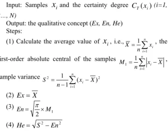
Backward cloud generator is uncertainty conversion model which realizes the random conversion between the numerical value and the language value at any time as the mapping from quantitative to qualitative. It effectively converts a certain number of precise data to an appropriate qualitative language value (Ex, En, He). According to that, we can get the whole of the cloud droplets. The more the number of the accurate data is, the more precise the concept will be. Through the forward and reverse cloud generator, cloud model establishes the interrelated
and interdependent relations. The algorithm of backward cloud generator is as follows:
Input: Samples and the certainty degree (i=1, 2…, N)
i
x
CT(xi)Output: the qualitative concept (Ex, En, He) Steps:
(1) Calculate the average value of
x
i, i.e.,∑
= = n i i x n X 1 1 , the first-order absolute central of the samples∑
= Ι= − n i i X x n M 1 1 , sample variance
∑
= − − = n i i X x n S 1 2 2 ( ) 1 1 (2) Ex=X (3) Ι × = M En 2 π (4) 2 2 En S He= −3. TIME-SERIES MINING MODEL BASED ON CLOUD MODEL
Using cloud model theory, this section proposes the framework of series data mining, and gives concrete steps. The time-series data can be described by the three numerical characteristics of cloud model.
3.1 Time-series data mining framework based on cloud model
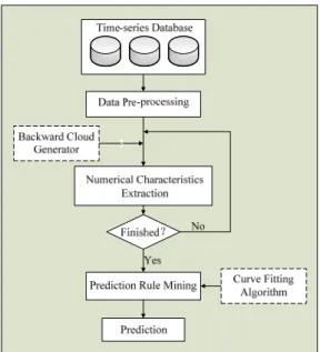
The main idea of time-series data mining framework based on cloud model is as follows:
Firstly, extract the experimental data from the time-series databases and pre-process the data to obtain cloud droplets. Secondly, make use of backward cloud generator algorithm to extract the numerical characteristics {Ex En He} of the cloud droplet.
Thirdly, extract the numerical characteristics {Ex En He} of the each cloud droplet and get all groups of the numerical characteristics {Ex En He}.
Finally, make use of the fitting algorithm to do the fitting of all groups of the numerical characteristics {Ex En He}, in order to achieve forecast according to the curve.
The framework of time-series data mining and the main flow based on cloud model are shown in Figure 2, where gives the specific description of this framework.
3.2 Data pre-processing
The main purpose of data pre-processing is to eliminate irrelevant information and to recovery useful information. The time-series data from time-series database is rough, and it is necessary to pre-process data in order to carry out the next step. The object of cloud model is cloud droplets. We have to turn the time-series data into cloud droplets as the input of the cloud model.
Figure 2. The framework of time-series data mining based on cloud model
3.3 Numerical Characteristic Extraction
Through the numerical characteristic extraction of the time-series data based on cloud model, we can obtain the numerical characteristics sets of time-series data. These characteristics are direct descriptions of the time-series data on behalf of the internal information. Time-series data can come from time-series database and can also change over time. We can also make use of backward cloud generator to extract numerical characteristics. The algorithm is referred as section 2.2.
The numerical characteristics {Ex En He} of the cloud reflect the quantitative characteristics of the qualitative concept. Ex (Expected value): The point value, which is the most qualitative concept in the domain space, reflects the cloud gravity centre of the concept.
En (Entropy): Entropy is used to measure the fuzziness and
probability of the qualitative concept, reflecting the uncertainty of qualitative concept. The entropy of time-series data can reflect the size range of the cloud droplet in the domain space. He (Hyper entropy): The uncertainty of the entropy-entropy's entropy reflects the cohesion of all the cloud droplets in the domain space. The value of the hyper entropy indirectly expresses the dispersion of the cloud.
By the numerical characteristic extraction of the time-series data based on cloud mode, we can get the numerical characteristics of a large number of cloud droplets. These numerical characteristics extracted from the time-series data describe the overall features, as well as the trend of development and change over time. The next step is the curve fitting of the numerical characteristics to obtain prediction rules.
3.4 Prediction Rule Mining
The process is mainly to identify the prediction curves. We regard the numerical characteristic extraction of the time-series data based on cloud model as the sample set of a curve fitting, and get the fitting curve by the curve-fitting method. Due to the differences of the time-series data, we should choose the proper
curve-fitting algorithm in the specific application. For example, by using the least square method. The (Ex En He) of time-series data is effectively fitted to achieve the prediction rule mining. According to causality between prediction objects and factors, we can achieve the prediction. There are many factors associating with the target. We must choose the factors having a strong causal relationship to achieve the prediction. There are two factors variable X and the dependent variable Y to express the prediction target. If they are the linear relationship between X and Y, then the relationship is Y=a+bX. But if they are the nonlinear relationship between X and Y, then the relationship maybe is Y=a+b1X+b2X2+... or others. The a and b in the formula are the agenda coefficients. They can be valued by the statistical or other methods. The time-series for short term prediction is more effective. However, if it is used for long-term prediction, it must also be combined with other methods. After getting the prediction curves, we can carry out the further work, namely, to predict future trends of the time-series data.
3.5 Prediction
The time series is a chronological series of observations. By the previous step, we can get one or more fitting curves. These curves are as predictable rules. By these prediction rules, we can carry out time series data prediction. According to the knowledge of the function and time parameters, we can obtain relationship value of fitting curve function. Making use of function relationship, we can predict and control the problem under the given conditions in order to provide data for decision-making and management. After getting mathematical model of long-term trends, seasonal changes and irregular changes by historical data of time series, we can use them to predict the value T of long-term trends, the value S of seasonal changes and the value I of irregular changes in the possible case. And then we calculate predicted value Y of the future time series by using these following models:
Addition mode T + S + I = Y Multiplicative model T × S × I = Y
If it is hard to get predicted value of irregular changes, we can obtain the predicted value of long-term trends and seasonal changes by putting the multiplier or sum of the above two as predicted value of time series. If the data itself have not seasonal changes or not need to forecast quarterly sub-month data, the predicted value of long-term trends is the predicted value of time series, that is, T = Y. In such way, by predicting the rules curves, we can predict the time series data to discover the laws of development of things and make a good decision-making for us.
4. A CASE STUDY
In order to verify the validity of the time-series data mining based on cloud model, we make an experiment about the satellite images in this section. The experiment makes use of the real-time satellite cloud image from the Chinese meteorological. Through the analysis of historical data, we can obtain the prediction rules to carry out the prediction of weather trends.
4.1 Data acquisition
In this study, data sources come from the satellite cloud data of Chinese meteorological. The website: http://www.nmc.gov.cn/. These data are time dynamic. The satellite makes the real-time photography, and then returns the data to earth. We choose
the three kinds of data as the data source, China and the Western North Pacific Sea Infrared Cloud, China Regional Vapour Cloud, China Regional Infrared Cloud. These data have the following characteristics: Time-series property, synchronization property and consistent view property.
We collect a total of 6 months of the historical data to make the experiments. After data collection, we select the 1600 images of China and the Western North Pacific Sea Infrared Cloud, 1800 images of China Regional Vapour Cloud and 2700 images of China Regional Vapour Cloud, as the sample sets of the experiments. Part of the sample sets are shown in Figure 3, Figure 4 and Figure 5.
Figure 3: China and the Western North Pacific Sea Infrared Cloud
Figure 4: China Regional Vapour Cloud
Figure 5: China Regional Infrared Cloud
⎥ ⎥ ⎥ ⎥ ⎥ ⎥ ⎥ ⎥ ⎦ ⎤ ⎢ ⎢ ⎢ ⎢ ⎢ ⎢ ⎢ ⎢ ⎣ ⎡ ... ... ... ... ... ... ... ... ... 124 121 121 122 125 122 130 ... 124 124 124 125 124 119 132 ... 125 125 127 128 123 116 130 ... 125 125 128 127 119 115 124 ... 123 128 130 124 117 114 125
Figure 6: Pixel matrix
4.2 Data pre-processing
In order to handle easily, it should do pre-processing for satellite cloud images before mining the knowledge. The main purpose is to extract the image pixel value. First, satellite images needs to be transformed to the same size. Then, the images should be converted into grid with extracting the corresponding pixel value. The size of the grid is set depending on image content. Through the above steps, a pixel matrix can be obtained. The value of each matrix can be as a cloud droplet in cloud transformation. Figure 6 shows a satellite image
corresponding to the value of the pixel matrix, that is, cloud droplets.
4.3 Image Feature Extraction
This step is primarily to do satellite imagery feature extraction and get a collection of three numerical characteristics based on cloud model features. Input data are the pixel values obtained from the pre-processing step. Each pixel value corresponds to the backward cloud generator among the cloud droplets. The implementation process can refer to Section 2.2, and the main function is to achieve the following:
Calculate expectation value:
ImageExp=SelectAveImage(Images, Num); Calculate entropy:
ImageEn=CalculateStdImage(Images, ImageExp, Num); Calculate hyper-entropy:
ImageHe=CalculateReVarianceImage(1, ImageEn); The data sets of cloud features of satellite images can be generated in this step, which can be as the data source for prediction curve fitting.
4.4 Curve Fitting Prediction
Through the backward cloud generator, we have a sample set of the numerical characteristics based on cloud model. We can get the curve fitting by the sample sets. In this study, we use the least square curve fitting method. For each type of data, we can get three prediction curves, that is, the expected value curve, the entropy curve and the hyper entropy curve. Main function is: Define the solving functions of the polynomial fitting coefficient; x, y as the input data; n as the numbers of fitting:
function A=nihe(x,y,n) Measure the length of data:
m=length(x); Generate the X matrix:
X1=zeros(1,2*n); … X2=[m,X1(1:n)]; X3=zeros(n,n+1); … X3(j,:)=X1(j:j+n);end X=[X2;X3]; Y=zeros(1,n); … Y=[sum(y),Y];Y=Y'; Obtain fitting coefficient vectors A:
A=X/Y;
4.5 Prediction analysis
Through the above steps and each type of satellite images, we can get three different projection curves. We look them as the prediction rules to forecast the future satellite cloud.
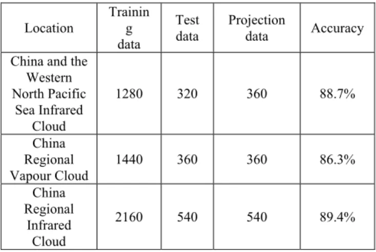
In this study, we use 80% of the sample sets as the training sets and another 20% of the data as the prediction reference value. By comparing the prediction values with actual value, we can get the model prediction accuracy rate. The results are shown in table 1. It shows the results of the different types of satellite
cloud through the prediction model, the average accuracy rate of three kinds of satellite cloud is 88.13% and meets projection demands. The results show that the projection of satellite cloud is feasible. Location Trainin g data Test data Projection data Accuracy China and the
Western North Pacific Sea Infrared Cloud 1280 320 360 88.7% China Regional Vapour Cloud 1440 360 360 86.3% China Regional Infrared Cloud 2160 540 540 89.4%
Table 1: the results of the satellite cloud projection
5. CONCLUSIONS
Most of the spatial data have the time dimension, and will change over time. Time series space contains the time dimension in spatial association characteristics and can get time series space association rules through time series space association rule mining. This paper presented a method of time series data rules mining, which played an important significance for getting time series space association rules and doing the practical application by time series space association rules. First, by the backward cloud generator and the three numerical characteristics of cloud model, this model described the features of time series data. Second, the digital features of a series of sample sets were obtained as the training sample sets. Then, by these feature points, the rule curve fitting was predicted for obtaining predictive models. Finally, the time series data were predicted by the forecasting rules. The experimental results showed that the method is feasible and effective. Through the data standardization processing, this method can be extended to multiple applications. Time series data mining is an interdisciplinary science and the further research including the following aspects:
(1) Other research of curve fitting method.
(2) The combination of research of cloud model and other algorithms.
(3) The visualization studies of time series and time sequence similarity studies.
6. ACKNOWLEDGEMENTS
This paper is supported by National 973 (2006CB701305, 2007CB310804), National Natural Science Fund of China (60743001), Best National Thesis Fund (2005047), and National New Century Excellent Talent Fund (NCET-06-0618).
7. REFERENCES
[1] D. R. Li, S. L. Wang, W. Z. Shi et al. On Spatial Data Mining and Knowledge Discovery [J]. Geomatics and Information Science of Wuhan University, 2001, 26(6): 491-499.
[2] S. Shekhar, P. Zhang, Y. Huang et al. Trends in Spatial Data Mining. In: H.Kargupta, A.Joshi(Eds.), Data Mining: Next Generation Challenges and Future Directions[C]. AAAI/MIT Press, 2003, 357-380.
[3] G. Box, G. M. Jenkins. Time series analysis: Forecasting and control, Holden Day Inc., 1976.
[4] J. Han, G. Dong, Y. Yin. Efficient mining of partial periodic patterns in time series database. In Proc. 1999 Int. Conf. Data Engineering (ICDE'99), pages 106-115, Sydney, Australia, April 1999.
[5] B. Ozden, S. Ramaswamy, A. Silberschatz. Cyclic associ-ation rules. Proceedings of the 15 th Internassoci-ational Conference on Data Engineering. 1998, 412-421.
[6] Y. Li, P. Ning, X. S. Wang et al. Discovering calendar-based temporal association rules. Data&Knowledge Engineer-ing, 2003, 44: 193-218.
[7] R. Agrawal, K. I. Lin, H. S. Sawhney et al. Fast Similarity Search in the Presence of Noise, Scaling, and Translation in Time-Series Databases. Proceedings of the 21th International Conference on Very Large Data Bases, 1995, 490-501.
[8] T. Pavlidis, S. L. Horowitz. Segmentation of plane curves. IEEE Trans. Comput. 23, 1974, 860-870.
[9] S. Park, S. W. Kim, W. W. Chu. Segment-based approach for subsequence searches in sequence databases. In
Proce-edings of the Sixteenth ACM Symposium on Applied
Computing
, 2001, 248-252.[10] K. B. Pratt, E. Fink. Search for patterns in compressed time series. International Journal of Image and Graphics, 2002, 2(1): 89-106.
[11] H. Xiao, Y. F. Hu. Data Mining Based on Segmented Time Warping Distance in Time Series Database [J]. Computer Research and Development, 2005, 42(1): 72-78.
[12] W. H. Cui, Z. Q. Guan, K. Qin. A Multi-Scale Image Segmentation Algorithm Based on the Cloud Model. Proc. 8 th spatial accuracy assest. in natural resources, World Academic Union, 2008.
[13] X. Y. Tang, K. Y. Chen, Y. F. Liu. Land use classification and evaluation of RS image based on cloud model. Edited by Liu, Yaolin; Tang, Xinming. Proceedings of the SPIE, 2009, Vol.7492, 74920N-74920N-8.
[14] K. Qin, M. Xu, Y. Du et al. Cloud Model and Hierarchical Clustering Based Spatial Data Mining Method and Application. The International Archives of the Photogrammetry, Remote Sensing and Spatial Information Sciences. Vol. XXXVII. Part B2, 2008.
[15] D. R. Li, S. L. Wang, D. Y. Li. Spatial Data Mining Theories and Applications. Science Press, 2006.