EJASA, Electron. J. App. Stat. Anal.
http://siba-ese.unisalento.it/index.php/ejasa/index
e-ISSN: 2070-5948
DOI: 10.1285/i20705948v10n2p499
Volatility estimation using support vector ma-chine: Applications to major foreign exchange rates
By Chung, Zhang
Published: 14 October 2017
This work is copyrighted by Universit`a del Salento, and is licensed un-der aCreative Commons Attribuzione - Non commerciale - Non opere derivate 3.0 Italia License.
For more information see:
DOI: 10.1285/i20705948v10n2p499
Volatility estimation using support
vector machine: Applications to major
foreign exchange rates
Steve S. Chung
∗aand Serin Zhang
baDepartment of Mathematics, California State University, Fresno bDepartment of Statistics, Florida State University
Published: 14 October 2017
In finance, volatility is fundamentally important because it is associated with the risk. A growing body of literature shows that risks associated with volatility are priced in stock, option, bond, and foreign exchange markets. Therefore, accurate estimation of the volatility is critical in financial markets. The generalized autoregressive conditional heteroskedasticity (GARCH) has been one of the most popular volatility models and the model parameters are usually estimated from the conditional maximum likelihood estimation (MLE) method. In this paper, we attempt to improve the MLE-based GARCH forecast using the support vector machine (SVM). We also compare the SVM-based volatility model with the two popular asymmetric volatility models: exponential GARCH (E-GARCH) and Glosten-Jagannathan-Runkle GARCH (GJR-GARCH). We carry out the analysis through simulations and real datasets. The results show that the SVM-based volatility models provide better predictive potential than the existing parametric volatility models. Keywords: Volatility; support vector machine; financial time series; GARCH; E-GARCH; GJR-GARCH; foreign exchange rates.
1 Introduction
Volatility modeling has been a very active and extensive research area in empirical finance and time series economics for both academics and practitioners. Pioneer works include
∗
Corresponding author: [email protected].
c
Universit`a del Salento ISSN: 2070-5948
the autoregressive conditional heteroskedasticity (ARCH) of Engle (1982) and the gener-alized autoregressive conditional heteroskedasticity (GARCH) of Bollerslev (1986). The parameters are usually estimated from (conditional) maximum likelihood (ML) proce-dures that are optimal if the data come from a Gaussian distribution. The popularity of ARCH and GARCH processes comes from the fact that they have a simple model specifi-cation and good interpretability. They have been frequently used in the parametrization of conditional heteroskedasticity in the literature, especially, the standard GARCH(1,1) model, which is specified as
σt2=ω+αyt2−1+βσt2−1, (1) whereω, α, andβ are positive values. Gokcan (2000) showed that GARCH(1,1) model outperformed exponential GARCH model when applied to the monthly stock market returns of seven emerging countries. Hansen and Lunde (2005) compared GARCH(1,1) with 330 ARCH-type models and found no evidence that it is outperformed by more sophisticated models. Furthermore, GARCH(1,1) has been used as a benchmark model for more complicated model specifications.
Despite the popularity and wide applicability, the GARCH model suffers from several weaknesses and drawbacks. Nelson (1991) criticized the GARCH model in three aspects: (1) parameters are restricted to be positive at every time point; (2) it fails to accom-modate the asymmetry effect (or leverage effect); and (3) measuring the persistence of the shocks on volatility is difficult. Nelson (1991) proposed the exponential GARCH (E-GARCH), which accommodates the drawbacks of a standard GARCH model. The first-order E-GARCH, or E-GARCH(1,1), process specifies the model as
logσ2t =ω+g(εt−1) +βlog σ2t−1
, (2)
where g(εt−1) =αεt−1+γ(|εt−1| −E|εt−1|). For standard normal random variable εt, E(|εt|) = p 2/π and E(|εt|) = 2√v−2Γ[(v+ 1)/2] (v−1)Γ(v/2)√π
fort-distribution random variable withvdegrees of freedom. Unlike the GARCH model, the E-GARCH model relaxes the positivity restriction by using the logged conditional variance and responds asymmetrically to positive and negative shocks. However, E-GARCH(1,1) with normal errors does not adequately characterize the process with high kurtosis and slowly decaying autocorrelations. One can find more details from Malmsten and Terasvirta (2004).
Another popular volatility model that asymmetrically treats both positive and nega-tive shocks on the volatility is the Glosten-Jagannathan-Runkle GARCH (GJR-GARCH) model of Glosten, Jagannathan, and Runkle (1993). GJR-GARCH(1,1) model is defined as
σt2 =ω+αyt2−1+γIt−1y2t−1+βσ2t−1, (3)
where It is an indicator function taking the values of 1 for yt ≤0 and 0 otherwise and ω, α, γ, and β are positive values. This model is often called the threshold GARCH (T-GARCH) model in the literature. The main feature of this model is that a negative shock
has a larger impact than a positive shock and hence, it captures the leverage effect. Like the GARCH model, the GJR-GARCH model captures the volatility clustering. Also, it can be shown that the unconditional distribution presents excess kurtosis even under the Gaussian distribution.
The aim of this paper is to examine the predictability of volatility using support vector machine (SVM) and compare its performance with aforementioned parametric volatil-ity models: GARCH(1,1), E-GARCH(1,1), and GJR-GARCH(1,1). A few attempts have been made to estimate the volatility using support vector machine, which showed evidence of improved performances. Perez-Cruz et al. (2003) used the support vec-tor machine to estimate the GARCH parameters and compared with that of maximum likelihood estimates. Chen et al. (2010) proposed SVM-based GARCH model and compared with simple moving average, standard GARCH, nonlinear EGARCH and tra-ditional ANN-GARCH models. Ou and Wang (2010) compared the least square support vector machine with the classical GARCH(1,1), E-GARCH(1,1), and GJR-GARCH(1,1) models to forecast the financial volatilities using three major ASEAN stock markets.
The remainder of this paper is organized as follows. Section 2 gives a description of the support vector machine in a regression setting. In Section 3, we conduct the simulation study and report its result and section 4 considers the six major foreign exchange rates as real-data examples. Section 5 concludes.
2 Theory of SVM for Regression
In a support vector machine (SVM), we first consider a training dataset (xt, yt), where
xt ∈ Rp, yt ∈ R1, and t = 1, ..., n. In a context of time series analysis, xt is the set
of lagged values of yt. That is, xt = (yt−1, yt−2, ..., yt−p). We assume that the data are generated from a function
yt=f(xt) +et, (4)
in which f can be approximated by
f(xt) =w0φ(xt) +b, (5)
whereφ(·) is a nonlinear transformation to a higher dimension space. That is,xt ∈Rp 7→ φ(xt)∈Rq forp≤q. Proposed by Vapnik (1995), we consider a linear-insensitive loss function defined by
L= (
|y−f(xt)| −, |y−f(xt)| ≥
0, otherwise.
This loss function does not penalize errors below . It indicates that the training data within the-tube have no loss and do not provide any information for decision. Hence, the function f(xt) is constructed only through those data points located on or outside
the -tube. The computation of SVM is greatly simplified because of this property of sparseness, which results from the -insensitive loss function.
The non-negative slack variables,ξtandξt∗ are introduced to describe the-insensitive loss and the constrained optimization problem is as follows
min w,b,ξi,ξi∗ " 1 2kwk 2+C n X t=1 (ξt+ξt∗) # subject to yt−w0φ(xt)−b≤+ξt (6) w0φ(xt) +b−yt≤+ξt∗ (7) ξt, ξt∗≥0. (8)
The slack variables,ξtandξt∗, deal with the samples with prediction error greater than andC is the penalty parameter. This problem can be solved by introducing constraints (6)-(8) using the Lagrange multipliers that leads to the minimization of
LP = 1 2kwk 2+C n X t=1 (ξt+ξt∗) − n X t=1 αt(+ξt−yt+w0φ(xt) +b)− n X t=1 µtξt − n X t=1 α∗t(+ξt∗+yt−w0φ(xt)−b)− n X t=1 µ∗tξt∗
with respect to w, b, ξt, and ξ∗t and maximization with respect to the Lagrange multi-pliers,αt, α∗t, µt, andµ∗t. By computing Karush-Kunh-Tucker (KKT) (Fletcher (1987)) conditions, we have ∂Lp ∂w =w− n X t=1 (αt−α∗t)φ(xt) = 0, ∂Lp ∂b = n X t=1 (αt−α∗t) = 0, ∂Lp ∂ξt =C−αt−µt= 0, ∂Lp ∂ξ∗t =C−α ∗ t −µ∗t = 0, αt[+ξt−yt+w0φ(xt) +b] = 0, α∗t[+ξt∗−w0φ(xt)−b+yt] = 0, µtξt= 0, and µ∗tξ ∗ t = 0,
whereαt, α∗t, µt, µ∗t ≥0. These conditions lead to the maximization of L= n X t=1 (αt+α∗t)− n X s=1 n X t=1 (αs−αs∗)(αt−α∗t)φ0(xs)φ(xt). (9)
with subject to 0≤αt, α∗t ≤C. Quadratic programming schemes (Sch¨olkopf and Smola (2001)) can be used to solve this problem and, in solving (9), we need to know the reproducing kernel in Hilbert Space (RKHS) κ(xs,xt) = φ0(xs)φ(xt). Some widely
used kernels are
(Linear) κ(xs,xt) =x0sxt, (10) (Polynomial) κ(xs,xt) = (x0sxt+ 1)d, (11) (Radial basis function)κ(xs,xt) =exp(−kxs−xtk2/(2σ2)), (12) whered= 1,2,3, ..., andσ >0. Note that the parameterin (9) can be useful if we can specify the accuracy of the approximation beforehand. However, sinceheavily depends on data, it is very hard to choose a priori a good value, which may make the SVM regression difficult. In our analysis, we usedν-SVM regression, called ν−SVR, to avoid this difficulty, which basically replaces with ν ∈ (0,1). ν represents an approximate proportion of the support vectors and hence, it gives the complexity of the machine. One can refer to Sch¨olkopf and Smola (2001) for more details.
We fix the value of C to be 1 for all simulations and real datasets since the solution is not sensitive to this parameter. The value of ν was determined by the fivefold cross validation. We divided the dataset into five disjoint sets and used four of them to train several machines with different values for ν. The fifth set was to used to compute the validation error of each machine for each specific value of ν. The values that we chose were ν ={0.1,0.2, ...,0.9}. This process was repeated four times. We used the value of ν that gave us the minimum error.
3 Simulation Studies
The aim of this section is to investigate the proposed method through simulations. We assume that the return seriesyt come from a data generating process (DGP)
yt=σtεt, (13)
fort= 1, ..., n. The innovation seriesεt are identical and independent random variables with mean 0 and variance τ2. The mean function can be included and estimated but we do not consider this in our current work. We chose the distributions of εt to be the standard normal and t-distribution with 3 degrees of freedom in our simulations.
The latent variable σt in (13) is called the volatility in finance and it cannot be measured in practice. Following Perez-Cruz et al. (2003), we measure σt2 as a moving average of the four-lagged squared return series. That is,
ˆ σ2t = 1 5 4 X k=0 yt2−k.
Hence, we can estimate the volatility under the GARCH(1,1)-framework given by ˆ
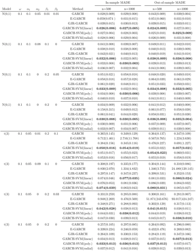
Table 1: Average values of MADE from 50 independent simulations from each model. The standard deviations are in the parentheses.
In-sample MADE Out-of-sample MADE Model ω α1 α2 β1 β2 Method n=500 n=1000 n=500 n=1000 N(0,1) 0.1 0.1 0.05 0.01 0.01 GARCH 0.028(0.009) 0.029(0.008) 0.043(0.009) 0.039(0.004) E-GARCH 0.059(0.074 ) 0.031(0.015) 0.051(0.060) 0.031(0.010) GJR-GARCH 0.039(0.015) 0.030(0.013) 0.039(0.015) 0.033(0.011) GARCH-SVM(linear) 0.026(0.006) 0.027(0.005) 0.024(0.009) 0.027(0.001) GARCH-SVM(poly.) 0.027(0.004) 0.028(0.003) 0.025(0.010) 0.025(0.009) GARCH-SVM(radial) 0.028(0.006) 0.029(0.004) 0.026(0.009) 0.031(0.008) N(0,1) 0.1 0.1 0.08 0.1 0 GARCH 0.041(0.008) 0.039(0.007) 0.049(0.011) 0.042(0.010) E-GARCH 0.038(0.010) 0.038(0.008) 0.040(0.013) 0.039(0.009) GJR-GARCH 0.043(0.021) 0.040(0.013) 0.040(0.019) 0.041(0.018) GARCH-SVM(linear) 0.032(0.006) 0.032(0.005) 0.038(0.009) 0.038(0.008) GARCH-SVM(poly.) 0.033(0.008) 0.030(0.003) 0.039(0.013) 0.039(0.013) GARCH-SVM(radial) 0.036(0.007) 0.032(0.004) 0.041(0.008) 0.039(0.005) N(0,1) 0.1 0.1 0 0.2 0.05 GARCH 0.051(0.021) 0.058(0.018) 0.048(0.020) 0.049(0.018) E-GARCH 0.058(0.018) 0.057(0.028) 0.064(0.039) 0.061(0.029) GJR-GARCH 0.061(0.020) 0.048(0.011) 0.051(0.033) 0.050(0.031) GARCH-SVM(linear) 0.033(0.009) 0.032(0.004) 0.034(0.008) 0.033(0.005) GARCH-SVM(poly.) 0.034(0.008) 0.030(0.006) 0.039(0.008) 0.039(0.007) GARCH-SVM(radial) 0.040(0.010) 0.037(0.010) 0.041(0.011) 0.040(0.009) N(0,1) 0.1 0.1 0 0.2 0 GARCH 0.034(0.009) 0.032(0.006) 0.041(0.012) 0.040(0.008) E-GARCH 0.158(0.315) 0.049(0.012) 0.061(0.077) 0.058(0.038) GJR-GARCH 0.061(0.041) 0.044(0.020) 0.058(0.031) 0.051(0.030) GARCH-SVM(linear) 0.030(0.008) 0.030(0.005) 0.036(0.008) 0.035(0.004) GARCH-SVM(poly.) 0.030(0.009) 0.031(0.006) 0.037(0.009) 0.037(0.007) GARCH-SVM(radial) 0.033(0.007) 0.034(0.007) 0.039(0.011) 0.039(0.008) t(3) 0.1 0.05 0.01 0.2 0.1 GARCH 0.365(0.145) 0.349(0.129) 0.364(0.137) 0.347(0.109) E-GARCH 0.712(1.461) 2.716(11.768) 0.567(0.765) 1.224(3.630) GJR-GARCH 0.384(0.156) 0.345(0.116) 0.476(0.227) 0.691(1.227) GARCH-SVM(linear) 0.050(0.016) 0.054(0.019) 0.055(0.022) 0.057(0.021) GARCH-SVM(poly.) 0.051(0.017) 0.055(0.023) 0.054(0.023) 0.060(0.031) GARCH-SVM(radial) 0.053(0.016) 0.056(0.017) 0.055(0.019) 0.058(0.019) t(3) 0.1 0.05 0.09 0.1 0 GARCH 0.308(0.197) 0.335(0.177) 0.304(0.144) 0.310(0.086) E-GARCH 0.830(2.070) 1.334(4.832) 1.346(3.755) 24.480(120.145) GJR-GARCH 0.297(0.147) 0.347(0.237) 0.399(0.531) 0.352(0.153) GARCH-SVM(linear) 0.074(0.046) 0.077(0.035) 0.081(0.033) 0.080(0.024) GARCH-SVM(poly.) 0.076(0.053) 0.081(0.036) 0.086(0.039) 0.084(0.032) GARCH-SVM(radial) 0.074(0.039) 0.083(0.043) 0.080(0.031) 0.085(0.027) t(3) 0.1 0.05 0 0.2 0.03 GARCH 0.331(0.259) 0.285(0.088) 0.300(0.161) 0.281(0.067) E-GARCH 0.948(2.269) 0.476(0.569) 51.871(243.676) 93.017(424.247) GJR-GARCH 0.348(0.271) 0.288(0.093) 0.302(0.129) 0.317(0.113) GARCH-SVM(linear) 0.042(0.028) 0.038(0.013) 0.041(0.015) 0.038(0.011) GARCH-SVM(poly.) 0.044(0.031) 0.038(0.012) 0.044(0.019) 0.038(0.012) GARCH-SVM(radial) 0.047(0.030) 0.039(0.013) 0.045(0.017) 0.038(0.010) t(3) 0.1 0.05 0 0.2 0 GARCH 0.257(0.105) 0.297(0.085) 0.264(0.092) 0.296(0.080) E-GARCH 0.339(0.224) 0.246(0.059) 0.432(0.476) 0.269(0.082) GJR-GARCH 0.264(0.109) 0.330(0.153) 0.284(0.119) 0.347(0.166) GARCH-SVM(linear) 0.034(0.013) 0.038(0.015) 0.037(0.015) 0.037(0.013) GARCH-SVM(poly.) 0.033(0.013) 0.036(0.013) 0.037(0.013) 0.037(0.017) GARCH-SVM(radial) 0.037(0.012) 0.041(0.016) 0.039(0.012) 0.039(0.013)
The parameters ω, α, and β are then estimated from the SVM regression. From this point on, we denote this model as GARCH-SVM.
We generate random samples from GARCH(2,2) model that is defined by σt2 =ω+α1yt2−1+α2yt2−2+β1σ2t−1+β2σ2t−2.
Whenα2 =β2 = 0, the model reduces to GARCH(1,1) model. The parameters from this
model are usually estimated from the conditional Gaussian likelihood function. When underlying distribution is not Gaussian, the estimators are called the quasi-maximum likelihood estimator (QMLE). Bollerslev and Wooldridge (1992) examined the properties of QMLE for conditional means and conditional covariances. Under the GARCH models, they showed that the estimates are consistent and the bias is relatively small.
We compared the GARCH-SVM with the existing parametric volatility models by using both in-sample and out-of-sample performance measures. We used the standard normal distribution and t-distribution with 3 degrees of freedom. Rydberg (2000) noted that fat tails exists in many financial data. The t-distribution will take this into account to reflect this stylized fact.
As an accuracy measure, we used the mean absolute deviance error (MADE) defined by M ADE= 1 n n X t=1 |σˆt2−σt2|.
Table 1 gives the results from simulations. A bold print indicates the best model in each case. It is clear that GARCH-SVM outperforms the other existing volatility models. It it also notable that E-GARCH performs poorly in a few cases under t-distribution and this may be due to the fact that the underlying volatility is GARCH(2,2).
4 Real Data Examples
In this section, we examine the predictive potential for GARCH-SVM using six daily exchange rates. We consider the daily exchange rates of six major currencies against US dollars. These currencies are Euro (EUR), Japanese yen (JPY), Pound sterling (GBP), Australian dollar (AUD), Swiss franc (CHF), and Canadian dollar (CAD). We analyze the most traded pairs of currencies, which are called the Majors. The Majors are EUR/USD, GBP/USD, USD/JPY, AUD/USD, USD/CAD, and USD/CHF. Except for the EUR/USD pair, the exchange rates start from January 4, 1971 and ends at June 14, 2013. Since the Euro was introduced on January 1, 1999 in the financial market, the EUR/USD data set starts from January 4, 1999. All the data sets can be obtained from the website
http://research.stlouisfed.org/fred2/categories/158.
Several numerical summaries for the exchange rate return series are given in Table 2. It is noticeable that the skewness and kurtosis are very high in AUD/USD. This indicates
Table 2: Numerical summary for the return series.
Exchange Rate n Min Median Mean Max Std Skewness Kurtosis EUR/USD 3635 -0.046 0.000 0.000 0.030 0.006 -0.115 2.058 GBP/USD 10656 -0.046 0.000 0.000 0.0497 0.006 0.199 4.736 USD/JPY 10650 -0.063 0.000 0.000 0.095 0.007 0.695 9.793 AUD/USD 10649 -0.011 0.000 0.000 19.25 0.007 3.002 86.112 USD/CAD 10662 -0.038 0.000 0.000 0.051 0.004 0.090 12.449 USD/CHF 10656 -0.089 0.000 0.000 0.050 0.007 -0.129 5.425
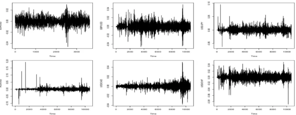
Figure 1: Time series plots for raw exchange rate data
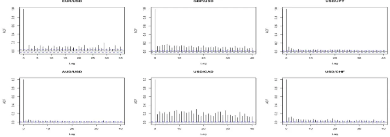
Figure 3: ACF for squared return series
that the return series are right-skewed and the distribution of the series may have fat tails. The time series plots of raw and return series datasets are also shown in Figures 1 and 2, respectively. Figure 3 shows the autocorrelation function (ACF) for the squared return series in each dataset. Except for AUD/USD, it is clear that the the squared series seem to be serially correlated.
Recall that yt=σtεtand εt has mean 0 and variance 1. Therefore, E(yt2) =E[E(yt2|Ft−1)] =E[E(σ2tε2t|Ft−1)] =σt2,
whereFt denotes the past financial information up to timet. Using this fact and since the true squared volatilityσ2t is unknown when we deal with the actual datasets, we use the squared series y2t as a proxy for the squared volatility. Hence, we measure MADE by MADE= 1 n n X t=1 |σˆ2t −yt2|= 1 n n X t=1 at
where at =|σˆ2t −y2t|. As another measure of accuracy, we use the directional accuracy (DA) defined by DA= 1 n n X t=1 dt, (15) where dt= ( 1, if (y2t −y2t−1)(ˆσt2−σˆt2−1)>0, 0, otherwise.
The DA gives the average direction of the forecast volatility by measuring the correctness of the turning point forecasts.
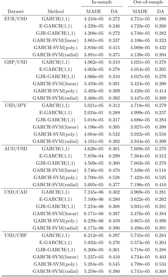
We report the results in Table 3. It is clear that GARCH-SVM outperforms the existing GARCH models. To test for forecasting accuracy, we carried out the one-sided Diebold and Mariano (DM) test proposed by Diebold and Mariano (1995). The underlying hypotheses associated with this test are
Table 3: In-sample and out-of-sample measures are shown.
In-sample Out-of-sample
Dataset Method MADE DA MADE DA
EUR/USD GARCH(1,1) 4.210e-05 0.272 4.751e-05 0.286 E-GARCH(1,1) 4.220e-05 0.246 4.723e-05 0.260 GJR-GARCH(1,1) 4.208e-05 0.272 4.748e-05 0.282 GARCH-SVM(linear) 3.861e-05 0.337 4.106e-05 0.323 GARCH-SVM(poly.) 3.856e-05 0.415 4.089e-05 0.432 GARCH-SVM(radial) 3.891e-05 0.375 4.139e-05 0.394 GBP/USD GARCH(1,1) 4.062e-05 0.310 4.021e-05 0.278 E-GARCH(1,1) 4.003e-05 0.278 4.054e-05 0.265 GJR-GARCH(1,1) 4.066e-05 0.310 4.027e-05 0.276 GARCH-SVM(linear) 3.459e-05 0.391 3.424e-05 0.390 GARCH-SVM(poly.) 3.493e-05 0.399 3.420e-05 0.414 GARCH-SVM(radial) 3.468e-05 0.392 3.447e-05 0.389 USD/JPY GARCH(1,1) 5.021e-05 0.312 4.718e-05 0.279 E-GARCH(1,1) 2.024e-01 0.289 4.999e-05 0.257 GJR-GARCH(1,1) 5.018e-05 0.317 4.686e-05 0.283 GARCH-SVM(linear) 4.196e-05 0.395 3.927e-05 0.398 GARCH-SVM(poly.) 4.084e-05 0.532 3.922e-05 0.558 GARCH-SVM(radial) 4.191e-05 0.392 3.944e-05 0.399 AUD/USD GARCH(1,1) 4.626e-05 0.301 7.609e-05 0.270 E-GARCH(1,1) 7.859e-04 0.299 7.384e-05 0.312 GJR-GARCH(1,1) 4.509e-05 0.300 7.603e-05 0.270 GARCH-SVM(linear) 3.746e-05 0.470 7.349e-05 0.518 GARCH-SVM(poly.) 3.700e-05 0.528 7.422e-05 0.525 GARCH-SVM(radial) 3.695e-05 0.377 7.196e-05 0.410 USD/CAD GARCH(1,1) 7.245e-06 0.302 3.969e-05 0.281 E-GARCH(1,1) 7.100e-06 0.280 3.622e-05 0.262 GJR-GARCH(1,1) 7.224e-06 0.308 3.931e-05 0.281 GARCH-SVM(linear) 6.171e-06 0.397 3.476e-05 0.384 GARCH-SVM(poly.) 6.229e-06 0.459 3.867e-05 0.398 GARCH-SVM(radial) 6.175e-06 0.390 3.498e-05 0.391 USD/CHF GARCH(1,1) 6.212e-05 0.297 5.745e-05 0.284 E-GARCH(1,1) 5.932e-05 0.276 5.573e-05 0.264 GJR-GARCH(1,1) 6.200e-05 0.301 5.718e-05 0.288 GARCH-SVM(linear) 5.237e-05 0.410 4.734e-05 0.403 GARCH-SVM(poly.) 5.284e-05 0.545 4.798e-05 0.534 GARCH-SVM(radial) 5.258e-05 0.380 4.741e-05 0.368
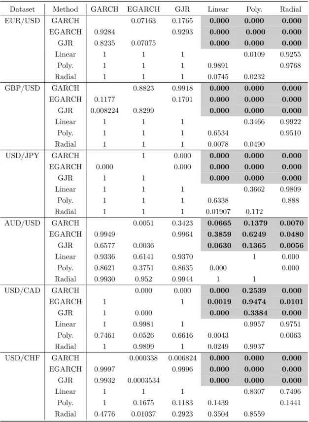
Table 4: Diebold-Mariano (DM) test. The entries are the p-values from the test.
Dataset Method GARCH EGARCH GJR Linear Poly. Radial
EUR/USD GARCH 0.07163 0.1765 0.000 0.000 0.000 EGARCH 0.9284 0.9293 0.000 0.000 0.000 GJR 0.8235 0.07075 0.000 0.000 0.000 Linear 1 1 1 0.0109 0.9255 Poly. 1 1 1 0.9891 0.9768 Radial 1 1 1 0.0745 0.0232 GBP/USD GARCH 0.8823 0.9918 0.000 0.000 0.000 EGARCH 0.1177 0.1701 0.000 0.000 0.000 GJR 0.008224 0.8299 0.000 0.000 0.000 Linear 1 1 1 0.3466 0.9922 Poly. 1 1 1 0.6534 0.9510 Radial 1 1 1 0.0078 0.0490 USD/JPY GARCH 1 0.000 0.000 0.000 0.000 EGARCH 0.000 0.000 0.000 0.000 0.000 GJR 1 1 0.000 0.000 0.000 Linear 1 1 1 0.3662 0.9809 Poly. 1 1 1 0.6338 0.888 Radial 1 1 1 0.01907 0.112 AUD/USD GARCH 0.0051 0.3423 0.0665 0.1379 0.0070 EGARCH 0.9949 0.9964 0.3859 0.6249 0.0480 GJR 0.6577 0.0036 0.0630 0.1365 0.0056 Linear 0.9336 0.6141 0.9370 1 0.000 Poly. 0.8621 0.3751 0.8635 0.000 0.000 Radial 0.9930 0.952 0.9944 1 1 USD/CAD GARCH 0.000 0.000 0.000 0.2539 0.000 EGARCH 1 1 0.0019 0.9474 0.0101 GJR 1 0.000 0.000 0.3384 0.000 Linear 1 0.9981 1 0.9957 0.9751 Poly. 0.7461 0.0526 0.6616 0.0043 0.0063 Radial 1 0.9899 1 0.0249 0.9937 USD/CHF GARCH 0.000338 0.006824 0.000 0.000 0.000 EGARCH 0.9997 0.9996 0.000 0.000 0.000 GJR 0.9932 0.0003534 0.000 0.000 0.000 Linear 1 1 1 0.8307 0.7496 Poly. 1 0.1675 0.1183 0.1439 0.1441 Radial 0.4776 0.01037 0.2923 0.3504 0.8559
H0 :E(at)row =E(at)column vs. H1 :E(at)row > E(at)column, whereat=|ˆσt2−y2t|.
Table 4 gives the results from this DM test. Each p-value in the table indicates the significance of the model in the row versus the model in the column. For each dataset in the table, we are particularly interested in the upper triangle of the matrix, especially, the bold and highlighted p-values. We can see that GARCH-SVM forecasts are better than GARCH, E-GARCH, and GJR-GARCH except for AUD/USD and USD/CAD datasets. This may result from the fact that these two datasets have high kurtosis. However, the radial basis kernel function seems to accommodate this and the GARCH-SVM significantly outperforms in all datasets.
5 Conclusion
In this paper, we attempted to estimate the volatility using the support vector ma-chine based on GARCH(1,1)-framework. Overall, this attempt was successful in both simulations and real data examples. Empirical studies have shown that heavy-tailed distribution is evident in many financial time series datasets. To account for this, we used the t-distribution with 3 degrees of freedom. We noted that GARCH-SVM works pretty well under the heavy-tailed distribution as wells as the normal distribution.
We used six different foreign exchange rate datasets to examine the GARCH-SVM model and we noted that polynomial-based GARCH-SVM significantly gives better pre-dictive potential in four out of six datasets; the linear-based model gives better potential in five out of six datasets; the radial basis gives better potential in all six datasets. While there is no literature on selecting an optimal kernel function, we found that if the dataset has a very high kurtosis the radial basis function works the best.
References
Bollerslev, T. (1986). Generalized autoregressive conditional heteroskedasticity. Journal of Econometrics, 31, 307-327.
Bollerslev, T. (2008). Glossary to ARCH (GARCH). CREATES Research Paper 49. Bollerslev, T., and Wooldridge, J. M. (1992) Quasi-maximum likelihood estimation and
inference in dynamic models with time-varying covariances. Econometric Reviews, 11, 143-172.
Chen, S., Hardle, W. K., and Jeong, K. (2010) Forecasting Volatility with Support Vector Machine-Based GARCH Model. Journal of Forecasting, 29, 406-433.
Diebold F., and Mariano R. (1995) Comparing predictive accuracy. Journal of Business and Economic Statistics, 13, 253-265.
Engle, R. (1982). Autoregressive conditional heteroskedasticity with estimates of the variance of United Kingdom inflations. Econometrica, 50, 987-1007.
Fletcher, R. (1987). Practical Methods of Optimization. New York: Wiley.
Glosten, L. R., Jagannathan, R., and Runkle, D. E. (1993). On the relation between the expected value and the volatility of nominal excess return on stocks. Journal of Finance,48, 1779-1801.
Gokcan, S. (2000). Forecasting volatility of emerging stock markets: linear versus non-linear GARCH models. Journal of Forecasting, 19(6):499?504.
Hansen, P. R. and Lunde, A. (2005). A forecast comparison of volatility models: Does anything beat a GARCH(1,1)? Journal of Applied Econometrics, 20:873?889.
Malmsten, H., and Ter¨asvirta, T. (2004). Stylized facts of financial time series and three popular models of volatility. SSE/EFI Working Paper Series in Economics and Finance, 563.
Nelson, D. B. (1991). Conditional heteroskedasticity in asset returns: A new approach.
Econometrika, 59, 347-370.
Ou, P., and Wang, H. (2010). Financial Volatility Forecasting by Least Square Sup-port Vector Machine Based on GARCH, EGARCH, and GJR Models: Evidence from ASEAN Stock Markets. International Journal of Economics and Finance, 2(1), 51-64. Perez-Cruz, F., Afonso-Rodriguez, J. A., and Giner, J. (2003). Estimating GARCH
models using support vector machines. Quantitative Finance, 3, 1-10.
Rydberg, T. H. (2000). Realistic Statistical Modelling of Financial Data. International Statistical Review, 68(3), 233-258.
Sch¨olkopf, B., and Smola, A. (2001). Learning with Kernels. MIT Press, Cambridge, MA.