HAL Id: hal-02288293
https://hal.archives-ouvertes.fr/hal-02288293
Submitted on 14 Sep 2019
HAL
is a multi-disciplinary open access
archive for the deposit and dissemination of
sci-entific research documents, whether they are
pub-lished or not. The documents may come from
teaching and research institutions in France or
abroad, or from public or private research centers.
L’archive ouverte pluridisciplinaire
HAL
, est
destinée au dépôt et à la diffusion de documents
scientifiques de niveau recherche, publiés ou non,
émanant des établissements d’enseignement et de
recherche français ou étrangers, des laboratoires
publics ou privés.
Randomshot, a fast nonnegative Tucker factorization
approach
Abraham Traoré, Maxime Berar, Alain Rakotomamonjy
To cite this version:
Abraham Traoré, Maxime Berar, Alain Rakotomamonjy. Randomshot, a fast nonnegative Tucker
factorization approach. 2019. �hal-02288293�
factorization approach
Abraham Traor´e, Maxime Berar, and Alain Rakotomamonjy
University of Rouen-Normandie,76000 Rouen, France [email protected]
{maxime.berar,alain.rakotomamonjy}@univ-rouen.fr
Abstract. Nonnegative Tuckerdecomposition is a powerful tool for the extraction of nonnegative and meaningful latent components from a positive multidimensional data (or tensor) while preserving the natural multilinear structure. However, as a tensor data has multiple modes, the existing approaches suffer from a high complexity in terms of compu-tation time since they involve intermediate compucompu-tations that can be time consuming. Besides, most of the existing approaches for nonnega-tiveTuckerdecomposition, inspired from well-established Nonnegative Matrix Factorization techniques, do not actually address the convergence issue. Most methods with a convergence rate guarantee assume restrictive conditions for their theoretical analyses (e.g. strong convexity, update of all of the block variables at least once within a fixed number of iterations). Thus, there still exists a theoretical vacuum for the convergence rate problem under very mild conditions.
To address these practical (computation time) and theoretical (conver-gence rate under mild conditions) challenges , we propose a new iterative approach namedRandomshot, which principle is to update one latent factor per iteration with a theoretical guarantee: we prove, under mild conditions, the convergence of our approach to the set of minimizers with high probability at the rateO 1
k
,kbeing the iteration number. The effectiveness of the approach in terms of both running time and solution quality is proven via experiments on real and synthetic data.
Keywords: nonnegativeTucker·convergence rate·proximal gradient
1
Introduction
The recovery of information-rich and task-relevant variables hidden behind data (commonly referred to as latent variables) is a fundamental task that has been extensively studied in machine learning [19],[6],[10]. In many applications, the dataset we are dealing with naturally presents different modes (or dimensions) and thus, can be naturally represented by multidimensional arrays (also called tensors). The recent interest for efficient techniques to deal with such datasets is motivated by the fact that the methodologies that matricize the data and then apply well-known matrix factorization techniques give a flattened view of the data and often cause a loss of the internal structure information [6], [19]. Hence,
to mitigate the extent of this loss, it is more favourable to process a multimodal data set in its own domain, i.e. tensor domain, to obtain a multiple perspective view of the data rather than a flattened one [19].
Tensor decomposition techniques are promising tools for exploratory analysis of multidimensional data in diverse disciplines including signal processing [2], social networks analysis [8]. In this paper, we focus on a specific tensor factorization, that is, the Tucker decomposition with nonnegativity
constraints. The Tucker decomposition, established by Tucker [16], is one
of the most common decompositions used for tensor analysis with many real applications [17], [12].
Most of the approaches for the nonnegative Tucker problem are derived from some existing standard techniques for theNonnegative Matrix Factorization NMF (i.e. they are natural extensions of these techniques) and do not provide any convergence guarantee (i.e. theoretical convergence proof). An iterative approach, inspired from the so-calledHierarchical Least Squares has been proposed in [12] . The idea is about employing ”local learning rules”, in the sense that the rows of the loading matrices are updated sequentially one by one. The main limitation of this method is the lack of convergence guarantee and the update of all of the variables, which can be time consuming. The class ofNMF-based methods emcompasses other approaches such as those set up in [10], [6], etc.
Alongside the NMF-based approaches, some Block Coordinate Descent-type algorithms have been proposed. Roughly speaking, the idea is to cyclically update the variables (i.e. update of all of the block variablesper iteration or in every fixed number of iterations in a deterministic or random order). A method proposed in [17] ensures a convergence rate (to a critical point) and imposes for the convergence analysis, the strong convexity assumption of each block-wise function (i.e. a multivariate function considered as a function of only one variable) for some of the update schemes proposed. This method can be time-consuming due to the update of all of the block variables per iteration. Besides, the block-wise strong convexity is not always verified [3]. A second approach estab-lished in [18], ensures a convergence rate (to a critical point) with no convexity assumption, but for the convergence analysis, it requires for all of the block
variablesto be updated (in a cyclic order or with a random shuffling) in every
fixed number of iterations. Thus, there is still a theoretical vacuum for approaches yielding convergence rates under loose conditions (i.e. without any convexity-type assumption [17], any constraint for all of the variables to be updated per iteration [17] or at least once within a fixed number of iterations [18], any full-rankness [3] assumption).
The method set up in this paper, based on the update per iteration of a single block variable picked randomly, can be classified among theRandomized Proximal Coordinate Gradient-type methods [9]: we propose an algorithm for which each update is performed via a single iteration ofProjected Gradient Descent with the
descent step defined via a carefully chosen minimization problem . Our approach is different from the Block Coordinate Descent, which idea is to update all of the variables (per iteration [17], [3] or in every fixed number of iterations [18]). With regards to the existing works for nonnegativeTuckerdecomposition, our contributions are the following ones:
– Proposition of a fast randomized algorithm for the nonnegativeTucker prob-lem, namedRandomshotfor which each update stage can be parallelized, – Theoretical guarantee: we prove with high probability, under fairly loose conditions (i.e. with no convexity assumption, no constraint for all of the variables to be updated and no rank-fullness assumption), the convergence to the set of minimizers at the rateO 1
k
,kbeing the iteration number. – Numerical experiments are performed to prove the efficiency of our approach
in terms of running time and solution quality.
2
Notations
A N−order tensor is denoted by a boldface Euler script letterX ∈RI1×···×IN.
The entries ofX ∈RI1×..×IN are denoted byX
i1,..,iN. The matrices are denoted
by bold capital letters (e.g.A). The identity matrix is denoted byId. The jth
row of a matrixA∈RJ×L is denoted byA
j,: and the transpose of a matrixA
byA>. The Hadamard product (or component-wise product) of two matrices of the same dimensions A andB is denoted by AB. Matricization is the process of reordering all the elements of a tensor into a matrix. The mode-n
matricization of a tensor [X](n) arranges the mode-n fibers to be the columns of the resulting matrixX(n)∈
RIn×( Q
m6=nIm). The mode-nproduct of a tensor
G ∈RJ1×···×JN with a matrix A∈
RIn×Jn denoted by G×nA yields a tensor
of the same order B∈RJ1×···Jn−1×In×Jn+1···×JN whose mode-nmatricized form
is defined by: B(n) = AG(n). For a tensor X ∈
RI1×...×IN, its ith
n subtensor
with respect to the modenis denoted byXnin∈RI1×···×In−1×1×In+1×···×IN and
defined via the mapping between its n-mode matricization
Xnin
(n)
and theith n
row of X(n), i.e. the tensorXn
in is obtained by reshaping the i
th
n row ofX(n),
with the target shape (I1, .., In−1,1, In+1, .., IN) (e.g. the second subtensor with
respect to the third mode of X ∈R20×30×40 is the tensor X32 ∈ R20×30 with X3
2
i,j=Xi,j,2,1≤i≤20,1≤j≤30). TheN−orderidentity tensor of size
R is denoted byI ∈RR×...×R and is defined by:Ii1,i2,..,iN = 1 ifi1 =..=iN
and 0 otherwise.
For writing simplicity, we introduce the following notations:
– The set of integers from n to N (with n and N included) is denoted by In
N ={n, ., N}. Ifn= 1, it is simply denoted byIN ={1, .., N}.
– We denote byIpN6=n={p, .., n−1, n+ 1, .., N}the set of integers frompto
N withnexcluded. Ifp= 1, this set will be simply denoted byIN6=n.
The product ofG with the matricesA(m)will also be alternatively expressed by: G ×m m∈IN A(m) = G × m m∈In−1 A(m)× nA(n) ×q q∈InN+1 A(q) =G × m m∈IN6=n A(m)× nA(n)
The Frobenius norm of a tensorX ∈RI1×···×IN, denoted bykXk F is defined by: kXkF = P 1≤in≤In,1≤n≤NX 2 i1,···,iN 12
. The same definition holds for matrices. The`1norm for tensor, denoted byk · · · k1is defined by:kXk1=Pi1,..,iN|Xi1,..,iN|.
The maximum and minimum functions are respectively denoted by max and min. We denote the positive part of a tensor by (X)+, i.e. (X)+= max(X,0) with max(.,0) applied component-wise. The same definition holds for matrices. The proximal operator of a functionf, denotedProxf is defined by:
Proxf(x) = arg minu f(u) +
1
2ku−xk 2
F
The indicator function and the complement of a setAare denoted by1AandAc.
The notationRI+ represent the elements ofRI with positive components.
3
Fast nonnegative Tucker
3.1 Nonnegative Tucker problem
Given a positive tensor X ∈ RI1×...×IN (i.e. with nonnegative entries), the
nonnegativeTuckerdecomposition aims at the following approximation:
X ≈G ×m m∈IN
A(m),G∈RJ+1×...×JN,A (m)∈
RI+m×Jm
The tensorGis generally called the core tensor and the matricesA(m)the loading
matrices: we keep these denotations for the remainder of the paper. A natural way to tackle this problem is to inferG andA(m) in such a way that the discrepancy
betweenX andG ×m m∈IN
A(m) is low. Thus, a relevant problem is:
min G≥0,A(1)≥0,···,A(N)≥0 fG,A(1),· · ·,A(N)=4 1 2kX−Gm∈×mIN A(m)k2 F (1)
3.2 Randomshot, a randomized nonnegative Tucker approach
Contrary to the existing approaches for nonnegative Tucker problem, based either onNMF extension [12] orBlock Coordinate Descent (update of all of the variables per iteration [17] or within a fixed number of iterations [18]), the idea of our approach namedRandomshot, is based on the update of only one variable per iteration picked randomly while fixing the others at their last updated values. Each update is performed via a single iteration of Projected Gradient Descent. To avoid an unnecessary distinction between the core tensorG and the loading matricesA(m), we rename the variablesG,A(1), ...A(N)byx
1, x2, ..., xN+1:
x1=G, xj+1=A(j),1≤j≤N (2)
Besides, we denote byxk
j the value of the variablexj at thekthiteration. With
these notations and by denoting the derivative of the functionf with respect to
xi by∂xif, the principle of Randomshotis summarised byAlgorithm 1.
Remark 1. The equality in Algorithm 1is due to the fact thatProx1A with
Algorithm 1Randomshot
Inputs:X: tensor of interest,n: splitting mode,x01≡G0: initial core tensor, n x0 m+1≡A (m) 0 o 1≤m≤N
: initial loading matrices.
Output:G∈RJ+1×...×JN,A
(m)∈
RI+m×Jm,1≤m≤N Initialization:k= 0
1: whilea predefined stopping criterion is not metdo
2: Choose randomly indexi∈ {1, ..., N+ 1}a with a probabilitypi>0
3: Compute optimal stepηi
k via the problem defined by the equation (7).
4: Block variable update
xki+1= xki −η i k∂xif(x k 1, ..., x k N+1) + =Prox1 RI+ xki −η i k∂xif(x k 1, ..., x k N+1)
withIbeing the dimension ofxi,1RI
+ the indicator function ofR
I + 5: xk+1 j =x k j,∀j6=i 6: k←k+ 1 7: end while
3.3 Efficient computation of the gradient via parallelization
For the computation of the block-wise derivatives, we propose a divide-and-conquer approach: we split the data tensor into independent sub-parts and determine the gradients via the computation of independent terms involving these sub-parts. For a fixed integer 1≤n≤N (in the sequel,nwill be referred to as the splitting mode), this is achieved via the following reformulation of the objective function in terms of subtensors drawn with respect to thenth mode
(seeProperty 1in the supplementary material):
f(G,A(1), ..,A(N)) = In X in=1 1 2kX n in−G ×m m∈IN6=n A(m)×nA (n) in,:k 2 F (3)
The tensorXnin is thei
th
n subtensor with respect to the splitting moden.
From the equation (3), each derivative inAlgorithm 1 can be computed via a parallelization process. To observe this, we distinguish three cases: deriva-tive with respect to the core tensor G, derivative with respect toA(p), p 6=n,
derivative with respect toA(n) withnbeing the splitting mode.
First case: derivative with respect to the core. The derivative with respect to the core is given by (see Property 5 in the supplementary material):
∂Gf Gk,A (1) k , ..,A (N) k = In X in=1 Rin ×m m∈IN6=n A(km) > ×n A(kn) in,: > | {z } θin (4) withRin=−X n in+Gk ×m m∈IN6=n A(km)×n A(kn) in,:
ofIn independent terms, it can be computed via a parallelization process.
Second case: derivative with respect to A(p), p6=n. The derivative with
respect to A(p) is given by (seeProperty 7 in the supplementary material):
∂A(p)f Gk,A (1) k , ..,A (N) k = In X in=1 − Xnin (p) +A(kp)B(inp) B(inp) > (5) The matrices (Xn in) (p) andB(p)
in represent respectively the mode-pmatricized
forms of theith
n subtensorX n
in and the tensorBin is defined by :
Bin =Gk ×m m∈Ip−1 A(km)×pId ×q q∈IpN+16=n A(kq)×n A(kn) in,: ,Id∈RJp×Jp: identity
This derivative being the sum ofIn independent terms, its computation can also
be parallelized.
Third case: derivative with respect to A(n). The derivative with respect to
A(n)can be computed via the row-wise stacking ofIn independent terms, that
are the derivatives with respect to the rowsA(j,n:), which allows to determine it via a parallelization process. Given the expression off given by (3),∂A(n)
j,:
f depends on a single subtensorXn
j and is given by (seeProperty 6 in the supplementary):
∂A(n) j,: fGk,A (1) k , .,A (N) k =− (Xnj)(n)−A(kn) j,: B(n) B(n)> (6) The matrices (Xn j)(n)∈R 1×Q
k6=nIk andB(n) respectively represent the mode-n
matricized form of the tensorsXn
j andB=Gk ×m m∈IN6=n
A(km).
4
Framework of the theoretical analysis
For the analysis, we consider a framework where a single variable is updated per iteration. The justification of this theoretical analysis with re-spect to existing analyses performed for theRandomized Proximal Coordinate Gradient approaches stems from the fact that either they assume the convexity of the objective function [1] or present different algorithmic settings [9], which make their analyses non applicable to our setting. We recall that our objective in this paper is not to compete withRandomized Proximal Coordinate Gradient
methods, but to fill the theoretical vaccum for the nonnegativeTuckerproblem. For simplicity purpose, we consider the alternative notations given by the equa-tion (2) as well as the following notaequa-tions:
A. The objective function evaluated at xk1, .., xkN+1 (i.e. the value of the
vari-ables at the iterationk) is denoted byf(xk). The same notation holds for any
function of the variables
xk
1, .., xkN+1 , with xkj being the value of xj at the
B. The objective function evaluated at xk 1, .., xki−1, x k+1 i , x k i+1, .., xkN+1 will be denoted byf(xk 1, .., xki−1, x k+1 i , xki+1, .., xkN+1). C.Γi = maxD1×D2×...DN+1k∂xif(x1, .., xN+1)kF: supremum ofk∂xifkF on D1×
...DN+1 with ×referring to the Cartesian product and the set Dj defined in
the subsection 4.2.Γi is well defined sincek∂xifkF is continuous and the finite
product of compact sets is a compact set. D.Γ = max(Γi,1≤i≤N+ 1)
Our theoretical analysis is mainly based on a careful definition of the descent steps (see section 4.1) as well as some natural assumptions (see section 4.2).
4.1 Definition of the descent step ηi
k at the (k+ 1)
th iteration
By assuming that at the iterationk+ 1, theithvariable has been selected, we
introduce the following definition ofηk i: ηik= arg min η∈[√δ1 K, δ2 √ K] η−√δ1 K max (Φ(η), Ψ(η), θ(η)) (7) Φ(η) =f(xk1, .., xi−k 1, xki −η∂xif(x k) +, x k i+1, .., x k N+1)−f(x k) 1−f(x k) 2 (8) Ψ(η) =k xki −η∂xif x k +−x k ik 2 F−η 2k∂ xif(x k)k2 F (9) θ(η) =h∂xif(x k ),(xki −η∂xif(x k ))+−xkii (10) +λfxk1, .., xki−1, xki −η∂xif(x k) +, x k i+1, .., x k N+1
The parameters λ > 0, δ2 > δ1 > 0 represent user-defined parameters, K
represents the maximum number of iterations. The problem (7) is well defined since it corresponds to the minimization of a continuous function on a compact set, byAssumption 4(presented in the section 4.2) and by the fact that all of the factors
xk
1, .., xkN+1 are already known at the (k+ 1)thiteration. Besides,
it corresponds to the minimization of a unimodal function for which there are several resolution heuristics such as theGolden section method.
4.2 Assumptions
Besides of the definition (7), we consider the following five assumptions:
Assumption 1. thenth subtensors are uniformly bounded: kXn
jkF ≤σ,∀j.
Assumption 2. we consider the domainG∈D1,A(m)∈Dm+1 with:
D1= Ga ∈RJ1×...×JN|kGakF ≤α ,Dm+1= n A(am)∈RIm×Jm|kA(am)kF ≤α o
Assumption 3. the solution of the problem (7) is not attained at √δ1 K: δ1 √ K < η i k≤ δ2 √ K (11)
Assumption 4. non-vanishing gradient
∂xif(x
k)6= 0 (12)
Assumption 5. minimizer not attained at the initial point
f(x01, .., x0N+1) =f(x0)=6 fmin, fmin:minimum of f onD1×...×DN+1 (13)
4.3 Theoretical result
Under the definition of the minimization problem given by (7) and the assumptions laid out in the section 4.2, the following inequality holds:
∀k >2 maxk0,21 + log(1ρ)− 2 ∆0 + 2 with 0< ρ <1, 0< <min(2, ∆0): 1−ρ≤P ∆k ≤ 2 k−2k0 +α 2Nδ2 2Γ2 λk (14) with log being the logarithmic function,k0= log(1+1 λ)log
1 log(1+λ)
(λ >0 being the parameter that intervenes in the problem (7)), ∆k = f xk
−fmin ≥ 0,
fmin being the minimum value off onD1×D2×..×DN+1:fmin well defined
sincef is continuous and a finite product of compact sets is a compact set. The probabilityPis the sampling distribution of the block variables inAlgorithm 1. This result states that the random sequence xk =
xk
1, .., xkN+1 converges to
the set of minimizers of the function f (given by (1)) at the rateO(1k) with a probability at least 1−ρ.
To establish this result, we consider a sequence of properties that are Property 1, Property 2, Property 3, Property 4, Property 5. The proof of Property 4 and the Lipschitz character of the block-wise derivatives (used by Property 2) are postponed in the supplementary (since they are perfectly straightforward) as well as some inequalities for Property 1 (to avoid arguments redundancy).
Property 1. By considering that theithvariable has been picked at the(k+ 1)th
iteration, the following inequalities hold:
f(xk+1)≤f(xk) 1−f(x k) 2 (15) kxki+1−xkik2 F ≤(η i k) 2k∂ xif(x k)k2 F (16) h∂xif(x k), xk+1 i −x k ii ≤ −λf(x k+1) (17)
The inequality (15) ensures the decreasing of the objective function after each update. The intuition of the inequality (16) is that it yields an estimation of the Lipschitz parameter of the functionx→∂xif(x
k
1, ., xki−1, x, xki+1, ., xkN+1).
The inequality (17) controls the random character of the gradient by carefully choosing the descent directionxki+1−xk
Proof: by definition ofηi
k as a minimizer (equation (7)), we have:
(ηi k− δ1 √ K) max Φ η i k , Ψ ηi k , θ(ηi k) ≤(√δ1 K− δ1 √ K) max Φ√δ1 K , Ψ√δ1 K , θ(√δ1 K) By Assumption 3,ηi k > δ1 √
K. Thus, the previous inequality yields:
max Φ ηi k , Ψ ηi k , θ(ηi k) ≤0⇒Φ ηi k ≤0 andΨ ηi k ≤0 andθ(ηi k)≤0.
The inequalities (15), (16), (17) stem fromΦ ηik≤0,Ψ ηik≤0,θ(ηki)≤0. Since the reasoning is identical for the three inequalities, we perform it only for the first one (seeProperty 8 in the supplementary for the remaining ones). Given thatΦ ηi k ≤0, we have: f(xk 1, .., xki−1, xki −ηki∂xif(x k) +, x k i+1, .., xkN+1)−f(xk)(1− f(xk) 2 )≤0. Sincexki+1= xk i −ηik∂xif(x k) + by definition, we have: f(xk1, .., xki−1, x k+1 i , x k i+1, .., xkN+1)≤f(xk) 1−(f(x k) 2 (18) Asxkj+1=xkj forj 6=iby definition, the inequality (18) yields the result:
f(xk+1) =f(xk+1 1 , .., x k+1 i−1, x k+1 i , x k+1 i+1, .., x k+1 N+1)≤f(x k)(1−(f(xk)) 2 )
Property 2. The sequence∆k =f(xk)−fmin verifies the inequality:
∆k+1≤ ∆k
1 +λ+
α2Nδ22Γ2
2K(1 +λ) (19)
Proof: let’s consider xi the variable selected at the (k+ 1)th iteration. The
derivativex→∂xif(x
k
1, ., xki−1, x, xki+1, .., xkN+1) is Lipschitz (byProperty 4 and
Property 6 in the supplementary, each of them usingAssumptions 1 and 2) with respect to the variablexi with the parameter α2N. Thus, we have by [13]
f(xk1, .., xki−1, x k+1 i , x k i+1, .., x k N+1)≤f(x k 1, .., xki−1, x k i, x k i+1, .., x k N+1) +h∂xif(x k), xk+1 i −xkii+ α2N 2 kx k+1 i −xkik2F. Given thatxkj+1=xk
j,∀j6=i(selection ofxi), the last inequality yields:
f(xk+1)−fmin | {z } ∆k+1 ≤f(xk)−fmin | {z } ∆k + h∂xif(x k), xk+1 i −x k ii | {z }
can be bounded by Property 1
+ α 2N 2 kx k+1 i −x k ik 2 F | {z }
can be bounded by Property 1
.
ByProperty 1,Assumption 3, the definitions of Γi (as the supremum of∂xif)
andΓ (as max(Γ1, .., ΓN)) respectively, the last inequality yields:
∆k+1≤∆k−λf(xk+1) +α 2N 2 η i k 2 Γi2≤∆k−λf(xk+1) + α2Nδ2 2 2K Γ 2 ⇒∆k+1≤∆k−λf(xk+1) +λfmin+ α2Nδ2 2 2K Γ 2=∆ k−λ∆k+1+ α2Nδ2 2 2K Γ 2 ⇒(1 +λ)∆k+1≤∆k+ α2Nδ2 2 2K Γ
2: which concludes the proof.
Property 3. Let’s considerP the probability distribution with respect to which
the block variables are drawn andEP the expectation associated. Let’s consider the sequence∆k=f(xk)−fmin. Fork > 2
1 + log(1ρ)− 2
∆0 + 2(log being the
logarithmic function) with0< ρ <1,0< <min(2, ∆0). We have :
Proof: Claim 1: the sequence∆k is decreasing.
Justification of Claim 1: byProperty 1, we have:
∆k+1=f(xk+1)−fmin≤f(xk)−12 f(xk)
2
−fmin≤f(xk)−fmin=∆k
Claim 2:EP(∆k+1|∆k)≤∆k(1−∆2k),EP(|): the conditional expectation [14].
Justification of theClaim 2: byProperty 1we have:
f(xk+1)≤f(xk)−1 2 f(x
k)2
≤f(xk)−∆2k
2 (due to the fact 0≤∆k ≤f(x
k))
⇒∆k+1≤∆k− ∆2
k
2 (subtraction offmin on both sides of the last inequality)
⇒EP(∆k+1|∆k)≤∆k(1−∆2k) (property of the conditional expectation)
Given ∆0 > 0 (by Assumption 5), ∆k ≥ 0 (definition of fmin), Claim 1,
Claim 2 along with 0 < < ∆0 and < 2, we have (Theorem 1 in [14]):
P(∆k ≤)≥1−ρfork > 2
1 + log(1ρ)− 2
∆0 + 2
Property 4. Forpfixed and qsuch that p+q≤K, we can show that:
∆p+q≤ ∆p (1 +λ)q + α2Nδ2 2Γ2 2K q X j=1 1 (1 +λ)j ≤ ∆p (1 +λ)q + α2Nδ2 2Γ2 2Kλ (21)
Proof: this is perfectly straightforward and done by a simple reasoning by induction onq(forpfixed) usingProperty 2. (seeproperty 9 in the supplementary
material).
Property 5. For λ > 0 and k > k0 = log(1+1 λ)log
1 log(1+λ) , 1 (1+λ)k ≤ 1 k−k0
with logbeing the logarithmic function .
Proof: let’s consider the univariate function`(x) =x−exlog(1+λ)−k0defined on
the domainx > k0,ebeing the exponential function (inverse of the log function). The derivative is given by`0(x) = 1−(log(1 +λ))ex×ln(1+λ).
By definition ofeand given thatx > k0, log(1 +λ)>0 (sinceλ >0), we have:
xlog(1 +λ) ≥log 1 log(1+λ)
⇒ (log(1 +λ))exlog(1+λ) ≥1 ⇒ `0(x) ≤0: this
implies that`is a decreasing function on the domainx > k0. Thus, for an integerk > k0, we have:
`(k) =k−eklog(1+λ)−k0≤`(k0) =−ek0log(1+λ)<0
⇒0< k−k0< eklog(1+λ)= (1 +λ)k: this concludes the proof. Now, we establish the convergence to a minimizer with high probability.
Proof of our result given by the inequality (14)
We consider, k0, ρ, ∆k as for (14) andΛ= max
k0,21 + log(1ρ)− 2
∆0+ 2
. Without loss of generality, we consider thatΛ < K2 (we can chooseK sufficiently large such that this inequality is verified sinceΛis fixed in advance). Let’s choose
ksuch thatΛ < k≤ K
2 (suchkexists, e.g.k=
K 2). We have byProperty 4: ∆2k ≤ (1+∆λk)k + α2Nδ2 2Γ2 2λK ≤ ∆k k−k0 + α2Nδ2 2Γ2
2λk (since k ≤ K and Property 5:
applicable sincek > k0 due to the fact thatk > Λ≥k0) Given the implication∆k≤⇒∆2k≤ k−k
0 +
α2Nδ22Γ2
P(∆k≤)≤P ∆2k≤ k−k 0 + α2Nδ2 2Γ2 2λk Since k > 21 + log(1ρ)− 2
∆0 + 2 (due to the fact that k > Λ ), 0 < <
min(∆0,2),0< ρ <1, we have byProperty 3:
1−ρ≤P(∆k ≤)≤P(∆2k≤ k−k
0 +
α2Nδ2 2Γ2 2λk )
Let’s denoteh= 2k. Thus, ∀h >2 maxk0,2
1 + log(1ρ)− 2
∆0 + 2
,0< <
min(2, ∆0),0< ρ <1, the following inequality holds: 1−ρ≤P ∆h≤ 2 h−2k0 +α 2Nδ2 2Γ 2 λh
Remark 2. Contrary to the existing analyses for nonnegativeTucker, our proof
does not use any convexity assumption as in [17], does not impose for all of the block variables to be updated per iteration [17] or at least once within a fixed number of iterations as in [18] and does not assume any rank-fullness as in [3]. Besides, we prove the convergence to a minimizer for nonnegativeTuckerinstead of a critical point as it is the case for the state-of-the-art methods [17],[18], [3].
5
Numerical experiments
The objective of these experiments is to prove that our approach, based on the update of one variable picked randomly per iteration, yields competitive results both in terms of running time and solution quality compared to some state-of-the-artNMF-based andBlock Coordinate Descent-type (with all of the variables updated per iteration in a predefined order) approaches for the nonnegative
Tuckerproblem (which justifies the choice of the competitors presented
in the section 5.1). This demonstration is performed via some benchmark tasks: the objective is not to establish new techniques for these tasks, but to prove the efficiency of our approach in terms of computation time and solution quality.
5.1 Experimental setting
Randomshotis compared to the following five state-of-the-art methods:
1. TuckerLRA (Algorithm 1in [19]): this method is based on the
multiplica-tive update rules for the NMF and the replacement of the original tensor by a noise-reduced version.
2. TuckerHALS[19]: this approach is an extension of theHierarchical Least
Squares forNMF.
3. TuckerSparse[6]: this is an approach inspired from the multiplicative update
rules set up for theNMF problem.
4. TuckerCCD[17]: this approach proposes aBlock Coordinate Descent method
for the nonnegativeTuckerproblem with a convergence rate (to a critical point). Each block variable update is performed via an extrapolation operation.
5. CPCCD [17]: this is a standard method for the tensor completion problem
For all of the methods, the code has been done with Tensorly [7] except for
TuckerCCDandCPCCDfor which we recover the matlab code made
avail-able on the author’s [17] website for fairness purpose. For Randomshot, the derivatives computation is performed via the multiprocessing package ofPython
and the minimisation problems for the steps are solved by theGolden Section
method. As in [9], the variables are picked according to a uniform distribution on
{1, .., N+ 1},N: tensor order and only one variable is updated per iteration. For each experiment, the splitting modenis fixed to 1, i.e. we consider subtensors with respect to the first mode (changingnhas no effect onRandomshotoutput: it simply changes the way to compute the gradients, but not their final values).
5.2 Synthetic experiment
The task considered is the denoising problem of a three-order noisy tensor
Xn ∈ R300×200×100 defined by: Xn =Xreal+ 2×Noise withNoise = (N)+
andXreal= (T)+. The entries ofT andN are drawn from a standard Gaussian
distribution. For fairness purpose, the initial points and the stopping criterion are defined identically: each algorithm is stopped when the relative error is inferior to a predefined threshold or a maximum number of iterations is reached. The evaluation criteria are the running time and the reconstruction errorRe
defined by: Re=kXreal−Gout×1A (1) out×2A (2) out×3A (3)
outk2F withGout,
n
A(outn),1≤n≤3o being the latent factors inferred from the decomposition ofXn.
ForR∈ {5,7,10},{δ1, δ2}=10−6,10−5 and for the remaining values ofR,δ1
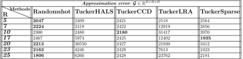
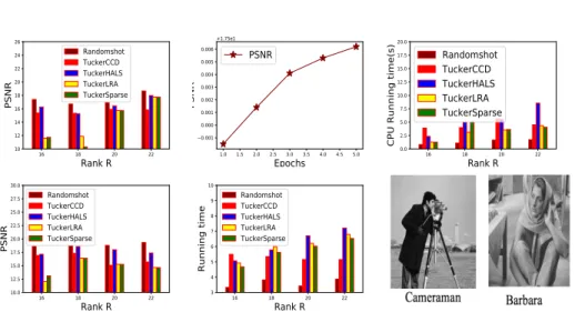
andδ2 are fixed to 10−7 and 10−6. The value ofλis fixed to 10−1for allR. Figure 1 portrays two expected behaviors of randomized-coordinate type algo-rithms, i.e. the decreasing of the objective function and the decreasing of the reconstruction error with respect to the number of epochs (one epoch=m con-secutive iterations withmbeing the number of block variables [4]). From Table 1 and Figure 1, our approach outperforms its competitors with less running time (other numerical results are provided in the section 6.2 of the supplementary).
5 7 10 17 20 23 25 Rank R 0 25 50 75 100 125 150 175 200
CPU Running Time (in seconds)
Randomshot TuckerLRA TuckerHALS TuckerCCD TuckerSparse 10 20 30 40 50 60 Epochs 7200 7400 7600 7800 8000 8200 8400 Reconstruction error
Reconstruction error per epoch
0 2 4 6 8 10 Running time 0.2 0.4 0.6 0.8 1.0 Objective function 1e8
Objective function vs running time
Fig. 1. Left: Running time (mean over 5 runs), Center: Reconstruction error with respect to the number of epochs, Right: Objective function with respect to time
Approximation error:G∈RR×R×R
R
Methods Randomshot TuckerHALS TuckerCCD TuckerLRA TuckerSparse
5 2047 2409 2421 2118 2564 7 2224 2418 2422 12919 2856 10 2300 2480 2180 31417 3970 17 2467 5974 2425 12402 1935 20 2213 30550 2427 21930 3412 23 2163 4246 2428 7613 2423 25 1806 6266 2428 23762 2181
Table 1.Reconstruction error (averaged over 5 independent runs)
5.3 Application to the impainting problem
We compare our approach to its competitors for the inpainting task, which aims to infer missing pixels in an image (we consider two images of size 256×256 and 512×512: see Figure 2). For this application, we build a training tensor
Strain ∈RNp×8×8 by stacking along the first mode overlapping patchesP
t of
size 8×8 (the number of patches being Np ∈ {32,64} for the two images)
constructed from the input image (with missing pixels). The core tensor as well as the loading matrices Al ∈ R8×R,Aw ∈ R8×R, Ae ∈ RNp×R (R being
an integer whose value has to be defined) are learned from Strain through a
nonnegative decomposition. Each patch is then reconstructed by estimating the sparse coefficients through the projection of the non-missing pixels on Aland
Aw matrices, i.e.Prt =Gt×1Al×2Aw with the components ofGt(defined as in
[11]) representing the sparse coefficients. The evaluation criteria are the running time for the decomposition ofStrain (i.e. the inference of the four latent factors
G,Al,Aw,Ae) and the PSNR defined by:
P SN R= 10 log10kIm×n×2552
real−Ireck2F
withm, nrepresenting respectively the image sizes and Ireal,Irec the real and the reconstructed images. Each evaluation
criterion is averaged over 5 independent selections of the non-missing pixels Again, we notice as expected, that our algorithm learns better with the number of epochs (one epoch being defined as in [4]). Our approach achieves greater PSNR within less time (Figure2) due its parallel and randomized natures. This proves
thatRandomshot, based on the update of a single variable picked randomly per
iteration, can be competitive with respect toNMF-based andBlock Coordinate Descent-type approaches for nonnegative Tuckerproblem.
5.4 Application to tensor completion problem
In this section, we consider a completion problem viaTuckerwith the core fixed to the identity tensorI∈RR×R×R. The problem of interest is given by [17]:
min A(1)∈RI1×R≥0,..,A(N)∈RIN×R≥0 kPΩ(X −I ×m m∈IN A(m))k2 F (22) withA(n)∈
RIn×R, Ω⊂[I1]×...×[IN], [In] representing the set of consecutive
16 18 20 22 Rank R 10 12 14 16 18 20 22 24 26 PSNR Randomshot TuckerCCD TuckerHALS TuckerLRA TuckerSparse 1.0 1.5 2.0 2.5 3.0 3.5 4.0 4.5 5.0 Epochs 0.001 0.000 0.001 0.002 0.003 0.004 0.005 0.006 PSNR +1.75e1 PSNR 16 18 20 22 Rank R 0.0 2.5 5.0 7.5 10.0 12.5 15.0 17.5 20.0
CPU Running time(s)
Randomshot TuckerCCD TuckerHALS TuckerLRA TuckerSparse 16 18 20 22 Rank R 10.0 12.5 15.0 17.5 20.0 22.5 25.0 27.5 30.0 PSNR Randomshot TuckerCCD TuckerHALS TuckerLRA TuckerSparse 16 18 20 22 Rank R 3 4 5 6 7 8 9 10 Running time Randomshot TuckerCCD TuckerHALS TuckerLRA TuckerSparse
Fig. 2. Top: results for Cameraman (image of size 256×256), Bottom: results for Barbara (image of size 512×512). Top left: PSNR , Top center: PSNR with respect to the number of epochs, Top right: Running time. Bottom left: PSNR, Bottom center: Running time (average of 5 independent runs). ForCameramanandBarbara, the values ofNp(number of patches) are fixed to 32 and 64. See supplementary forδ1, δ2, λ
operator PΩ keeps the entries which indexes belong toΩ and sets to zero the
remaining ones. We consider an equivalent formulation of (22) given by [17]: min Y,A(1)≥0,..,A(N)≥0,PΩ(X)=Y kY−I ×m m∈IN A(m)k2 F (23)
To solve the problem (23), we propose an extension of Algorithm 1 named
CPRandomshotcomp. The idea is to replace in Algorithm 1the tensorX
by an intermediate variableYk in the definition of the partial gradient and the
stepsηi
k (see section 5in the supplementary material fore more details). The
variableYk is updated just after theline 5in Algorithm 1via the equality:
Yk+1=PΩ(Yk) +PΩc I ×m m∈IN A(km+1) (24)
withkbeing to the iteration number. The difference between
CPRandomshot-compandCPCCDis the update scheme: for the first one, only one variable
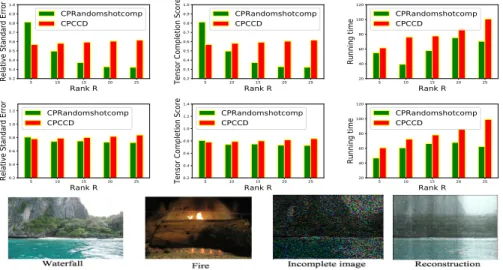
is updated per iteration. For the completion task, we consider two images, each being a tensorX ∈R500×500×3(see figure 3) provided by [5]. The tensor at hand
is split into a training and a test sets: 25% of entries are used for the inference of the latent factors and 75% are used for the test. For the evaluation criteria, we consider besides of the running time, two standard measures for a tensor completion problem that are theRelative Standard Error(RSE: the less the better) [15] and theTensor Completion Score (TCS: the less the better) [15]. Each evaluation criteria is averaged over 5 independent train−test splits.
5 10 15 20 25 Rank R 0.2 0.3 0.4 0.5 0.6 0.7 0.8 0.9 1.0
Relative Standard Error
CPRandomshotcomp CPCCD 5 10 15 20 25 Rank R 0.2 0.3 0.4 0.5 0.6 0.7 0.8 0.9 1.0
Tensor Completion Score
CPRandomshotcomp CPCCD 5 10 15 20 25 Rank R 20 40 60 80 100 120 Running time CPRandomshotcomp CPCCD 5 10 15 20 25 Rank R 0.2 0.4 0.6 0.8 1.0 1.2
Relative Standard Error
CPRandomshotcomp CPCCD 5 10 15 20 25 Rank R 0.2 0.4 0.6 0.8 1.0 1.2 1.4
Tensor Completion Score
CPRandomshotcomp CPCCD 5 10 15 20 25 Rank R 20 40 60 80 100 120 Running time CPRandomshotcomp CPCCD
Fig. 3.Top: results forWaterfall. Center: results forFire. From left to right: Relative Standard Error, Tensor completion Score and Running time with respect to the rank R. Bottom: images used and example of reconstruction forWaterfallby our approach
Our approach CPRandomshotcompperforms better than its competitor in terms of both solution quality and running time (see Figure 3). This proves nu-merically that the random selection of the variables along with the parallelization of the partial gradients can be competitive with respect to cyclic (deterministic)
Block Coordinate Descent in terms in solution quality within less running time (other numerical results are provided in the section 6.2 of the supplementary).
5.5 Additional experiments
In the section 7 of the supplementary, the robustness of our approach with respect to the step is proven, i.e. we demonstrate that if we fix the step instead of solving the problem (7), our approach still achieves competitive results. Besides, in the section 4 of the supplementary, we demonstrate that the non-vanishing gradient assumption (Assumption 4in the section 4.2) is verified in practice.
6
Conclusion
In this paper, we propose a new algorithm for the nonnegative Tuckerproblem for which we establish a convergence rate ofO 1
k
with high probability and prove that it achieves competitive results compared to some state-of-the-art nonnegative
Tuckerapproaches. Besides, we have proven numerically the robustness with
respect to the descent steps. Our future work entails the application of our approach principle to other types of decomposition different from Tucker as well the investigation of accelerated versions yielding better convergence rates for the nonnegativeTuckerproblem.
References
1. Alacaoglu, A., Tran-Dinh, Q., Fercoq, O., Cevher, V.: Smooth primal-dual coordi-nate descent algorithms for nonsmooth convex optimization. arXiv (2017) 2. Cichocki, A., Zdunek, R., Phan, A.H., Amari, S.i.: Nonnegative Matrix and Tensor
Factorizations: Applications to Exploratory Multi-way Data Analysis and Blind Source Separation. Wiley Publishing (2009)
3. Friedlander, M.P., Hatz, K.: Computing non-negative tensor factorizations. Opti-mization Methods Software23(4), 631–647 (2008)
4. G¨urb¨uzbalaban, M., Ozdaglar, A., Parrilo, P.A., Vanli, N.D.: When cyclic coordinate descent outperforms randomized coordinate descent. In: NIPS’17. pp. 7002–7010 (2017)
5. Jegou, H., Douze, M., Schmid, C.: Hamming embedding and weak geometric consistency for large scale image search. In: Proceedings of the 10th European Conference on Computer Vision: Part I. pp. 304–317 (2008)
6. Kim, Y.D., Choi, S.: Nonnegative tucker decomposition. 2007 IEEE Conference on Computer Vision and Pattern Recognition pp. 1–8 (2007)
7. Kossaifi, J., Panagakis, Y., Pantic, M.: Tensorly: Tensor learning in python. arXiv (2018)
8. Lin, C.Y., Cao, N., Xia Liu, S., Papadimitriou, S., Sun, J., Yan, X.: Smallblue: Social network analysis for expertise search and collective intelligence. ICDE pp. 1483 – 1486 (2009)
9. Lin, Q., Lu, Z., Xiao, L.: An accelerated randomized proximal coordinate gradient method and its application to regularized empirical risk minimization. SIAM Journal on Optimization25, 2244–2273 (2015)
10. Liu, J., Liu, J., Wonka, P., Ye, J.: Sparse non-negative tensor factorization using columnwise coordinate descent. Pattern Recogn.45(1), 649–656 (2012)
11. Lu, C., Shi, J., Jia, J.: Online robust dictionary learning. In: Proceedings of the 2013 IEEE Conference on Computer Vision and Pattern Recognition. pp. 415–422. CVPR ’13 (2013)
12. Phan, A.H., Cichocki, A.: Extended hals algorithm for nonnegative tucker decom-position and its applications for multiway analysis and classification. Neurocomput.
74(11), 1956–1969 (2011)
13. Reddi, S.J., Hefny, A., Sra, S., P´ocz´os, B., Smola, A.: Stochastic variance reduction for nonconvex optimization. pp. 314–323. ICML’16 (2016)
14. Richt´arik, P., Tak´aua´z, M.: Iteration complexity of randomized block-coordinate descent methods for minimizing a composite function. Math. Program.144(1-2), 1–38 (2014)
15. Song, Q., Ge, H., Caverlee, J., Hu, X.: Tensor completion algorithms in big data analytics. ACM Transactions on Knowledge Discovery from Data13(2017) 16. Tucker, L.R.: Implications of factor analysis of three-way matrices for
measure-ment of change. C.W. Harris (Ed.), Problems in Measuring Change, University of Wisconsin Press pp. 122–137 (1963)
17. Xu, Y., Yin, W.: A block coordinate descent method for regularized multiconvex optimization with applications to nonnegative tensor factorization and completion. SIAM J. Imaging Sciences6, 1758–1789 (2013)
18. Xu, Y., Yin, W.: A globally convergent algorithm for nonconvex optimization based on block coordinate update. J. Sci. Comput.72, 700–734 (2017)
19. Zhou, G., Cichocki, A., Zhao, Q., Xie, S.: Efficient nonnegative tucker decomposi-tions: Algorithms and uniqueness. IEEE Transactions on Image Processing24(12), 4990–5003 (2015)