Factor models of stock returns: GARCH errors versus time-varying betas

Phoebe Koundouri, Nikolaos Kourogenis, Nikitas Pittis,

Panagiotis Samartzis

Factor models of stock returns: GARCH

errors versus time-varying betas

Article (Accepted version)

(Refereed)

Original citation:

Koundouri, Phoebe, Kourogenis, Nikolaos, Pittis, Nikitas and Samartzis, Panagiotis (2016)

Factor models of stock returns: GARCH errors versus time-varying betas. Journal of Forecasting. ISSN 0277-6693

DOI: 10.1002/for.2387

© 2015 John Wiley & Sons, Ltd.

This version available at: http://eprints.lse.ac.uk/65548/

Available in LSE Research Online: February 2016

LSE has developed LSE Research Online so that users may access research output of the School. Copyright © and Moral Rights for the papers on this site are retained by the individual authors and/or other copyright owners. Users may download and/or print one copy of any article(s) in LSE Research Online to facilitate their private study or for non-commercial research. You may not engage in further distribution of the material or use it for any profit-making activities or any commercial gain. You may freely distribute the URL (http://eprints.lse.ac.uk) of the LSE Research Online website.

This document is the author’s final accepted version of the journal article. There may be differences between this version and the published version. You are advised to consult the publisher’s version if you wish to cite from it.

Factor Models of Stock Returns: GARCH Errors

versus Time - Varying Betas

Phoebe Koundouri

y

Nikolaos Kourogenis

z

Nikitas Pittis

z

Panagiotis Samartzis

z

Abstract

This paper investigates the implications of time-varying betas in factor models for stock returns. It is shown that a single-factor model (SFMT) with autoregressive betas and homoscedastic errors (SFMT-AR) is capable of reproducing the most important stylized facts of stock returns. An empirical study on the major US stock market sectors shows that SFMT-AR outperforms, in terms of in-sample and out-of-sample performance, SFMT with constant betas and conditionally heteroscedastic (GARCH) errors, as well as two multivariate GARCH-type models.

Keywords: autoregressive beta, stock returns, single factor model, conditional het-eroscedasticity, in-sample performance, out-of-sample performance.

JEL Classi…cation: C22, G10, G11, G12

Department of International and European Economic Studies, Athens University of Economics and Business and Grantham Research Institute on Climate Change and the Environment, London School of Economics and Political Science, UK.

y_{Correspondence to: Phoebe Koundouri, Department of International and European Economic} Studies, Athens University of Economics, 76, Patission Street, 104 34 Athens, Greece. Email: [email protected]. Tel: +302108203455.

1 Introduction

The analysis of the statistical properties of stock returns has been a research area of great interest since the beginning of 1950s. One of the most useful and intuitive statistical models for stock returns is the single factor model (SFM) which, together with its multivariate generalization (the multiple factor model), form the basis for many asset pricing models, such as the Arbitrage Pricing Model (APT), put for-ward by Ross (1976) or the Intertemporal Capital Asset Pricing Model (ICAPM), introduced by Merton (1973). The SFM attempts to capture the intuitive idea that asset returns are driven by unanticipated changes (surprises) of a common underly-ing factor. More speci…cally, in the context of SFM, the return, ri, of a security (or

a portfolio)i, i= 1;2; :::; n, is linearly related to an exogenous (zero-mean) variable

M through the linear regression ri = ai + iM +ui. The error term, ui, in this

model has zero mean, …nite variance and satis…es the condition E(ui jM) = 0, 8i = 1;2; :::; n. Furthermore, the theoretical assumption that the correlation be-tween ri and rj; i6=j stems solely from the common “causal” factor M entails the

assumption that Cov(ui; uj) = 0, for everyiandj; i6=j:The slope coe¢ cient, i, is

interpreted as a measure of the systematic risk of the stock i, and is usually referred to as the “beta coe¢ cient”, or simply the “beta” of the stock i.

SFM is a single period model. In the estimation of this model using time series data, it is usually assumed that the aforementioned linear relationship between ri;

i = 1;2; :::; n and M is time-invariant. Under this (often implicit) assumption, the stochastic process _fri;tg, i = 1;2; :::; n is probabilistically caused by the stochastic

process _fMtg through the temporal relationship ri;t = ai + iMt+ui;t, hereafter

referred to as SFMT, with _fui;tg being an iid process with zero mean and …nite

variance, 2

i. As a consequence, all the statistical properties offri;tg, i= 1;2; :::; n,

are determined solely by those of_fMtgand fui;tg. This means that SFMT is a

well-speci…ed statistical model and hence, empirically adequate. Empirical adequacy of SFMT means that the parameters ai, i and 2 are time-invariant, and the error

term ui;t is an iid process.

Has SFMT been found to be empirically adequate? The answer is negative. There are at least two sources for the empirical failure of SFMT. The …rst one lies in the fact that the error process_fui;tghas been found to exhibit temporal dependence,

which is usually identi…ed as conditional heteroscedasticity (CH). The second source of empirical inadequacy of SFMT comes from studies suggesting that the regression coe¢ cient i is not constant over time. Important studies o¤ering evidence for a

time-varying beta, i;t; include Blume (1971, 1975), Fabozzi and Francis (1978),

Fisher and Kamin (1985), Sunder (1980), Ohlson and Rosenberg (1982), Bos and Newbold (1984), Collins, Ledolter and Rayburn (1987), Bos and Fetherston (1992, 1995) and Fa¤, Lee and Fry (1992).

The response of the empirical literature to the aforementioned empirical fail-ures of SFMT has taken various forms among which the following two are the most prominent. The …rst response consists in replacing the assumption of independence of the error sequence with the assumption that _fui;tg exhibits non-linear

depen-dence, which usually takes the form of a GARCH-type model. Note that the re-sulting model, hereafter referred to as SFMT-GARCH, retains the (rather strong) assumption of a time-invariant beta. The second response focuses on the problem of beta instability, thus specifying models with stochastic parameters. For exam-ple, Shanken (1990) models the time varying beta as a linear function of observable state variables. Alternatively, the time varying beta is often treated as a stochastic (hidden) process. To this end, Fabozzi and Francis (1978) assumed that i;t is an

i.i.d process with …nite variance, while Fisher and Kamin (1985), Sunder (1980), Bos and Newbold (1984) and Jostova and Philipov (2005) allowed for persistence in the variation of beta by assuming that _i;t follows a …rst-order autoregressive (AR(1)) process (including the case of a random walk). Ohlson and Rosenberg (1982) and Collins, Ledolter and Rayburn (1987) proposed a hybrid of these two models by

assuming that i;t is the sum of a random and an AR(1) processes1. Overall, these

studies suggest the emergence of another variant of SFMT, namely the one in which the slope coe¢ cient is modeled as an autoregressive process, whilst the error term

ui;t retains its independence property. The resulting model in which i;t is assumed

to follow an AR(1) process, will be hereafter referred to as SFMT-AR.

Both SFMT-GARCH and SFMT-AR may be thought of as emerging from im-posing alternative sets of restrictions on the vector stochastic process _fZi;tg, Zi;t =

[ri;t; Mt]0. Under this point of view, the question of which of the two models is

empirically adequate is translated into the question of which of the two sets of restrictions is supported by the data, which has both empirical and theoretical in-terest. Indeed, moving from SFMT-GARCH to SFMT-AR may be theoretically

interpreted as shifting interest from imposing conditions on the temporal behavior of the non-systematic risk to modeling explicitly the dynamics of the (theoretically more interesting) systematic risk. In other words, in spite of the fact that SFMT-GARCH and SFMT-AR may be thought of as alternative parameterizations of the same process, these two models o¤er quite di¤erent theoretical explanations of the observed regularities. In the context of SFMT-AR and SFMT-GARCH, the stylized facts of stock returns are explained (at least partly) by the persistent variation of the systematic risk or that of the idiosyncratic risk, respectively.2

The preceding discussion leads, quite naturally, to the following question: Is there any SFMT-type model that combines the main features of both SFMT-GARCH and SFMT-AR? In an attempt to produce such a model, one may assume that _fZi;tg

follows a bivariate GARCH process. In such a case, the model that arises by

con-1_{More recently, Andersen et al. (2005) o¤ered convincing evidence for the autoregressive nature}

of betas. Building on their previous work on the relationship between realized volatility and condi-tional covariance matrix (Andersen et al., 2003), they constructed quarterly and monthly realized betas for 25 stocks of the Dow Jones Industrial Average index using high-frequency returns. These realized beta series exhibit positive serial correlation, which is adequately captured by stationary, low-order autoregressive models (see also Jostova and Philipov, 2005, for additional evidence on the autoregressive nature of beta).

2_{The motivation for a comparative study of SFMT-AR and SFMT-GARCH is enhanced by}

the fact that this remark remains valid when SFMT-AR and SFMT-GARCH are augmented by additional risk factors.

ditioning on Mt;hereafter referred to as SFMT-B-GARCH, exhibits a time varying

beta (under the usual covariance/variance interpretation) and a conditionally het-eroscedastic error. It is important to note, however, that although SFMT-B-GARCH is perfectly eligible as a statistical model, it nonetheless lacks the “theoretical ‡a-vor” of SFMT-AR and SFMT-GARCH. This is because, SFMT-B-GARCH treats

ri;t and Mt as causally symmetrical, instead of explicitly assuming that Mt is the

sole causal factor of ri;t: Put di¤erently, the presence of Mt on the right-hand side

of the SFMT equation should not merely be the result of “conditioning on Mt,”

but it should re‡ect the theoretical role of Mt as the common cause of all ri;t’s,

i = 1;2; :::; n: However, since quite often, the shortage of theoretical elegance is more than compensated by forecasting performance, we include SFMT-B-GARCH in our set of competing SFMT-type models.

What is the empirical performance of SFMT-GARCH, SFMT-AR and SFMT-B-GARCH? Since all these models exhibit mean conditional independence properties (since Mt represents unanticipated changes of the risk factor), their comparison

should focus on how well each of these models approximates the second-order e¤ects of _fZi;tg. To this end, we distinguish between in-sample and out-of-sample

perfor-mance. In-sample performance of a given model is satisfactory, if each and every probabilistic assumption that de…nes this model is supported by the available data. On the other hand, the out-of-sample performance of any of the aforementioned models is determined by the ability of the model to predict the covariance matrix

tjt 1 of rt,rt = [r1;t; r2;t; :::; rn;t]0, accurately, based on the information available up

tot 1. Since tjt 1 is unobservable, the question of the out-of-sample performance

of the models under study may reduce to that of which of these models results in the most e¢ cient diversi…cation of the underlying n assets. More speci…cally, if these n

assets are used at eachtto construct optimal portfolios in the Markowitz sense, then which of the three competing models under consideration, namely SFMT-GARCH, SFMT-AR and SFMT-B-GARCH, comes closer to delivering the Markowitz ideal

portfolio? Put di¤erently, which of these models achieve the most e¢ cient man-agement of portfolio risk? Moreover, is the best of these models good enough? In other words, does any of the aforementioned models produce diversi…cation gains that are superior to those achieved by the naive (1=N) rule? This last question becomes particularly interesting in the light of the strong evidence, o¤ered by De Miquel, Garlappi and Uppal (2007), against the ability of several standard methods for estimating tjt 1 to beat the (1=N) rule in terms of portfolio e¢ ciency. Note

however, that the aforementioned results refer to an observation frequency, namely monthly, in which most of the second-order e¤ects have been washed out via tem-poral aggregation. This leaves an important question unanswered: Does any of the aforementioned parametric models for CH - when applied to higher than monthly frequencies - produce any diversi…cation gains over the (1=N) rule?

The remainder of this paper is organized as follows: Section 2 de…nes the SFMT-AR model, analyzes its theoretical properties and studies the problem of estimat-ing its parameters in some detail. More speci…cally, the …rst part of this section demonstrates that SFMT-AR implies that the generating process_fri;tg exhibits the

theoretical properties of conditional heteroscedasticity and leptokurtosis. A rather interesting result, emerging from this analysis is that SFMT-AR produces CH even in the case in which the factor process _fMtg is independent. This result, already

introduced above, implies that the empirical regularities of stock returns may be caused not by the probabilistic properties of the underlying risk factor, but rather by the persistent time variation of the systematic risk. The second part of Section 2 discusses estimation issues concerning SFMT-AR and presents the results of a small Monte Carlo study, which show that the proposed estimator exhibits satisfac-tory …nite-sample properties. Section 3 estimates SFMT-GARCH, SFMT-AR and SFMT-B-GARCH using weekly US stock returns data and compares their in-sample and out-of-sample forecasting performance. To account for the possibility that Mtis

referred to as SFMT-MGARCH, in which the errors of the ten factor models are jointly modelled as a multivariate GARCH process. The results from this section suggest that none of the four heteroscedastic factor models under consideration is fully adequate in terms of the adopted in-sample criteria. However, all these models o¤er signi…cant portfolio e¢ ciency gains over the (1=N) rule. Moreover, with the exception of SFMT-B-GARCH, these models dominate, in terms of all the usual out-of-sample criteria adopted in the literature, both the homoscedastic SFMT model and the method of estimating tjt 1 via the sample moments. Among the four

heteroscedastic factor models under consideration, SFMT-AR seems to achieve the best out-of-sample performance, closely followed by SFMT-GARCH. Interestingly, the performance of SFMT-B-GARCH, that is the model supposed to combine the virtues of SFMT-AR and SFMT-GARCH, is remarkably poor. Section 5 concludes the paper.

2 The Single Factor Model with Autoregressive Beta

(SFMT-AR)

First, a note on notation. Throughout the paper, we will use normal letters for numbers or random variables, bold non-capital letters for vectors and bold capital letters for matrices. Let us consider a market with n assets (stocks) and let ri;t be

the one-period continuously compounded return on an individual stock, de…ned as

ri;t = pi;t pi;t 1; where pi;t is the natural logarithm of the price of the particular

stock. Following the discussion of the previous section, we assume thatri;t is related

to an observable factor, Mt via the following relationship:

where i and i are real numbers, andui;t, i;t, are zero-mean sequences of random

variables whose exact properties will be de…ned below. Equation (1) can be written in vector form as follows:

rt= + ( + t)Mt+ut; (2)

where r0_t = [r1;t; r2;t; : : : ; rn;t], 0 = [ 1; 2; : : : ; n], 0 = [ 1; 2; : : : ; n] and u0t =

[u1;t; u2;t; : : : un;t].

Assumption M: _i;t follows a zero-mean AR(1) process,

i;t ='i i;t 1 +"i;t; j'ij<1, 1 i n (3)

and ₂ 6 6 6 6 4 ut Mt "t 3 7 7 7 7 5 N IID 0 B B B B @0; 2 6 6 6 6 4 u 0 0 0 2 m 0 0 0 " 3 7 7 7 7 5 1 C C C C A (4) where "t= ["1;t; : : : ; "n;t]0, u =diag 2u1; : : : ; 2 un , and " =diag 2 "1; : : : ; 2 "n .

Remark: The assumption that Mt is independent may appear to be overly

restrictive and inconsistent with the empirical properties of the variables that are usually called to play the role of Mt: However, if CH is deduced from a model in

whichMt is independent, it is quite natural to assume that this result will continue

to hold in the case that Mt exhibits properties similar to those that SFMT-AR

attempts to explain. In other words, SFMT-AR with independent Mt constitutes

the least favorable case for deriving CH.

From assumption M we have that, := V ar( _t) = diag 2 1; 2 2; : : : ; 2 n ; where, 2 i =V ar i;t = 2 "i 1 '2 i .

Equation (3) can be also written in vector form as

t = t 1+"t , (5)

where =diag('₁; '₂; : : : ; '_n).

Remark:

In the case of constant beta, i.e. ri;t = i + iMt +ui;t; i = 1;2; :::; n, the

assumption that [u0

t; Mt]0 is NIID with mean 0and covariance matrix c de…ned as

c = 2 6 4 u 0 0 2 m 3 7 5 ,

implies that rtisniid withE(rt) = and V ar(rt) = 2m 0+ u. On the contrary,

as will be shown below, the assumption that [u0_t; Mt;"0t]0 isniid, that is assumption

(4), together with the assumption of autoregressive betas, that is assumption (3), imply that rt is a non-Gaussian stationary process, exhibiting non-linear temporal

dependence.

2.1

Theoretical Properties of SFMT-AR

Let us now analyze the probabilistic properties of the process rt, implied by

SFMT-AR. Let _Ft 1 = (r1; :::;rt 1; M1; :::; Mt 1) to be the information up to time t 1;

where (r1; :::;rt 1; M1; :::; Mt 1) denotes the smallest sigma-algebra generated by

the collection _fr1; :::;rt 1; M1; :::; Mt 1g:

(I) Conditional Heteroscedasticity

From assumption Mwe obtain:

V ar(rt) = E (( + t)Mt+ut) (( + t)Mt+ut)0

and V ar(rt j Ft 1) = = E (( + _t)Mt+ut) (( + t)Mt+ut)0 j Ft 1 = = 2_mE ( + _t) ( + _t)0 _{j F}t 1 + u = = u+ 2m + t 1 + t 1 0 + " = = 2_m "+ u+ 2m + t 1 + t 1 0 (7)

Under the diagonality of u the returnsri;t; i= 1,2,: : :, n, are related only through

Mt, in the sense that the idiosyncratic terms ui;t and uj;t do not contribute in

Cov(ri;t; rj;t) and Cov(ri;t; rj;t j Ft 1). Equation (7) demonstrates that SFM-AR

implies that rt is a conditionally heteroscedastic process. Remarks:

(i) Equation (6), together with the martingale-property of _frtg discussed below,

imply that _frtg is a second-order stationary process.

(ii) Under assumption M, the constant beta SFM arises as a special case in which

"t 0 for every i and t and 0. In such a case, V ar(rt j Ft 1) = V ar(rt) =

2

m 0+ u, which is time invariant. Conditional homoscedasticity arises also in the

case of non-persistent random betas. Indeed, when the autoregressive parameters,

'_i, of the stochastic betas are zero (see, for example, Fabozzi and Francis, 1977), we have V ar(rtj Ft 1) = V ar(rt) = 2m " + u + 2m 0, which means that rt

is conditionally homoscedastic. On the other hand, in the general case in which

'_{i 6}= 0, equation (7) implies that Cov(ri;t; rj;t j Ft 1) is time varying. In other

words, the presence of conditional heteroscedasticity cannot be accounted for solely by assuming that i;t is a random sequence. Indeed, it is the persistence of i;t

that gives rise to conditional heteroscedasticity.

(iii) As already noted, assumption Mimplies independence for the factor sequence

autoregressive nature of betas. Put it di¤erently, individual stock returns are likely to exhibit volatility clustering, even if the single factor a¤ecting them has much simpler dynamic properties.

(II) Leptokurtosis

We now show that SFMT-AR implies that the unconditional distribution of stock returns is a mixture of normal distributions and derive the kurtosis coe¢ cient, which implies a positive excess kurtosis. First note that from the independence between ut, Mt and "t, postulated in assumptionM, conditional on the realization

of t and all the information that is generated up to time t 1, Ft 1; we have

that E[rt j t;Ft 1] = and V ar[rt j t;Ft 1] = u + 2m( + t)( + t)0. On

the other hand, since [u0

t; Mt;"0t]0 is multivariate normal, we directly conclude the

following proposition:

Proposition 1: The unconditional distribution of rt is a mixture of normal

distri-butions and is described by:

rt M N ; u+ 2m( + t)( + t)0 , (8)

where M N stands for the mixed normal distribution.

The analytic expression of the kurtosis coe¢ cient ofrt is given in Theorem 1: Theorem 1: Under Assumption M, the kurtosis coe¢ cient of the unconditional distribution of ri;t is given by:

Kurt(ri;t) = E (ri;t E[ri;t]) 4 V ar2_(r i;t) = 3 + 12 2 i 2i 4 m V ar2_(r i;t) : (9)

Proof: see Appendix A.

Remarks:

for the case that the excess kurtosis, 12 2_i 2 i 4 m V ar2_(r i;t)

is equal to zero, i.e. when _i = 0or, when _{i 6}= 0and i = 0 (the case m = 0 is

ruled out a-priori since it implies a degenerate process for Mt).

(ii) Equation (9) shows that the degree of persistence of i;t as measured by 'i is

not the only factor that a¤ects the degree of leptokurtosis of the distribution ofri;t:

In other words, leptokurtosis may be present even if '_i = 0; provided that _i;t is a stochastic sequence, that is, _{i 6}= 0:

(iii) In the context of the linear SFMT with constant beta, the leptokurtosis of ri;t

could be accounted for by either the leptokurtosis of Mt or that of ui;t or both. In

the context of SFMT-AR, leptokurtosis arises even under the assumption that Mt

and ui;t (as well as i;t) are Gaussian processes.

2.2

Estimation Issues

We …rst use a Kalman …lter approach to derive the Gaussian log-likelihood function of SFMT-AR. The parameters of this model may be estimated using the maximum likelihood method. Note that assumption M implies that conditional on Mt and Ft 1, we have 0 B @ 2 6 4"t ut 3 7 5 Mt;Ft 1 1 C A N 0 B @ 2 6 40 0 3 7 5; 2 6 4 " 0 0 u 3 7 5 1 C A; (10)

where u and " are diagonal matrices de…ned in section 2.

Next, let us de…ne

t=t 1 = E[ tj Ft 1]

Pt=t 1 = E[( t t=t 1)

0

to be the conditional mean and the conditional covariance matrix of t, respectively. Then we have, E[rt j Mt;Ft 1] = + ( + t=t 1)Mt; V ar[rt j Mt;Ft 1] =M 2 tPt=t 1+ u; Cov[rt; t j Mt;Ft 1] =MtPt=t 1:

By virtue of (10), it follows that

0 B @ 2 6 4 t rt 3 7 5 Mt;Ft 1 1 C A N 0 B @ 2 6 4 t=t 1 + ( + _{t=t 1})Mt 3 7 5; 2 6 4 Pt=t 1 MtPt=t 1 MtPt=t 1 M 2 tPt=t 1+ u 3 7 5 1 C A .

The above result allows us to derive the updating equations:

t=t = E[ tj Ft] = t=t 1+MtPt=t 1F_t=t1 ₁vt=t 1; Pt=t = V ar[ t j Ft] =Pt=t 1(I Mt2Pt=t 1F_t=t1 ₁); wherevt=t 1 =rt E[rt jMt;Ft 1] =rt ( + t=t 1)Mt;andFt=t 1 =V ar[rtj Mt;Ft 1] =E[vt=t 1v 0 t=t 1 jMt;Ft 1) = M 2 tPt=t 1+ u:

Finally, the prediction equations are given by:

t=t 1 = t 1=t 1;

Pt=t 1 = Pt 1=t 1 + ":

Note that the eigenvalues (i.e. the diagonal elements) of the matrix are assumed to lie inside the unit circle, implying that _t is covariance-stationary and thus, we may set the starting value for the recursion, ₁₌₀ = 0 and its associated MSE

vec(P1=0) = (I ( )) 1vec( "), where is the Kronecker product and vec is

the columns of the matrix are stacked on top of one another. With these initial values for the recursion and a set of values for the hyper-parameters ; ; ; "and

u; we obtain the sequencesf t=t 1gTt=1 and fPt=t 1gTt=1:

Given the results above, the sample log-likelihood is given by:

T X t=1 logf(rt j Mt;Ft 1) = = T N 2 log(2 ) 1 2 T X t=1 log _jFt=t 1 j 1 2 T X t=1 v0_{t=t 1}F0_{t=t 1}vt=t 1(11):

Note that if " = 0 and 6= 0, then we end up with a zero-mean AR(1) model

whose coe¢ cients vary deterministically. In this case the log-likelihood function does not provide an estimator for , since it attains the same maximum for any whose eigenvalues are less than one in absolute value. In other words, this particular parameter con…guration causes identi…cation failure for : Pagan (1980) provides su¢ cient conditions for the maximum likelihood estimates of the parameters of general state space models to be consistent and asymptotically normal. In the case of the SFMT-AR model, these conditions amount to: (i) model identi…cation (this excludes the case " = 0; 6= 0), (ii) stationarity of the state process, that

is _{j ij} < 1; i = 1;2; :::; n, (iii) second-order stationarity of _fri;tg; i = 1;2; :::; n

(see Remark (i) in section 2.1) and (iv) the model parameters taking values inside the permissible parameter space. To maximize (11), we employ the Levenberg– Marquardt algorithm, put forward by Levenberg (1944), which has been shown to be more robust than the Gauss–Newton algorithm.

For the initial estimates of the hyper-parameters ; ; ; " and u; we use

OLS estimators. More speci…cally, we estimate the regression:

rt= + Mt+ut; (12)

rolling OLS to (12) to obtain rolling estimates, 01; ::: 0n k+1 and 0 1; :::;

0

n k+1

of and respectively and set 0 =

n k_X+1 i=0 0 i n k+1 and 0 = n k_X+1 i=0 0 i n k+1;wherek is

the estimation window. Finally, 0 _and 0

" are obtained from the AR(1) regression

0

t =

0

t 1+"t,t = 1; :::; n k+ 1.3

In order to examine the …nite-sample performance of the proposed ML estimator under alternative sets of the SFMT-AR parameters, we conduct a small Monte Carlo study. In all the simulations that follow, the number of replications is equal to 5000 and the sample size, T, is set equal to 250, 500, and 1000. Although many alternative parameter sets were examined, we report the results from the following four representative cases, for T = 1000:4

1: a; ; ; 2_u; 2_" = (0:0005;1:20;0:30;0:00015;0:200);

2: a; ; ; 2_u; 2_" = (0:0005;1:10;0:90;0:00015;0:025);

3: a; ; ; 2_u; 2_" = (0:0005;1:00;0:99;0:00015;0:0035);

4: a; ; ; 2_u; 2_" = (0:0005;0:90;0:10;0:00035;0:250):

The cases above, are representative of the corresponding ML estimates obtained in the empirical applications of the next section. The …rst and last parameter settings correspond to the case where the process _{f tg} has small persistence and is driven mainly by the noise component, whereas the second and third parameter settings correspond to the case in which the process_{f tg}is very close to being non-stationary. The results for the four cases, are reported in Tables 1 and 2. Table 1 contains the average bias, standard deviation, kurtosis and skewness coe¢ cients of the corre-sponding ML estimators. The empirical sizes of the correcorre-sponding t-statistic for the null hypothesisH0 :b= , 2 fa; ; ; 2u; 2"g, at the 5% signi…cance level, are also

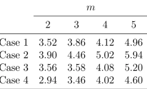
presented. In addition, table 2 includes the empirical sizes of the well-known BDS

3_{The betas have been demeaned.}

4_{This sample size was chosen as representative of the actual sample size for the empirical results}

test proposed by Brock, Dechert, Scheinkman and LeBaron (1996), for testing the hypothesis that the standardized residuals are iid. To calculate the BDS, we must specify the values of two parameters, the embedding dimension,m, and the distance parameter, "=s, where s denotes the sample standard deviation. Brock, Hsieh and LeBaron (1991), suggest that " should take values in the interval[0:5;1:5], and that

m should be in line with the number of observations. Given the selected sample sizeT = 1000, and the fact that" a¤ects the power of the test, the reported results correspond to m = 2;3;4;5 and "=s= 1.

The results may be summarized as follows:

(i) The ML estimators of all the parameters in SFMT-AR work su¢ ciently well for all the parameter con…gurations under study, including those in which the autore-gressive coe¢ cient for _{f tg}is near unity (case 3). The average biases and standard deviations decrease as the sample size increases and the biases are su¢ ciently small even for T = 250. For example, for T = 500; the bias ofb is equal to -0.041, -0.062, -0.055 and -0.03 for cases 1, 2, 3 and 4, respectively. When the sample size increases to T = 1000; the corresponding bias decreases, in absolute terms, to -0.015, -0.015, -0.008 and -0.005, respectively.

(ii) The t-statistics corresponding to the parameters a; 2

u and 2" are properly

sized, for all the four cases under consideration, even for sample sizes as small as

T = 250: The t-statistics for b = ; appear to be over-sized, even for T = 1000;

in the cases of strongly persistent betas, namely cases 2 and 3. Size distortions in both directions are reported for the t-statistics of b= for all the four cases under consideration except for case 2. This means that testing the hypothesis b= is, in general problematic unless _{f tg} exhibits strong (but not extremely strong) persis-tence. This is attributed to the small rate of convergence in the case of very high and very low persistence. For example, in case 3, when the number of observations increases to T = 4000, the size distortions become much smaller.5

5_{The empirical sizes for testing the hypotheses b = and b = become 3.88 and 8.06,}

(iii) The empirical sizes of the BDS tests (reported in table 2), are in general close to their nominal values, especially for m = 5 and T = 1000, for all the cases under consideration.

3

Empirical Results

The empirical analysis of this paper is based on the S&P500 sector data (see, for example, DeMiguel, Garlappi and Uppal (2007), and Anderson, Brooks and Katsaris (2010) among others for similar datasets). We follow the Global Industry Classi-…cation Standard (GICS), designed and maintained by Standard & Poor’s (S&P) and Morgan Stanley Capital International (MSCI), which consists of the following 10 sectors: 1: Consumer Discretionary, 2: Consumer Staples, 3: Energy, 4: Fi-nancials, 5: Healthcare, 6: Industrials, 7: Information Technology, 8: Materials, 9: Telecommunications and 10: Utilities. The dataset consists of weekly returns on the value-weighted indices of the aforementioned sectors, the returns on the S&P 500 Index (used as an approximation of the single factor, Mt) and the return of

the 90-day T-bill, which is used as a proxy for the risk-free rate6_{. All the series}

are obtained from Bloomberg (except for the risk-free rate which was obtained from Ken French’s Data Library website) and cover the period 22/9/1989 - 28/12/2012.

3.1

In-sample Comparisons

Using this dataset, we estimate the SFMT, SFMT-GARCH, SFMT-B- GARCH and SFMT-AR models. As already mentioned, SFMT is the simple homoscedastic model

rt= + Mt+ t; in which f tg is assumed to be a niid process with zero mean

and …nite variance-covariance matrix, v = diagf 2v1; :::; 2

vng: SFMT-GARCH is

de…ned as follows:

6_{Following the tradition of the empirical literature (see for example, Fama and French 1996, Ng,}

Engle and Rothschild 1992) we employ excess rather than simple returns in the empirical analysis of this section. To avoid additional notational burden, we shall refrain from changing the relevant notation, which means that from now onri;t will denote the excess return on asseti.

rt= + Mt+zt; (13)

where ztis a vector whose elements are zi;t = p

hi;t"i;t; where hi;t = ci + i"2i;t 1 +

ihi;t 1; i = 1; :::; n and f"i;tg is NIID(0,1). Note that since Mt is assumed to be

the only source of correlation among the elements of rt, the conditional covariance

matrix, z

t;t 1;of zt is diagonal. Then, tjt 1;(SF M T GARCH) = zt;t 1 + 2m 0:

SFMT-B-GARCH is de…ned as follows:

ri;t Mt = i m + ui;t um;t = i +ui_t; i= 1; :::;10 where ui_t=ztH 1=2 i;t

and zt is a 2-dimensional IID process with zero mean and the identity covariance

matrix. We employ the constant correlation model7 of Bollerslev (1990) to parame-terize H1_i;t=2, and therefore,

Hi;t = 2 6 4cii+ ii" 2 i;t 1+ iihii;t 1 im p hii;t p hmm;t im p hii;t p hmm;t cmm+ mm"2m;t 1+ mmhmm;t 1 3 7 5:

Note that, under SFMT-B-GARCH, in contrast to our approach up to now, we also model explicitly the conditional variance of Mt: Under the assumptions thus far, we

may write ri;t =ai;t+bi;tMt+ui;t; where ai;t = i bi;t m; bi;t = him;t

hmm;t and ui;t is a

zero-mean process with variance equal to and ~hii;t=hii;t h2

im;t

hmm;t. As a consequence,

the conditional covariance matrix of the 10 sectors is given by:

tjt 1;(SF M T B GARCH)=btb0thmm;t+ ut;t 1;

where b0

t = [b1;t; b2;t; : : : ; b10;t] 0

and u

t;t 1 = diag ~h11;t; : : : ;~h1010;t . Note that the

time-varying betas can be re-written as: bi;t = him;t hmm;t = _im p hii;t p hmm;t ; i= 1; :::;10:

The estimation results for SFMT, GARCH, B-GARCH and SFMT-AR are reported in Tables 3, 4, 5 and 6, respectively. These tables include also the results from the application of the BDS test on the standardized residuals of the aforementioned models.8 _{An additional standard test for the presence of}

second-order e¤ects in the standardized residuals is also reported.

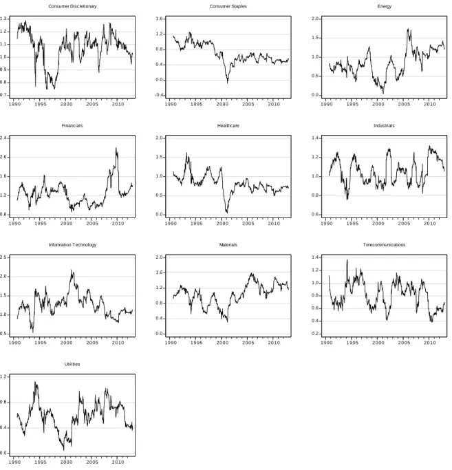
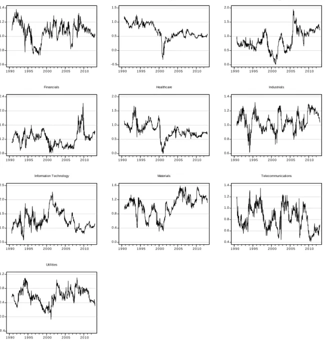
Additional diagnostic tests, aiming at assessing the degree of time variation in the beta coe¢ cient, are reported in Figures 1 and 2 (Appendix B). These Figures contain rolling estimates of the beta coe¢ cient for all the ten sectors under consideration and for both models which assume a time-invariant beta, namely, for SFMT and SFMT-GARCH9. The overall results may be summarized as follows:

(i) In the context of the constant-beta homoscedastic SFMT model, the OLS estimates of beta from the ten sectors under consideration are quite disperse, ranging from 0.58 for the Utilities sector to 1.35 for the Financials one. However, there is strong evidence that this model is seriously misspeci…ed. For all the ten sectors, the aforementioned test for higher-order temporal dependence rejects the hypothesis that the standardized residuals form an independent sequence. Furthermore, the rolling OLS estimates of beta, reported in Figure 1, leave no doubt that the constant beta assumption does not enjoy empirical support. Indeed, in some cases the time variation of betas is impressive. For example, in the case of Consumer Staples sector, the estimates of beta range from -0.08 to 1.26 for the estimation periods 9-March 2001 and 29-October 1993, respectively.

(ii) As far as SFMT-GARCH is concerned, the ML estimates of its parameters are broadly consistent with the ones reported in the empirical literature, that is, the

8_{The reported results correspond to the case where "=s = 1and m= 3: Results for the cases} m= 2;4and5 (not reported) provide similar conclusions.

sum of the GARCH coe¢ cients _bi +bi is close to unity withbi being much larger

than bi. As expected, SFMT-GARCH performs far better than SFMT in terms of

in-sample performance criteria. Speci…cally, the standardized residuals of SFMT-GARCH appear to be independent for all the sectors under consideration, with the possible exceptions of Financials and Industrials. However, additional misspeci…ca-tion testing reveals that SFMT-GARCH is not empirically adequate. Speci…cally, the rolling ML estimates of beta in the context of SFMT-GARCH, reported in Figure 3, suggest that substantial (or even massive) parameter instability is still present. This in turn implies that SFMT-GARCH does not capture adequately the exact form of CH exhibited by the returns generating process. In other words, the time variation of betas may be interpreted as evidence of important discrepancy between the type of second-order e¤ects that truly characterize _frtg and those implied by

SFMT-GARCH.

(iii) The SFMT-B-GARCH also performs far better than SFMT in terms of in-sample performance criteria. However, the standardized residuals of SFMT-B-GARCH as opposed to those of SFMT-SFMT-B-GARCH, do not appear to be temporally independent in general. On the other hand, SFMT-B-GARCH captures, to some extent, the time variation of betas. These results show that the two GARCH models produce di¤erent sets of empirical results with neither of them being clearly superior to the other.

(iv) Turning to the SFMT-AR model, the …rst thing to observe is the emergence of two distinct patterns of persistence for the beta process. Speci…cally, there is one group of sectors (HP) consisting of Consumer Staples, Energy, Healthcare, In-formation Technology and Materials for which the beta is highly persistent. The rest …ve sectors form another subset (LP) for which the beta persistence is low (Consumer Discretionary, Financials, Industrials) or even zero (Telecommunica-tions, Utilities). As a result, HP exhibits strong second-order e¤ects as opposed to LP in which dynamic heteroscedasticity is weak, if present at all. This varying

degree of second-order e¤ects within the set of returns series under consideration im-plied by SFMT-AR is in sharp contrast with the uniformity of volatility persistence impinged upon the aforementioned series by SFMT-GARCH. As far as empirical adequacy is concerned, SFMT-AR does not succeed in delivering independent stan-dardized residuals in any of the ten series under study. This means that SFMT-AR does not fully capture the second-order e¤ects of _frtg: Another interesting question

would be to compare the time-variation of betas produced by SFMT-AR to that of SFMT-B-GARCH. Table 7 reports the correlations between the conditional betas from the two approaches, for each sector. These correlations suggest that betas di¤er between the two approaches and sometimes, this di¤erence is substantial (see, for example, the negative correlation in the case of the Telecommunication sector betas). The overall assessment of the results on SFMT-GARCH, SFMT-B-GARCH and SFMT-AR seem to suggest that neither of these models provide an adequate characterization of the second-order dynamics of the returns generating process. As a result, the relevant question becomes that of which of these models comes closer to approximating the true CH exhibited by _frtg:This question may also be stated

in the form: which of these models fares better in forecasting the next period’s covariance matrix of returns? This question is addressed in the next sub-section.

(v) The estimated SFMT-GARCH conditional variance process di¤ers radically from the SFMT-AR one, even in the cases where SFMT-AR delivers highly persistent processes. Table 8 reports the correlation coe¢ cients between the two conditional variance processes, for the ten sectors under consideration. These coe¢ cients are, in general, close to zero or even negative. More speci…cally, the estimates of the correlation coe¢ cient range from -0.561 to 0.613 for Information Technology and Financials, respectively. It is interesting to note the strong negative correlation between the SFMT-GARCH and SFMT-AR conditional variance processes for the Information Technology sector, which is characterized by the most persistent beta process among all the sectors under consideration. These results imply that in spite

of the fact that both SFMT-GARCH and SFMT-AR entail second-order, persistent e¤ects, the exact types of CH implied by these models are quite di¤erent.

3.2

Out-of-Sample Comparisons

To take into account the possibility that, eitherMtis not a good proxy of the market

portfolio, or that this is not the only factor accounting for the observed correlations between ri;t and rj;t; we also consider an additional model, hereafter referred to as

SFMT-MGARCH, in which the errors of the ten factor models are jointly modelled as a multivariate GARCH process. More speci…cally, de…ne r0_t to be the (10 1)

time-series vector [r1;t; r2;t; : : : ; r10;t] 0

. Consider a system of 10 conditional mean equations rt = a+bMt+ut; where ut = ztH

1=2

t and zt is a 10-dimensional IID

process with zero mean and the identity covariance matrix. Again, we employ the constant correlation model to parametrize Ht, and therefore,

hij;t= cii+ ii"2i;t 1+ iihii;t 1; i=j ij p hii;t p hjj;t; i6=j ; i; j = 1; :::;10: Then, tjt 1;(SF M T M GARCH)=bb0 2m+Ht:

The out-of-sample comparisons are carried out as follows: First, we select an ini-tial sample, referred to as the estimation sample, for which all the competing mod-els, namely SFMT, GARCH, B-GARCH, MGARCH, SFMT-AR, are estimated. Although various alternative estimation samples were tried and produced similar results, our reported results refer to the period 22/9/1989 -30/12/2005. Second, using the estimated parameters, we produce one-step ahead forecasts of the conditional covariance matrix, tjt 1;for each of the aforementioned

models for the period 6/1/2006 - 28/12/2012, thus obtaining 365 one-week ahead forecasts. To remind the reader, the conditional covariance matrices implied by SFMT, SFMT-GARCH, SFMT-B-GARCH, SFMT-MGARCH and SFMT-AR are

given by: tjt 1;(SF M T) = v + 2m 0; tjt 1;(SF M T GARCH) = zt;t 1+ 2 m 0; tjt 1;(SF M T BGARCH) = t;tu 1+hmm;tbtb0t; tjt 1;(SF M T M GARCH) = Ht+ 2mbb0; tjt 1;(SF M T AR) = 2m "+ u+ 2m + t=t 1 + t=t 1 0 :

Using these matrices we calculate the global minimum variance portfolios together with the corresponding realized portfolio returns. The reason for selecting the global minimum variance portfolio is to minimize the estimation errors relating to the estimation of the expected returns. This procedure results in 365 out-of-sample realized portfolio returns for each model. For comparison purposes, apart from the SFMT, SFMT-GARCH, SFMT-B-GARCH, SFMT-MGARCH and SFMT-AR portfolios, we also calculate the portfolio returns that correspond to the case in which in btjt 1 is the sample covariance matrix (SCM) and also for the case in which the

portfolio is formed according to the naive 1/n (1=N) strategy. To assess the out-of-sample performance of each strategy, we employ the following three criteria: (i) the out-of-sample Sharpe ratio (SR = i

i), (ii) the Certainty-Equivalent Return

(CEQ = _{i 2} i), where is the risk-aversion coe¢ cient, and (iii) the

out-of-sample Treynor ratio (T R = i

i), where i is the portfolio’s beta relative to the

market portfolio. Following common practice, the CEQ return is de…ned to be the risk-free rate that an investor is willing to accept in order to be indi¤erent between choosing this riskless return and the return of the strategy. CEQ is calculated for various values of ; with largely similar results (the reported ones correspond to

= 1).

The results, reported in Table 9, may be summarized as follows:

performance criteria mentioned above, although di¤erences are marginal. For ex-ample, the SR of SFMT-AR is greater than that of SFMT-GARCH, SFMT-B-GARCH, SFMT-MSFMT-B-GARCH, SFMT, SCM and 1=N by 6.24%, 105.50%, 5.00%, 11.77%, 14.58% and 456.48%, respectively. It is worth noting that all the statistical methods dominate the naive 1=N strategy by a wide margin. This piece of evidence runs counter to the view expressed in De Miquel, Garlappi and Uppal (2007) ac-cording to which no statistical method for forecasting the returns covariance matrix o¤ers signi…cant diversi…cation gains over the 1=N strategy.

(ii) The SFMT-GARCH strategy comes second to SFMT-AR, o¤ering some mi-nor gains over the homoscedastic SFMT and the non-parametric SCM ones, but very signi…cant gains over the naive 1=N strategy. It is also worth noting the excep-tionally poor performance of SFMT-B-GARCH, which appears to be superior only to that of 1=N strategy.

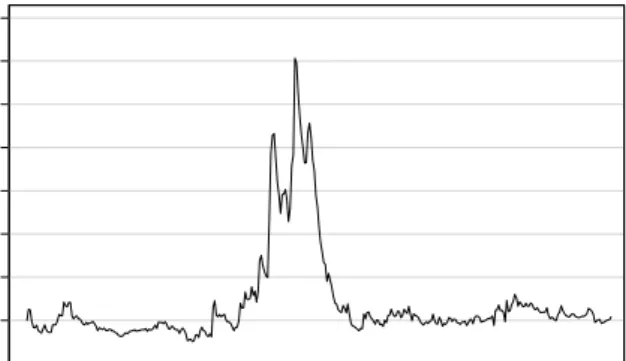
Finally, it would be interesting to examine the di¤erences between the fore-casted covariance matrices produced by the two best performing models, namely SFMT-AR and SFMT-GARCH. To this end, we de…ne a distance, dAR GARCH

be-tween tjt 1;(SF M T AR) and tjt 1;(SF M T GARCH) and examine how this di¤erence

has evolved over the forecast period under consideration. Foerstner and Moonen (1999) de…ne the distance between two symmetric semi-positive de…nite matrices as the sum of the squared logarithms of the properly de…ned eigenvalues, that is:

dAR GARCH = v u u t n X i=1 ln( i( tjt 1;(SF M T AR); tjt 1;(SF M T GARCH)))2

with the eigenvalues i( tjt 1;(SF M T AR); tjt 1;(SF M T GARCH)); i= 1; :::; nobtained

from the solution of_j tjt 1;(SF M T AR) tjt 1;(SF M T GARCH)j= 0. The time

evo-lution of dAR GARCH, presented in Figure 3 (Appendix B), suggests …rst that this

distance ranges from 1.08 on 25/01/2008 to 4.05 on 19/12/2008. It also suggests that

return-ing to more normal levels after the …rst quarter of 2009. We obtain similar results when we use the Frobenius norm to calculate the distance, between tjt 1;(SF M T AR)

and tjt 1;(SF M T GARCH);(see Figure 4 in Appendix B). Speci…cally, the results show

a signi…cant increase of the di¤erence between the conditional covariance matrices produced by SFMT-AR and SFMT-GARCH during the one-year period that starts approximately at the bankruptcy date of Lehman Brothers (9/15/2008). Motivated by this observation, we examine the out-of sample performance of the models under consideration for the period 9/2008 - 8/2009. Because the annualized returns are negative for this period, the SR and TR statistics are not appropriate measures for comparing the models.10

Table 10 presents the results concerning CEQ, as well as the annualized returns and risk for each model. We observe that the strategy implied by SF M T AR

combines the smallest (in absolute values) negative return with the lowest annualized risk. This results to a CEQ which is at least 11,85% higher than the corresponding value of the second best model (which, in terms of CEQ, is SF M T M GARCH). Note that the calculation of CEQ in Table 10 retains the value of equal to1. On the other hand, it is worth noting that during the period that followed the bankruptcy of Lehman Brothers, the risk aversion increased. This fact in combination with the best performance of SF M T ARin terms of both annualized return and risk, implies that the di¤erence between the CEQ of SF M T AR and the CEQ of the second best model is actually bigger for this period.11

10_{For example, if two models produce comparable (in magnitude) annualized returns but the}

annualized standard deviation (beta) of the …rst is larger, the Sharpe (Treynor) ratio of the …rst model becomes smaller (less negative) than that of the second one.

11_{A natural extension of our empirical analysis would be to examine whether the combination of}

autoregressive betas with GARCH errors would yield better out of sample performance. To this end we repeated the out of sample study for the speci…c model (SF M T ARG). The results, however, were not satisfactory. Speci…cally, SF M T ARG outperforms onlySF M T B GARCH and the equally weighted portfolio.

4 Conclusions

This paper has examined the in-sample and out-of-sample performance of several variants of the single factor model for stock returns. Attention was focused mainly on SFMT-GARCH in the context of which the idiosyncratic risk is conditionally heteroscedastic and SFMT-AR which assumes an autoregressive structure for the systematic risk and homoscedasticity for the non-systematic one. A large part of the paper dealt with the theoretical properties as well as the estimation issues of SFMT-AR. It was proved that SFMT-AR is capable of reproducing the most important stylized facts of individual stock returns, namely conditional heteroscedasticity and leptokurtosis. Interestingly enough, this result continues to hold even in the case in which the stochastic process generating the “unanticipated changes of the factor” is independent. The empirical results showed that none of the factor models under examination is fully empirically adequate, in terms of in-sample criteria. For exam-ple, SFMT-GARCH still su¤ers from substantial beta variation whereas SFMT-AR does not account fully for conditional heteroscedasticity.

However, these models o¤er signi…cant gains for forecasting next period’s co-variance matrix of returns over the homoscedastic SFMT and the non-parametric method of forecasting second moments via their sample analogues. Moreover, these gains are maximized relative to the naive (1/N) allocation strategy, which in some recent studies was found to deliver the greatest portfolio diversi…cation gains among a set of strategies that include various statistical methods (see, e.g. De Miguel et. al. 2007). Among the four conditionally heteroscedastic models under considera-tion, namely SFMT-AR, SFMT-GARCH, SFMT-B-GARCH and SFMT-MGARCH, the former was found to exhibit systematically the best out-of-sample performance, closely followed by SFMT-GARCH.

References

Andersen, Torben G., Tim Bollerslev, Francis X. Diebold, and Paul Labys, 2003, Modeling and Forecasting Realized Volatility, Econometrica 71, 579-625.

Andersen, Torben G., Tim Bollerslev, Francis X. Diebold and Jin Wu, 2005, A Framework for Exploring the Macroeconomic Determinants of Systematic Risk,

American Economic Review 95, 2, 398-404.

Anderson K., C. Brooks, A. Katsaris, 2010, Speculative bubbles in the S&P 500: Was the tech bubble con…ned to the tech sector?, Journal of Empirical Finance 17, 345–361.

Ang, Andrew, and Joseph Chen, 2007, CAPM over the long run: 1926-2001,Journal of Empirical Finance 14, 1-40.

Arditti, Fred D., 1967 Risk and the Required Return on Equity,Journal of Finance

22, 19-36.

Avramov, Doron, and Tarun Chordia, 2006, Asset Pricing Models and Financial Market Anomalies, Review of Financial Studies 19, 1001-1040.

Barndor¤-Nielsen, Ole E., and Neil Shephard, 1998, Aggregation and model con-struction for volatility models, Centre for Analytical Finance, University of Aarhus, Working Paper Series No. 10.

Bali, Turan G., Hengyong Mo and Yi Tang, 2008, The role of autoregressive con-ditional skewness and kurtosis in the estimation of concon-ditional VaR, Journal of Banking and Finance 32, 269-282.

Beja, Avraham, 1972, On Systematic and Unsystematic Components of Financial Risk, Journal of Finance 27, 37-45.

Berk, Jonathan B., Richard C. Green and Vasant Naik, 1999, Optimal Investment, Growth Options, and Security Returns, Journal of Finance 54, 1553-1607.

Blattberg, Robert C., and Nicholas J. Gonedes, 1974, A Comparison of the Stable and Student Distributions as Statistical Models for Asset Prices,Journal ofBusiness

47, 244-280.

Blume, Marshall E., 1971, On the assessment of risk, Journal of Finance 26, 1-10. — — — — — , 1975, Betas and Their Regression Tendencies, Journal of Finance 30, 785-795.

Bollerslev, Tim, Robert F. Engle and Je¤rey M. Wooldridge, 1988, A Capital Asset Pricing Model with Time Varying Covariances, Journal of Political Economy 96, 116-131.

Bos, Theodore, and Paul Newbold, 1984, An emprical investigation of the possibility of stochastic systematic risk in the market model, Journal of Business 57, 35-41. Bos, Theodore, and Thomas A. Fetherston, 1992, Market model nonstationarity in the Korean Stock Market, Paci…c Basin Capital Market Research, 3.

— — — — — — — — — — , 1995, Nonstationarity of the market model, outliers, and the choice of market rate of return, in Theodore Bos, Thomas A. Fetherston, eds.:

Advances in Paci…c Basin Financial Markets, Vol. 1 (JAI Press, Greenwich, CT). Brock, W.A., Dechert, W.D., Scheinkman, J.A., LeBaron, B., 1996, A test for inde-pendence based on the correlation dimension. Econometrics Review 15, 197–235. Brock, William A., Hsieh, David A. and LeBaron Blake, 1991, Nonlinear dynamics, chaos and instability. The MIT Press, Cambridge, Massachusetts.

Castanias, Richard P. II, 1979, Macroinformation and the Variability of Stock Mar-ket Prices, Journal of Finance 34, 439-450.

Clark, Peter K., 1973, A Subordinated Stochastic Process Model with Finite Vari-ance for Speculative Prices, Econometrica 41, 135-155.

— — — — –, 1987, The Cyclical Component of U.S. Economic Activity, Quarterly Journal of Economics 102, 797-814.

Collins, Daniel W., Johannes Ledolter and Judy Rayburn, 1987, Some Further Ev-idence on the Stochastic Properties of Systematic Risk, Journal of Business 60, 425-448.

DeMiguel V, Garlappi L, Uppal R., 2009, Optimal versus naive diversi…cation: How ine¢ cient is the 1/N portfolio strategy? Review of Financial Studies. 22:1915–53 Fabozzi, Frank J., and Jack Clark Francis, 1977, Stability Tests for Alphas and Betas Over Bull and Bear Market Conditions, Journal of Finance 32, 1093-1099. Fa¤, Robert W., John H. H. Lee and Tim R. L. Fry, 1992. Time stationarity of sys-tematic risk: some Australian evidence. Journal of Business Finance & Accounting, 19, 253-270.

— — — — — — — — — — — — –, 1978. Beta as a random coe¢ cient. Journal of Fi-nancial and Quantitative Analysis, 13, 101-116.

Fama, Eugene F., 1965. The behavior of stock-market prices. Journal of Business, 38, 34-105.

— — — — –, 1968. Risk, Return and Equilibrium: Some Clarifying Comments. Jour-nal of Finance, 23, 29-40.

Fama, Eugene F., and Kenneth R. French, 1988. Permanent and Temporary Com-ponents of Stock Prices. Journal of Political Economy, 96, 246-273.

— — — — — — — — — — — — — — — –, 1996, Multifactor explanations of asset pricing anomalies, Journal of Finance 51, 55-84.

Fisher, Lawrence, and Jules H. Kamin, 1985, Forecasting Systematic Risk: Esti-mates of ‘Raw’Beta That Take Into Account the Tendency of Beta to Change and

the Heteroscedasticity of Residual Returns, Journal of Financial and Quantitative Analysis 20, 127-149.

Förstner, Wolfgang and Moonen Boudewijn, 1999, A metric for covariance matrices. Technical report, Dept. of Geodesy and Geoinformatics, Stuttgart University. Granger, Clive W. J., 1968, Some Aspects of the Random walk Model of Stock Market Prices, International Economic Review 9, 253-257.

Hagerman, Robert L., 1978, More Evidence on the Distribution of Security Returns,

Journal of Finance 33, 1213-1221.

Harvey, Campbell R., 1989, Forecasts of Economic Growth from the Bond and Stock Markets, Financial Analysts Journal 45, 38-45.

Harvey, Campbell R., and Akhtar Siddique, 1999, Autoregressive Conditional Skew-ness, Journal of Financial and Quantitative Analysis 34, 465-487.

— — — — — — — — — — — , 2000a, Conditional Skewness in Asset Pricing Tests, Jour-nal of Finance 55, 1263-1295.

— — — — — — — — — — — , 2000b, Time Varying Conditional Skewness and the Mar-ket Risk Premium, Research in Banking and Finance 1, 25-58.

Hsu, Der-Ann, Robert B. Miller and Dean W. Wichern, 1974, On the stable Paretian behavior of stock-market prices,Journal of the American Statistical Association 69, 108-113.

Jostova, Gergana, and Alexander Philipov, 2005, Bayesian Analysis of Stochastic Betas, Journal of Financial and Quantitative Analysis 40, 747-778.

Kendall, Maurice G., 1953, The Analysis of Economic Time-Series-Part I: Prices,

Kim, Myung J., Charles R. Nelson and Richard Startz, 1991, Mean Reversion in Stock Prices? A Reappraisal of the Empirical Evidence, Review of Economic Studies

58, 515-528.

Kim, Chang-Jin., and Charles R. Nelson, 1999, State-Space Models with Regime Switching, MIT Press, London, England and Cambridge, Massachusetts.

Kon, Stanley J., 1984, Models of Stock Returns–A Comparison, Journal of Finance

39, 147-165.

Kon, Stanley J., and Frank C. Jen, 1978, Estimation of Time-Varying Systematic Risk and Performance for Mutual Fund Portfolios: An Application of Switching Regression, Journal of Finance 33, 457-475.

Kraus, Alan, and Robert H. Litzenberger, 1976, Skewness Preference and the Valu-ation of Risk Assets, Journal of Finance 31, 1085-1100.

Levenberg K., 1944, A method for the solution of certain problems in least squares,

Quarterly of Applied Mathematics, Vol. 2, pp. 164-168.

Lim, Kian-Guan., 1989, A New Test of the Three-Moment Capital Asset Pricing Model, Journal of Financial and Quantitative Analysis 24, 205-216.

Lo, Andrew W., and A. Craig MacKinlay, 1988, Stock Market Prices do not Follow Random Walks: Evidence from a Simple Speci…cation Test, Review of Financial Studies 1, 41-66.

Madan, Dilip B., and Eugene Seneta, 1990, The Variance Gamma (V.G.) Model for Share Market Returns, Journal of Business 63, 511-524.

Mandelbrot, Benoit, 1963, The Variation of Certain Speculative Prices, Journal of Business 36, 394-419.

Mandelbrot, Benoit, and Howard M. Taylor, 1967, On the Distribution of Stock Price Di¤erences, Operations Research 15, 1057-1062.

Mankiw, N. Gregory, David Romer and Matthew D. Shapiro, 1991, Stock Market Forecastability and Volatility: A Statistical Appraisal, Review of Economic Studies

58, 455-477.

McQueen, Grant, 1992, Long-Horizon Mean-Reverting Stock Prices Revisited, Jour-nal of Financial and Quantitative AJour-nalysis 27, 1-18.

Mergner, Sascha and Jan Bulla, 2008, Time-varying Beta Risk of Pan-European In-dustry Portfolios: A Comparison of Alternative Modeling Techniques,The European Journal of Finance, vol. 14, no. 8, pp. 771–802.

Merton, R. C, 1973, “An Intertemporal Capital Asset Pricing Model.”Econometrica

41 (5): 867–87.

Miller, Merton, and Myron Scholes, 1972, Rates of return in relation to risk: A reexamination of some recent …ndings, in Michael Jensen, ed.: Studies in the theory of capital markets (Praeger, New York).

Ng, V.K., R.F. Engle and M. Rothschild, 1992, “A Multi-Dynamic-Factor Model for Stock Returns,”Journal of Econometrics, 52, 245-266.

O¢ cer, Robert R., 1972, The Distribution of Stock Returns,Journal of the American Statistical Association 67, 807-812.

Ohlson, James, and Barr Rosenberg, 1982, Systematic Risk of the CRSP Equal-Weighted Common Stock Index: A History Estimated by Stochastic-Parameter Re-gression, Journal of Business 55, 121-145.

Osborne, Matthew F. M., 1959, Brownian Motion in the Stock Market, Operations Research 7, 145-173.

Pagan, A., 1980, “Some Identi…cation and Estimation Results for Regression Models with Stochastically Varying Coe¢ cients”, Journal of Econometrics 13, pp.341-63.

Peligrad, Magda, and Sergey Utev, 2005, A new maximal inequality and invariance principle for stationary sequences, The Annals of Probability 33, 798-815.

Petkova, Ralitsa, and Lu Zhang, 2005, Is value riskier than growth? Journal of Financial Economics 78, 187-202.

Poterba, James M., and Lawrence H. Summers, 1988, Mean reversion in stock prices : Evidence and Implications, Journal of Financial Economics 22, 27-59.

Praetz, Peter D., 1972, The Distribution of Share Price Changes,Journal of Business

45, 49-55.

Richardson, Matthew, 1989, Predictability of stock returns: statistical theory and evidence. Ph.D. Thesis, Stanford University, Graduate School of Business.

Richardson, Matthew, and and James H. Stock, 1989, Drawing inferences from statistics based on multiyear asset returns,Journal of Financial Economics 25, 323-348.

Ross, Stephen, 1976, “The arbitrage theory of capital asset pricing”. Journal of Economic Theory 13 (3): 341–360.

Schwartz, Robert A., and David K. Whitcomb, 1977, The Time-Variance Relation-ship: Evidence on Autocorrelation in Common Stock Returns, Journal of Finance

32, 41-55.

Shanken, J., 1990, Intertemporal asset pricing: an empirical investigation, Journal of Econometrics 45, 99–120.

Stout, William F., 1974. Almost Sure Convergence (Academic Press, New York, NY).

Sunder, Shyam, 1980, Stationarity of Market Risk: Random Coe¢ cients Tests for Individual Stocks, Journal of Finance 35, 883-896.

Upton, David E., and Donald S. Shannon, 1979, The Stable Paretian Distribution, Subordinated Stochastic Processes, and Asymptotic Lognormality: An Empirical Investigation, Journal of Finance 34, 1031-1039.

APPENDIX A

Proof of Theorem 1:

(a) For notational simplicity, we drop the subscript i. First note that

(V ar(rt))2= 2+ 2 2m+ 2 2 ₊ 2 u 2 = 4_u+ 4 4 + 4 4_m+ 4_m 4 + +2 2 2_m 4 + 2 _u2 2 + 2 2_m 2_u+ 2 4_m 2 + 2_m 2_u 2 + 2 2 2_m 2(14)

Moreover, for the fourth central moment of rt we have

E (rt E[rt]) 4 = E ( wt+ t( +wt) +ut) 4 = E u4_t + 4 4_t +w4_t 4+w_t4 4_t + 6 2u2_t 2_t + 6 2w2_t 4_t +6u2_tw2_t 2+ 6u2_tw_t2 _t2+ 6w4_t 2 2_t + 6 2w_t2 2 2_t = 3 4_u+ 4 4 + 4 4_m+ 4 4_m + 2 2 2_u 2 + 3 2 2_m 4 + 2 2_u 2_m+ 2 2_{u m}2 + 3 2 2 4_m+ 2 2 2 2_m = 3V ar2(rt) + 12 2 2m 4 + 2 2 4_m , (15)

where we have used the fact that for the Gaussian distributions, the third moment is zero and fourth moment equals to three times the square of the second. Hence, the kurtosis coe¢ cient of the unconditional distribution of stock returns is given by

Kurt(rt) = E (rt E[rt])4 V ar2_(r t) = 3 + 12 2 2 m 4 + 2 2 4 m V ar2_(r t) : (16)

APPENDIX B

0 .7 0 .8 0 .9 1 .0 1 .1 1 .2 1 .3 1 9 9 0 1 9 9 5 2 0 0 0 2 0 0 5 2 0 1 0 Consumer Discretionary - 0 .4 0 .0 0 .4 0 .8 1 .2 1 .6 1 9 9 0 1 9 9 5 2 0 0 0 2 0 0 5 2 0 1 0 Consumer Staples 0 .0 0 .5 1 .0 1 .5 2 .0 1 9 9 0 1 9 9 5 2 0 0 0 2 0 0 5 2 0 1 0 Energy 0 .8 1 .2 1 .6 2 .0 2 .4 1 9 9 0 1 9 9 5 2 0 0 0 2 0 0 5 2 0 1 0 Financials 0 .0 0 .5 1 .0 1 .5 2 .0 1 9 9 0 1 9 9 5 2 0 0 0 2 0 0 5 2 0 1 0 Healthcare 0 .6 0 .8 1 .0 1 .2 1 .4 1 9 9 0 1 9 9 5 2 0 0 0 2 0 0 5 2 0 1 0 Industrials 0 .5 1 .0 1 .5 2 .0 2 .5 1 9 9 0 1 9 9 5 2 0 0 0 2 0 0 5 2 0 1 0 Information Technology 0 .0 0 .4 0 .8 1 .2 1 .6 2 .0 1 9 9 0 1 9 9 5 2 0 0 0 2 0 0 5 2 0 1 0 Materials 0 .2 0 .4 0 .6 0 .8 1 .0 1 .2 1 .4 1 9 9 0 1 9 9 5 2 0 0 0 2 0 0 5 2 0 1 0 Telecommunications 0 .0 0 .4 0 .8 1 .2 1 9 9 0 1 9 9 5 2 0 0 0 2 0 0 5 2 0 1 0 Utilities

0 .6 0 .8 1 .0 1 .2 1 .4 1 9 9 0 1 9 9 5 2 0 0 0 2 0 0 5 2 0 1 0 Consumer Discretionary - 0 .5 0 .0 0 .5 1 .0 1 .5 1 9 9 0 1 9 9 5 2 0 0 0 2 0 0 5 2 0 1 0 Consumer Staples 0 .0 0 .5 1 .0 1 .5 2 .0 1 9 9 0 1 9 9 5 2 0 0 0 2 0 0 5 2 0 1 0 Energy 0 .8 1 .2 1 .6 2 .0 2 .4 1 9 9 0 1 9 9 5 2 0 0 0 2 0 0 5 2 0 1 0 Financials 0 .0 0 .5 1 .0 1 .5 2 .0 1 9 9 0 1 9 9 5 2 0 0 0 2 0 0 5 2 0 1 0 Healthcare 0 .6 0 .8 1 .0 1 .2 1 .4 1 9 9 0 1 9 9 5 2 0 0 0 2 0 0 5 2 0 1 0 Industrials 0 .5 1 .0 1 .5 2 .0 2 .5 1 9 9 0 1 9 9 5 2 0 0 0 2 0 0 5 2 0 1 0 Information Technology 0 .0 0 .4 0 .8 1 .2 1 .6 1 9 9 0 1 9 9 5 2 0 0 0 2 0 0 5 2 0 1 0 Materials 0 .4 0 .6 0 .8 1 .0 1 .2 1 .4 1 9 9 0 1 9 9 5 2 0 0 0 2 0 0 5 2 0 1 0 Telecommunications - 0 .4 0 .0 0 .4 0 .8 1 .2 1 9 9 0 1 9 9 5 2 0 0 0 2 0 0 5 2 0 1 0 Utilities

1.0 1.5 2.0 2.5 3.0 3.5 4.0 4.5 2006 2007 2008 2009 2010 2011 2012 SFMT-AR vs SFMT-GARCH

Figure 3: The time evolution ofdAR GARCH:

.000 .001 .002 .003 .004 .005 .006 .007 .008 2006 2007 2008 2009 2010 2011 2012 SFMT-AR vs SFMT-GARCH

Figure 4: The time evolution of the di¤erence in the covariance matrices, using the Frobenius norm.

Table 1: Monte-Carlo results Panel A: Persistent betas

ln( 2 u) ln( 2) Case 1 bias 0:00 0:01 0:62 0:39 1:49 std 0:00 0:59 0:53 4:90 0:49 kurt 3:02 3:00 3:00 3:80 12:84 skew 0:02 0:01 0:08 0:41 1:97 size(%) 4:54 7:26 5:62 5:84 5:14 Case 3 bias 0:00 0:12 0:52 7:57 0:84 std 0:00 1:66 0:47 4:93 0:20 kurt 3:00 2:96 2:92 4:75 822:11 skew 0:01 0:04 0:13 0:20 22:09 size(%) 5:30 16:46 4:66 4:58 0:84

Panel B: Non-persistent betas

ln( 2 u) ln( 2) Case 1 bias 0:00 0:01 0:38 5:01 1:50 std 0:00 0:37 0:63 2:75 1:67 kurt 3:01 2:96 2:95 8:37 4:08 skew 0:03 0:02 0:07 1:31 0:41 size(%) 4:48 5:06 4:84 4:02 7:08 Case 4 bias 0:00 0:04 0:20 23:70 0:48 std 0:01 0:49 0:61 6:44 3:19 kurt 3:06 2:94 3:00 18:72 3:34 skew 0:01 0:01 0:01 2:87 0:10 size(%) 5:46 4:66 5:44 4:40 13:72 N o te : S iz e d e n o te s th e e m p iric a l s iz e o f th e c o rre s p o n d in g t-s ta tit-s tic fo r th e nu ll hy p o th e t-s it-s d it-s c u t-s t-s e d a b ove . B ia t-s a n d t-s iz e va lu e s a re 102a n d s td 101.

Table 2: (%) empirical sizes for the BDS test

m 2 3 4 5 Case 1 3:52 3:86 4:12 4:96 Case 2 3:90 4:46 5:02 5:94 Case 3 3:56 3:58 4:08 5:20 Case 4 2:94 3:46 4:02 4:60

T a b le 3 : S F M T in -s a m p le re su lt s P a n el A : C o e¢ ci en ts 1 2 3 4 5 6 7 8 9 10 1 : 09 5 : 34 4 : 24 4 : 84 5 : 54 0 : 02 6 2 : 52 2 : 65 6 : 66 4 : 59 1 : 09 0 : 61 0 : 87 1 : 35 0 : 76 1 : 05 1 : 21 1 : 00 0 : 80 0 : 57 P a n el B : S ta ti st ic s Ar ch 28 : 54 84 : 11 41 : 39 19 8 : 76 7 : 15 10 0 : 16 63 : 54 22 : 52 26 : 52 35 : 76 B D S (3 ) 8 : 24 11 : 07 5 : 95 12 : 78 10 : 37 7 : 87 11 : 12 9 : 59 4 : 20 10 : 22 sk ew 0 : 37 0 : 37 0 : 18 0 : 52 0 : 25 0 : 41 0 : 48 0 : 48 0 : 17 0 : 40 k ur t 6 : 46 10 : 39 4 : 84 15 : 17 7 : 07 9 : 63 5 : 45 8 : 69 7 : 60 7 : 94 N o t e s : v a lu e s a r e 10 4. 1 : C o n s u m e r D is c r e t io n a r y , 2 : C o n s u m e r S t a p le s , 3 : E n e r g y , 4 : F in a n c ia ls , 5 : H e a lt h c a r e , 6 : In d u s t r ia ls , 7 : In fo r m a t io n T e c h n o lo g y , 8 : M a t e r ia ls , 9 : T e le c o m m u n ic a t io n s a n d 1 0 : U t il it ie s . * d e n o t e s s t a t is t ic a l s ig n i… c a n c e a t 1 0 % ; * * d e n o t e s s t a t is t ic a l s ig n i… c a n c e a t 5 % ; * * * d e n o t e s s t a t is t ic a l s ig n i… c a n c e a t 1 % .

T a b le 4 : S F M T -G A R C H in -s a m p le re su lt s P a n el A : C o e¢ ci en ts 1 2 3 4 5 6 7 8 9 10 0 : 00 6 : 46 1 : 76 1 : 47 7 : 13 0 : 09 0 : 08 4 : 13 0 : 08 0 : 16 1 : 07 0 : 63 0 : 94 1 : 19 0 : 78 1 : 05 1 : 11 1 : 08 0 : 77 0 : 55 c 3 : 78 3 : 18 7 : 20 3 : 76 3 : 66 1 : 45 3 : 37 5 : 11 3 : 58 5 : 49 0 : 08 0 : 10 0 : 06 0 : 11 0 : 08 0 : 08 0 : 08 0 : 06 0 : 05 0 : 07 0 : 89 0 : 89 0 : 92 0 : 88 0 : 91 0 : 92 0 : 91 0 : 92 0 : 95 0 : 91 P a n el B : S ta ti st ic s Ar ch 0 : 09 1 : 08 0 : 63 4 : 82 0 : 03 1 0 : 67 0 : 06 2 : 41 0 : 19 0 : 19 B D S (3 ) 0 : 83 0 : 22 1 : 85 1 : 94 0 : 90 0 : 60 0 : 33 0 : 40 0 : 42 1 : 50 sk ew 0 : 14 0 : 06 0 : 11 0 : 06 0 : 02 0 : 29 0 : 33 0 : 02 0 : 09 0 : 27 k ur t 4 : 28 4 : 00 3 : 72 3 : 68 5 : 08 5 : 67 3 : 94 5 : 23 4 : 62 4 : 67 N o t e s : v a lu e s a r e 10 4 a n d c is 10 6. 1 : C o n s u m e r D is c r e t io n a r y , 2 : C o n s u m e r S t a p le s , 3 : E n e r g y , 4 : F in a n c ia ls , 5 : H e a lt h c a r e , 6 : In d u s t r ia ls , 7 : In fo r m a t io n T e c h n o lo g y , 8 : M a t e r ia ls , 9 : T e le c o m m u n ic a t io n s a n d 1 0 : U t il it ie s . * d e n o t e s s t a t is t ic a l s ig n i… c a n c e a t 1 0 % ; * * d e n o t e s s t a t is t ic a l s ig n i… c a n c e a t 5 % ; * * * d e n o t e s s t a t is t ic a l s ig n i… c a n c e a t 1 % .

T a b le 5 : S F M T -B -G A R C H in -s a m p le re su lt s P a n el A : C o e¢ ci en ts 1 2 3 4 5 6 7 8 9 1 0 1 : 67 1 : 66 1 : 12 1 : 45 1 : 59 1 : 36 1 : 19 1 : 06 1 : 55 1 : 16 c 4 : 18 0 : 57 2 : 45 1 : 71 0 : 44 0 : 99 3 : 30 1 : 40 1 : 08 2 : 06 0 : 11 0 : 08 0 : 08 0 : 10 0 : 07 0 : 06 0 : 08 0 : 05 0 : 07 0 : 16 0 : 82 0 : 91 0 : 89 0 : 89 0 : 93 0 : 93 0 : 89 0 : 93 0 : 91 0 : 81 P a n el B : S ta ti st ic s Ar ch 0 : 00 1 : 72 2 : 08 4 : 20 0 : 37 0 : 77 0 : 06 0 : 03 0 : 00 0 : 01 B D S (3 ) 1 : 65 2 : 46 0 : 53 1 : 63 2 : 09 1 : 73 1 : 23 0 : 67 0 : 95 0 : 56 sk ew 0 : 09 0 : 57 0 : 36 0 : 02 0 : 55 0 : 38 0 : 49 0 : 08 0 : 20 0 : 49 k ur t 3 : 76 7 : 38 4 : 05 3 : 33 7 : 12 6 : 45 4 : 34 5 : 57 4 : 86 5 : 14 N o t e s : v a lu e s a r e 10 3 a n d c is 10 5. 1 : C o n s u m e r D is c r e t io n a r y , 2 : C o n s u m e r S t a p le s , 3 : E n e r g y , 4 : F in a n c ia ls , 5 : H e a lt h c a r e , 6 : In d u s t r ia ls , 7 : In fo r m a t io n T e c h n o lo g y , 8 : M a t e r ia ls , 9 : T e le c o m m u n ic a t io n s a n d 1 0 : U t il it ie s . * d e n o t e s s t a t is t ic a l s ig n i… c a n c e a t 1 0 % ; * * d e n o t e s s t a t is t ic a l s ig n i… c a n c e a t 5 % ; * * * d e n o t e s s t a t is t ic a l s ig n i… c a n c e a t 1 % .

T a b le 6 : S F M T -A R in -s a m p le re su lt s P a n el A : C o e¢ ci en ts 1 2 3 4 5 6 7 8 9 1 0 1 : 34 3 : 47 4 : 54 8 : 36 4 : 00 0 : 03 3 : 51 3 : 51 5 : 42 2 : 06 2 u 1 : 01 1 : 82 4 : 49 2 : 00 2 : 87 0 : 85 4 : 50 3 : 52 3 : 65 2 : 57 2 " 7 : 34 0 : 78 0 : 61 24 : 13 0 : 34 7 : 52 2 : 32 0 : 19 12 : 50 20 : 46 1 : 08 0 : 68 0 : 86 1 : 28 0 : 81 1 : 05 1 : 27 1 : 02 0 : 80 0 : 57 0 : 20 0 : 96 0 : 98 0 : 30 0 : 97 0 : 22 0 : 92 0 : 99 0 : 11 0 : 08 P a n el B : S ta ti st ic s Ar ch 8 : 33 44 : 12 37 : 70 48 : 03 4 :: 90 31 : 18 62 : 16 10 : 52 21 : 24 23 : 59 B D S (3 ) 6 : 47 9 : 23 5 : 45 9 : 51 8 : 74 5 : 98 10 : 11 8 : 12 2 : 79 7 : 86 sk ew 0 : 39 0 : 77 0 : 14 0 : 31 0 : 29 0 : 26 0 : 49 0 : 41 0 : 38 0 : 21 k ur t 6 : 33 13 : 05 4 : 55 6 : 26 7 : 60 6 : 08 5 : 26 8 : 42 8 : 15 7 : 33 N o t e s : a n d 2 u v a lu e s a r e 10 4 a n d 2 is 10 2. 1 : C o n s u m e r D is c r e t io n a r y , 2 : C o n s u m e r S t a p le s , 3 : E n e r g y , 4 : F in a n c ia ls , 5 : H e a lt h c a r e , 6 : In d u s t r ia ls , 7 : In fo r m a t io n T e c h n o lo g y , 8 : M a t e r ia ls , 9 : T e le c o m m u n ic a t io n s a n d 1 0 : U t il it ie s . * d e n o t e s s t a t is t ic a l s ig n i… c a n c e a t 1 0 % ; * * d e n o t e s s t a t is t ic a l s ig n i… c a n c e a t 5 % ; * * * d e n o t e s s t a t is t ic a l s ig n i… c a n c e a t 1 % .