Repository and Information Exchange
Theses and Dissertations2017
Enhanced Breast Cancer Classification with
Automatic Thresholding Using Support Vector
Machine and Harris Corner Detection
Mohammad Taheri South Dakota State University
Follow this and additional works at:http://openprairie.sdstate.edu/etd
Part of theBiomedical Commons,Computer Sciences Commons, and theDiagnosis Commons
This Thesis - Open Access is brought to you for free and open access by Open PRAIRIE: Open Public Research Access Institutional Repository and Information Exchange. It has been accepted for inclusion in Theses and Dissertations by an authorized administrator of Open PRAIRIE: Open Public Research Access Institutional Repository and Information Exchange. For more information, please [email protected].
Recommended Citation
Taheri, Mohammad, "Enhanced Breast Cancer Classification with Automatic Thresholding Using Support Vector Machine and Harris Corner Detection" (2017).Theses and Dissertations. 1718.
ENHANCED BREAST CANCER CLASSIFICATION WITH AUTOMATIC
THRESHOLDING USING SUPPORT VECTOR MACHINE AND HARRIS CORNER
DETECTION
BY
MOHAMMAD TAHERI
A thesis submitted in partial fulfillment of the requirements for the
Master of Science
Major in Computer Science
South Dakota State University
TABLE OF CONTENTS
ABBREVIATIONS ... v
LIST OF FIGURES ... vi
LIST OF TABLES ... viii
ABSTRACT ... ix
1. INTRODUCTION ... 1
2. LITERATURE REVIEW ... 6
3. EXISITING METHOD ... 8
3.1. Support Vector Machines (SVM) ... 8
4. PROPOSED METHOD... 16
4.1. Input Images ... 17
4.2. Pre-Processing ... 17
4.3. Noise Removal... 18
4.4. Removing Unwanted Objects ... 18
4.5. Improving Image Quality ... 19
4.6. Image Acquisition ... 19
4.7. Energy Feature ... 20
4.8. Harris Corner Detection ... 20
4.9. Support Vector Machine ... 23
4.11. Classification ... 24
5. EXPERIMENTALRESULTSANDANALYSIS ... 25
6. CONCLUSIONS... 29
ABBREVIATIONS
MRI Magnetic Resonance Imaging
SVM Support Vector Machine
CAD Computer Aided System
ANN Artificial Neural Network
HCD Harris Corner Detection
MMT Mobile Microwave Tomography
LISTOFFIGURES
Figure 1. A summary of breast cancer new cases and death estimates from 2012 to 2017 1
Figure 2. Common steps in image processing algorithms ... 6
Figure 3. Two-dimensional feature environment and class definition ... 8
Figure 4. An example of reading training images by SVM in training phase ... 9
Figure 5. More training images are red by SVM in training phase ... 10
Figure 6. All the input images are red b SVM in the training phase ... 10
Figure 7. Drawing lines on the closest instances of each class to the other class ... 11
Figure 8. Margin with maximum width ... 12
Figure 9. SVM hyperplane and defined classes ... 13
Figure 10. An example of reading test data and classification by SVM ... 14
Figure 11. Converting two-dimensional feature space to Three-dimensional ... 15
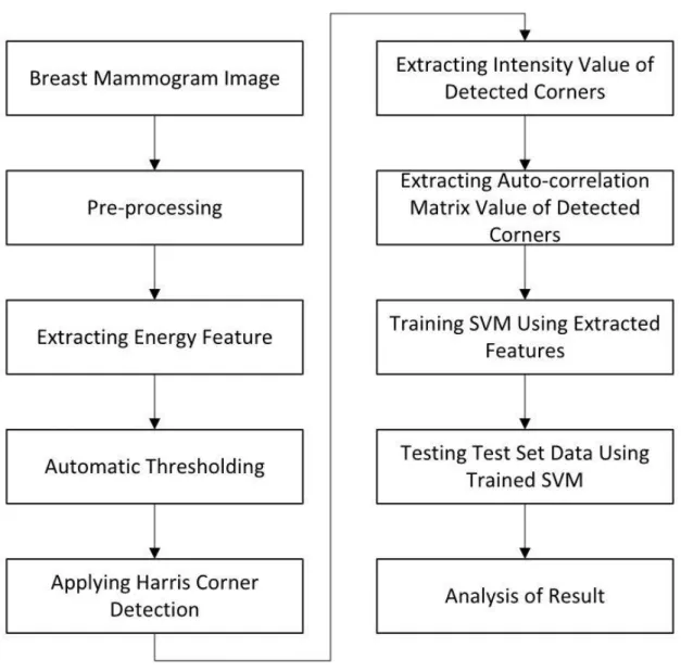
Figure 12. Flowchart of the Proposed Method ... 16
Figure 13. Sample images for both benign and malignant. a) and b) are benign, c) and d) . are malignant ... 17
Figure 14. Images, Left: gray form of original image, right: gray form of pre-processed .. image ... 19
Figure 15. Result of applying two derivatives masks on the input image. a) pre-processed input image, b) result of applying derivative mask B, c) result of applying derivative... mask A ... 21
Figure 16.Ggenerated result of corner response R... 22
Figure 18. Comparison of the proposed method in this study and two existing methods ....
(TP, FN, TN, FP). ... 27
Figure 19. Comparison of the proposed method in this study and two existing methods ....
LISTOFTABLES
Table 1. Comparison of the proposed method and two existing methods ... 25
Table 2. Comparison of the proposed method and two existing methods (%) ... 26
Table 3. Meaning of TP, FN, TN, and FP... 26
Table 4. Comparison of Precision and Recall Rate of Two Existing Methods and ...
ABSTRACT
ENHANCED BREAST CANCER CLASSIFICATION WITH AUTOMATIC
THRESHOLDING USING SUPPORT VECTOR MACHINE AND HARRIS CORNER
DETECTION
MOHAMMAD TAHERI
2017
Image classification and extracting the characteristics of a tumor are the powerful
tools in medical science. In case of breast cancer medical treatment, the breast cancer
classification methods can be used to classify input images as benign and malignant
classes for better diagnoses and earlier detection with breast tumors. However,
classification process can be challenging because of the existence of noise in the images,
and complicated structures of the image. Manual classification of the images is
time-consuming, and need to be done only by medical experts. Hence using an automated
medical image classification tool is useful and necessary. In addition, having a better
training data set directly affect the quality of classification process. In this paper, a
method is proposed based on supervised learning and automatic thresholding for both
generating better training data set, and more accurate classification of the mammogram
images into benign/malignant classes. The procedure consists of pre-processing,
removing noise, elimination of unwanted objects, features extraction, and classification.
A Support Vector Machine (SVM) is used as the supervised model in two phases which
and, energy, are three extracted features used to train the SVM. Experimental results
show this method classify images with more accuracy and less execution time compared
1. INTRODUCTION
Cancer is among the leading causes of mortality worldwide with approximately
14 million new cases and 8.2 million cancer deaths in 2012 and the number of new cases
was expected to rise by 70% over the next two decades [1]. The American Cancer
Society estimated about 231,840 new breast cancer cases for women in 2015, in 2016 it
was 249,260 new breast cancer cases and 40,890 deaths, and for 2017 the estimation is
225180 new breast cancer cases and 41,070 deaths [2][3], thus it is important to have
more studies and research about it, a summary of the estimations from 2012 to 2017 is
shown in figure 1.
Figure 1. A summary of breast cancer new cases and death estimates from 2012 to 2017
As it can be seen from figure 1 the number new cases have been increased, but the
number of death estimates has been decreased, one of the reasons is the improvements in
medical imaging and Computer Aided Diagnosis (CAD) systems. Diagnoses of
abnormality of the breast has improved using medical imaging, such as mammography,
0 50000 100000 150000 200000 250000 300000 2012 2013 2015 2016 2017
Magnetic Resonance Imaging (MRI), phantom imaging etc., thus usage of medical
images is an inevitable part of the treatment process for both early and further diagnoses.
Medical experts analyze the images to have a better understanding of the patient status
and exact location of the tumors. These medical images help doctors and medical experts
for medical treatments and analysis [4].
Detection of the abnormality in breast tissue is challenging in early detection
stage because of uncertainty in the location of the tumor. The reason is that healthy and
unhealthy part of the body have different intensity values and they are overlaid [5].
Existence of noise can also decrease the quality of the image and increase computational
time [6]. Excessive need for examination and large number of medical images to be
processed is another reason that make this process challenging [7]. Finding the correct
area of the tumor would be difficult process, even for medical experts, especially if it
must be done manually. Thus, using an efficient and reliable automated method for
classification and segmentation of the image can be led to better accuracy in detection of
the region of interest (ROI), less time spent for using the CAD system, and better
presentation of the result.
In MR imaging, some abnormalities might be selected as cancerous because it is
highly sensitive [8]. Although Mammogram images may have long execution time, they
still can be used for early detection of the tumors in breasts along with other tools such as
machine learning techniques with adequate number of input images. Machine learning
techniques can be used for classification, these techniques are based on study of patterns,
so they can make predictions based on their knowledge [9]. There are many approaches
(SVM), similarity measurement, Artificial Neural Network (ANN), genetic algorithms
and many more. An artificial neural network is a computational system for processing
information as an effort for stimulation of the real case problem, which has a set of
elements called neurons, in which they are interconnected in a multi-layer model [10].
ANN is one of the common supervised learning techniques, which can be also used for
classification, but greater computational burden, proneness to overfitting, and not having
enough training input data are some of its drawbacks [11]. In [8] ANN was used in a
smartphone based method to extract breast tumors information from Mobile Microwave
Tomography (MMT) raw data sets, but in their study they have used 30 images for both
training and testing phases which seems insufficient. SVM is another supervised learning
technique which classifies labeled data into two distinct classes [12]. In [13] SVM was
used with two input features for training phase and manual thresholding to classify
mammogram images into benign/malignant classes, using 5 different test data sets, in
which three of them were generated by themselves and the other two were used from
some existing methods, out of all of their data sets, only one data set showed better
performance. Additionally, the reported execution time is not efficient. To achieve better
result, pre-processing along with automatic thresholding are used in this study. SVM was
also used in [14] which the authors used Fuzzy Multiple-parameter SVM to tune up each
training data points by assigning suitable weight, matching to its feature, and adopts
multiple parameters as a classifier for SVM. For evaluating the method, they used total
100 mammogram images (50 benign and 50 malignant). Although their method showed
some improvements in classification of abnormalities in breast mammogram images, but
test cases. Results of this paper is compared with the proposed methods in [13] and [14]
in section 4, result and discussion. In this study SVM was used as the supervised
classifier along with automatic thresholding for better classification of the mammogram
images into two classes of malignant/benign with higher accuracy. To extract features for
training the SVM classifier, enhanced Harris Corner Detecting (HCD) along with
intensity values of the pre-processed image was used from [13], In addition energy of the
pre-processed image was added to the set of features. Energy of an image can be
calculated using the average of squared values of all of the pixels, energy can be defined
as the order of permittivity of the data [15]. Entropy was another feature used in [8] as an
input features, but it was not used it this study because as it resulted in reduction of the
accuracy of the classification. Thus, it can be said that having more input features is not
always a good idea, the goal is to increase the number of features until the accuracy of the
system reduces to it cause the system to have a long execution time. All the images went
through pre-processing for both training and testing phase, this will provide more reliable
input data sets and reduces the execution time. To improve the existing method for
classification of mammogram images into benign/malignant classes, this study focuses
for both generating better training images for the SVM classifier and better classification
of the mammogram images. In, addition, more test cases were used in this study
compared to the number of test cases used in existing methods proposed in [13] and [14].
In [13] totally 200 breast mammogram images (100 benign, 100 malignant) were used for
evaluation of the proposed method, and in [14] totally 100 breast mammogram images
(50 benign, 50 malignant) were used for evaluation of the proposed method. But in this
used for evaluation of the proposed method, in order to better evaluation of the accuracy
of the algorithm and test the performance of the proposed method under more
complicated cases.
The paper is organized as follows. Section 2 is a literature review. Section 3
describes the existing method. Section 4 explains the overall process and proposed
algorithm, which includes image acquisition, feature extraction, automatic thresholding,
and machine learning. Experimental result and comparison with existing method are
2. LITERATURE REVIEW
Feature extraction is important in terms of defining the classification systems
[16]. A feature is a function of one or more measurements, in which each of the
measurements specifies some quantifiable property of an object. Each feature quantifies
some significant characteristics of the object [17] [18].
Most image processing algorithms include some common steps as shown in
Figure 2. The first step is preprocessing of the digitized images to remove artifacts such
as patient information and reduce noise and improve quality of the image, thus features
can be extracted easier. Feature extraction is the next step which is based on finding
unique properties of an image to represent the image in terms of vector elements. All the
important information from the image is extracted in this step. After the features are
extracted, next step is to classify the images based on the extracted features. In order to
have a more accurate prediction of the medical images with less execution time, the
number of extracted features is limited [16]. In this study only three features are extracted
as with adding more features accuracy of the classification was reduced and the
computational time was increased.
Figure 2. Common steps in image processing algorithms
Features extracted from the images can be classified into two main categories:
application-independent features, such as color, texture and shape. General features
include pixel-level features, local features and global features. [18].
In this paper, the focus is on based color features as the input images are
scale mammogram images. The features are intensity value of the pre-processed
gray-scale image of the detected corner by HCD, Intensity values of the auto-correlation
3. EXISITING METHOD
3.1. Support Vector Machines (SVM)
Support vector machines are well-studied and wieldy used in machine learning as
a learning model. It is used to find patterns in the data and classify the input based on
analyzing the data [19][20][21][22].
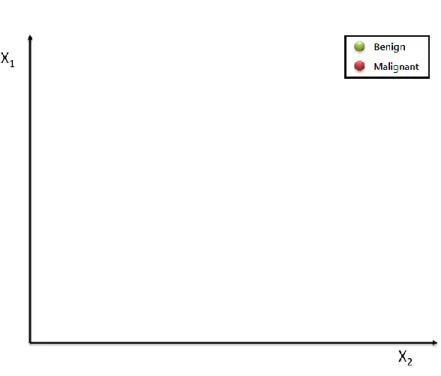
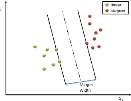
For better explanation of the SVM an example is shown in two-dimensional
feature space in figure 3. As it was mentioned in SVM there are two different phases;
testing and training. 𝑋1 and 𝑋2axis will be features as described earlier. For the training
phase, we train the algorithm by introducing the labeled data to the model.
To introduce our input data (benign and malignant images) to SVM for training
phase, we need to label the data. Thus, let’s assume that class 1 represented by red circles are malignant cases/images, and class 2 represented by green circles are benign
cases/images.
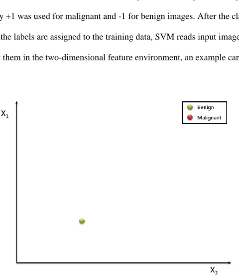
In real case, we introduce the data to the algorithm with digits or a range of digits,
for this study +1 was used for malignant and -1 for benign images. After the classes are
defined and the labels are assigned to the training data, SVM reads input images one by
one and plot them in the two-dimensional feature environment, an example can be seen in
figure 4.
Figure 4. An example of reading training images by SVM in training phase
The image in figure 4 was a benign case and shown with a green circle, SVM
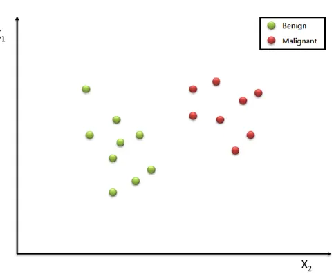
Figure 5. More training images are red by SVM in training phase
After SVM red all the input training images, the closest item of each class to the
other class is selected, figure 7.
Figure 7. Drawing lines on the closest instances of each class to the other class
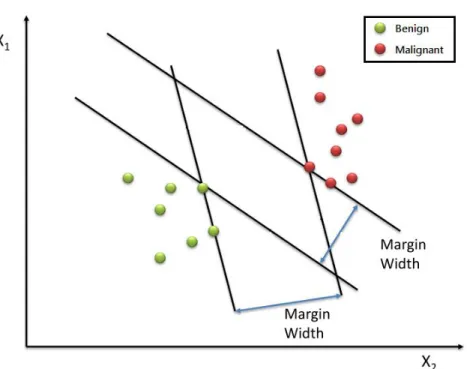
Based on the found closest items lines are drawn (black solid lines) crossing the
selected items, but as it can be seen there might be more than one way to draw the lines
on the instances of each class in which are the closest instances to the other class. The
Figure 8. Margin with maximum width
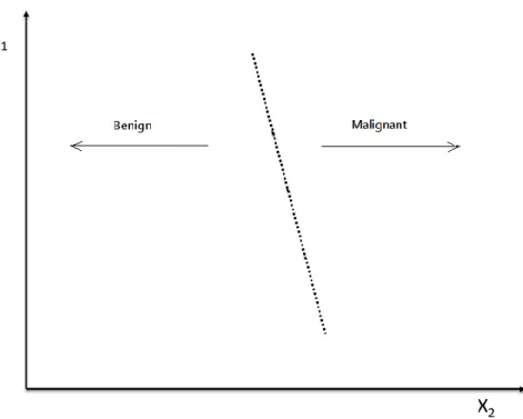
When the lines with maximum margin width are selected, a new line (dashed line)
is drawn exactly in the middle. This hyperplane is the measure of how we later classify
our unlabeled test data into the predefined classes, the final calculated hyperplane with no
Figure 9. SVM hyperplane and defined classes
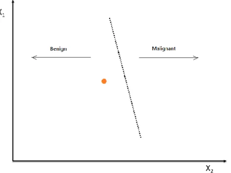
After finding the hyperplane, the training phase of the algorithm is done, now we
can use this trained model to test our test data set. But in this phase the test data is not
labeled anymore as it is the responsibility of the model to identify and classify the data.
Figure 10. An example of reading test data and classification by SVM
It can be seen the test data has no label. As the item is in the left side of the
hyperplane it would be a benign case.
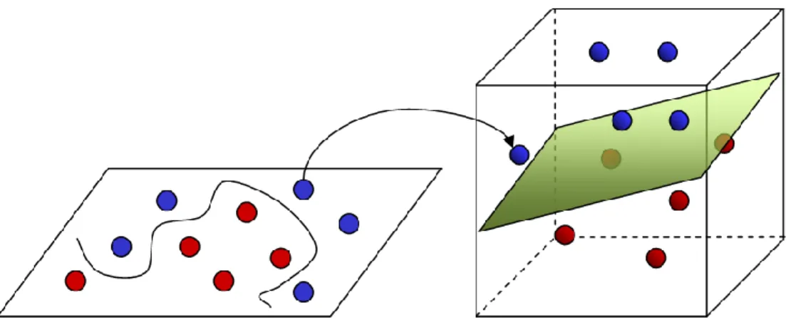
In this study, as there three features used thus, there will be a three-dimensional
feature space in which each axis represents one on the features. The feature space can be
seen in figure 11. In can be also seen that the line which separates two classes are not
4. PROPOSEDMETHOD
This study is based on combination of SVM and HCD to classify the
benign/malignant breast mammogram images [13] with using more test cases, and
automatic thresholding which increased the accuracy rate. The process is shown in figure
12.
4.1. Input Images
The input images were used in this study are gray-scale images, thus, the pixel
value is in range (0-255). Four sample input images are shown in figure 13. In which
images a) and b) are benign and c) and d) are malignant, and the tumor area is shown
inside the breast tissue. As it can be seen patient information and noise are also present in
some of the images which were removed later using pre-processing step to increase the
processing time and improving the accuracy of the algorithm.
Figure 13. Sample images for both benign and malignant. a) and b) are benign, c) and d) are malignant
4.2. Pre-Processing
This is the initial step is to be done before the main process is being started. For
the algorithm to be efficient it should deal with different images with different structures,
sizes, brightness, and resolution. Three pre-processing steps were applied to all of the
4.3. Noise Removal
The first step is to remove the noise from the images, for this purpose, there are
many filters to choose from, and here the Adaptive Median Filter (AMF) is used to
remove the noise of type salt-and-pepper [26].
Noises are removed from the mammogram images using AMF. As a nonlinear
filter, AMF with high denoising ability and efficient computational time can remove
impulse noises. In this filter, for detecting noisy pixel, the value of an output pixel will be
calculated based on the median value in a 3-by-3 neighborhood of the same pixel in the
input image [6] [27].
4.4. Removing Unwanted Objects
The second is to remove unwanted objects outside of the breast tissue in the
background. As two of the features were extracted using Harris Corner Detection (HCD)
algorithm, it is necessary to remove unnecessary extra objects to improve the
performance. In addition, if unwanted objects remain in the background, the execution
time will be increased. Execution time for removing those objects in the pre-processing
step is significantly less in comparison with the expected time of the main process, thus
Figure 14. Images, Left: gray form of original image, right: gray form of pre-processed image
4.5. Improving Image Quality
The third is to improve the quality of the mammogram image, which makes
applying the main process easier. There exist many algorithms can be used in order to
enhance the contrast of an image. Using these algorithms, more details can be extracted
and intensity contrast will be maximized [28]. For this purpose, after first two steps the
histogram of modified image is extracted and equalized [29].
4.6. Image Acquisition
600 breast mammogram images containing 300 malignant images and 300 benign
images were used. 200 out of 600 images were used for training the SVM model and the
remaining 400 images were used to testing the SVM. In some studies, such as [13]
coordinates of input images were ignored and images were used with the original
low-resolution images can improve the efficiency for pattern recognition [30][31], thus in this
study for consistency and efficiency all input images are converted to 256 by 256 pixels.
First, the images are imported to the program. These images are then sent through
pre-proceeding for noise removal and size-conversion. After pre-processing step is done,
the images were used for training the SVM, corners extracted using HCD and automatic
thresholding. Intensity value of the detected corners which has a value in range of 0 to
255 is used as one of the input training data. Values of auto-correlation matrix and energy
are other input training features.
4.7. Energy Feature
Energy of each image calculated with the equation (3) [15]:
𝐸𝑛𝑒𝑟𝑔𝑦 =1𝑛 𝛴𝑖=1𝑛 𝐼(𝑥, 𝑦)2 (3)
Where I is the processed images, x and y are coordinates of a pixel in the
pre-processed images, and n is total number of pixel in the pre-pre-processed image, as it was
mentioned earlier the size of the image will be converted to 256 by 256, thus n would be
65536.
4.8. Harris Corner Detection
A pixel is a corner region if its response is the local maximum value among all 8
surrounding neighbors [32]. So there is a significant difference between corner regions
and surrounding pixels [33].
Using HCD, some pixels in the input image were detected as corners in the
mammogram images based on values in the auto-correlation matrix. The elements of
𝑀 = [𝐴2 𝐴𝐵
𝐴𝐵 𝐵2] (4)
Where A and B are directional derivatives, defined as (5).
𝐴 = [−1 −1 −10 0 0
1 1 1
] 𝑎𝑛𝑑 𝐵 = [−1 0 1−1 0 1 −1 0 1
] (5)
Derivate masks A and B will be applied to each input image, as it can be seen in
figure 15 along with it corresponding pre-processed image.
Figure 15. Result of applying two derivatives masks on the input image. a) pre-processed input image, b) result of applying derivative mask B, c) result of applying derivative mask
A
As it can be seen some pixels inside of the breast tissue are shown as black which
means that those pixels have the value of zero. This is due to the fact that after applying
the derivative masks A and B, the result for some pixels were negative. Thus, as we know
that out input image are gray-scale image and the pixel range for this type of image as
mentioned before is in range [0-255] thus values less than zero will be mapped to zero.
Then Gaussian filter is applied to the matrix M, to generate the smoothed squared
𝑅 = 𝐷𝑒𝑡𝑒𝑟𝑚𝑖𝑛𝑎𝑛𝑡(𝑀) − (0.04 ∗ 𝑇𝑟𝑎𝑐𝑒2(𝑀)) (6)
An example of generated result of corner response R can be seen in figure 16, this image
is a gray-scale image, but for better visualization is converted to a black and white image.
Figure 16.Ggenerated result of corner response R
A pixel will be detected as corner if the value of its response is greater than a
specific threshold. This threshold can be set either manually or automatically [32]. In [13]
manual thresholding was used to find the optimum threshold. In this study, automatic
thresholding was used. The result can be seen in figure 17, a) is the original image with
the tumor area shown, b) the detected corners, and c) detected corners on the
Figure 17. Result of corner response R after applying the automated thresholding
These detected corner pixels can be used as training feature of SVM along with
other features for the purpose of classification [13]. Based on the investigating of the
sample test cases, malignant cases have more detected corners than benign cases.
4.9. Support Vector Machine
SVM is a supervised learning model for classification of data implemented based
on a separating hyperplane. There are two major steps: training and testing. First the
algorithm is trained using labeled data for different classes. To classify data, the
algorithm generates a hyperplane which separates different classes and assign every input
of test set data to one of the defined classes [9][12].
4.10. Automatic Thresholding
Thresholding can be selected using both manual thresholding and automatic
thresholding. If the threshold is selected manually, it might be optimum for a specific
image or set of images, but not for different type of images. Using automatic
this study, automatic thresholding was used and based on the result it can be said that the
method is more accurate compared to methods using manual thresholding.
There are different automatic thresholding algorithms, and the one used for this
study was for computing an optimal threshold for separating the data into two classes,
and can be summarized as follows. First the histogram of the input mammogram image is
computed, and a random threshold value is set. Using the starting randomly selected
threshold the histogram is divided into two parts. Thus, data can be classified into two
distinct classes, now the mean of each class is calculated, and a new threshold was
calculated as the average of two classes’ means. This process will be continued until there is no new value for threshold [34] [35].
4.11. Classification
To train the SVM algorithm two classes were defined as malignant and benign,
where each class has a unique label; +1 for malignant and -1 for benign images, along
with extracted features. Using the trained SVM classifier, for each input image, the
output is an array of labels, called as prediction array. After the SVM is trained using
those three features, it was tested using 400 mammogram images, 200 malignant and 200
5. EXPERIMENTALRESULTSANDANALYSIS
To have a better evaluation of the proposed method in addition to previous steps
discussed earlier, the number of test cases was also increased to test the proposed method
under more complicated cases. Thus, in this paper the number of test cases was increased
up to 400 (200 benign and 200 malignant), compared to existing method 1 [13] and
method 2 [14] respectively 200, and 100. In this study, totally 600 mammogram images
were used, the images were used is the subset of the same database used in [13] . Based
on the method discussed in section 3.1 an image was classified as benign if the total
number of plus ones are greater than total number minus ones and vice versa, this method
is called ResultByCount [13]. Table 1 and 2 show correctly classified and misclassified
images, the only difference between table 1 and 2 is that the numbers in table 2 are
percent, and meaning of the labels in table 1 and table 2 are described in table 3.
To have a better evaluation of the results, the experimental result is also compared
with proposed result in existing method 1 in [13] and existing method 2 in [14], in table
1, table 2, table 4 and figure 18 and figure 19.
Table 1. Comparison of the proposed method and two existing methods
Existing Method 1 (out of 100) Existing Method 2 (out of 50) Proposed Method (out of 200) TP 91 48 185 FN 9 2 15 TN 92 45 194 FP 8 5 6
Table 2. Comparison of the proposed method and two existing methods (%)
Existing Method 1 Existing Method 2 Proposed Method
TP (%) 91 96 92.5
FN (%) 9 4 7.5
TN (%) 92 90 97
FP (%) 8 10 3
Table 3. Meaning of TP, FN, TN, and FP
Labels Meaning
True Positive (TP) malignant detected as malignant
False Negative (FN) malignant detected as benign
True Negative (TN) benign detected as benign
False Positive (FP) benign detected as malignant
Precision and sensitivity (recall rate) can also be calculated in order to measure
the accuracy of the proposed classification algorithm with the equations (7) and (8).
𝑃𝑟𝑒𝑐𝑖𝑠𝑖𝑜𝑛 =𝑇𝑃+𝐹𝑃𝑇𝑃 ∗ 100 (7) 𝑆𝑒𝑛𝑠𝑖𝑡𝑖𝑣𝑖𝑡𝑦 =𝑇𝑃+𝐹𝑁𝑇𝑃 ∗ 100 (8)
Table 4. Comparison of Precision and Recall Rate of Two Existing Methods and Proposed Method.
Existing Method 1 Existing Method 2 Proposed Method Precision (%) 92 90.6 96.8 Sensitivity (%) 91 96 92.5
Precision can be referred as Positive Predicted Value (PPV), and recall rate as
positive rate or sensitivity [36]. Figure 18 and figure 19 show the comparison between
the proposed method in this study and existing method 1 used in [13] and existing
method 2 used in [14] which the authors used Fuzzy Multiple-parameter SVM.
Figure 18. Comparison of the proposed method in this study and two existing methods (TP, FN, TN, FP).
Figure 19. Comparison of the proposed method in this study and two existing methods (Precision and Sensitivity).
According to the figure 18, and figure 19, the proposed method in this paper
showed better performance than both existing method 1 and 2, and better performance
than existing method 1 in term of sensitivity. Existing method 2 showed better
performance in term of classification of true positive and sensitivity, but as it was
mentioned in result and discussion they used only 100 test cases to evaluate their method
6. CONCLUSIONS
SVM is a popular classification method and has been used in different areas, such
as medical image classification. Thus, it can be used for better early detection of
abnormalities in a breast tissue. Using suitable and the right number of training features,
along with right number of training inputs, we can improve the accuracy, and efficiency
of the SVM model for classification, and reduce the execution time. In addition, better
results are generated as an effect of using pre-processing, and automatic thresholding,
pre-processing step was used for both training and testing the algorithm. This study
classified benign/malignant mammogram images using combination of SVM and
automatic thresholding based-Harris Corner Detection. The results show that the
proposed method has a better accuracy in classification of benign/malignant mammogram
images when compared to previous research studies. The experimental result implies that
using proposed method, more reliable result can be generated for early and further
REFERENCES
[1] “Organization, W.H., 2014. World Cancer Report, 2014. WHO Report. Geneva: WHO.”
[2] “Cancer Facts & Figures 2015. American Cancer Society.,” 2015. [3] “Cancer Statistics Center.” [Online]. Available:
https://cancerstatisticscenter.cancer.org/?_ga=1.242628866.1838802877.14640450
43#/.
[4] B. C. C, K. Rajamani, and L. V L, “A Review on Automatic Marker Identification Methods in Watershed Algorithms Used for Medical Image Segmentation,” IJISET -International J. Innov. Sci. Eng. Technol., vol. 2, no. 9, 2015.
[5] N. Kumar and S. Arora, “Medical Evaluation of Marker Controlled Watershed Technique for Detecting Brain Tumors,” Int. J. Comput. Appl., vol. 54, no. 11, pp. 975–8887, 2012.
[6] R. H. Chan, C.-W. Chung-Wa, and M. Nikolova, “Salt-and-pepper noise removal
by median-type noise detectors and detail-preserving regularization,” IEEE Trans.
Image Process., vol. 14, no. 10, pp. 1479–1485, Oct. 2005.
[7] P. Jagya, “Comparison of Two Segmentation Methods for Mammographic Image,” vol. 126, no. 1, pp. 31–43, 2015.
[8] S. Aminikhanghahi, W. Wang, S. Shin, S. H. Son, and S. I. Jeon, “Effective tumor
feature extraction for smart phone based microwave tomography breast cancer
Computing - SAC ’14, 2014, pp. 674–679.
[9] E. Alpaydin, Introduction to Machine Learning, Second Edi. MIT Press, 2004.
[10] ARTIFICIAL INTELLIGENCE : concepts, methodologies, tools, and applications. INFORMATION SCI REFER IGI, 2017.
[11] J. Liu, J. Chen, X. Liu, L. Chun, J. Tang, and Y. Deng, “Mass segmentation using
a combined method for cancer detection.,” BMC Syst. Biol., vol. 5 Suppl 3, no. Suppl 3, p. S6, 2011.
[12] N. C. and J. Shawe-Taylor, An Introduction to Support Vector Machines: And
Other Kernel-Based Learning Methods. New York, NY, USA: Cambridge
University Press, 1999.
[13] H. I. Kim, S. Shin, W. Wang, and S. I. Jeon, “SVM-based Harris Corner Detection
for Breast Mammogram Image Normal / Abnormal Classification,” pp. 187–191. [14] C. Pack, S. Shin, S. H. Son, and S. I. Jeon, “Computer Aided breast cancer
Diagnosis system with Fuzzy Multipleparameter Support Vector Machine C3 -
Proceeding of the 2015 Research in Adaptive and Convergent Systems, RACS
2015,” Res. Adapt. Converg. Syst. RACS 2015, pp. 172–176, 2015.
[15] M. Wadhwani, S., Wadhwani, A.K. and Saraswat, “Classification of Breast Cancer
Detection Using Artificial Neural Networks,” Eng. Sci. Technol., vol. 1, no. 3, pp. 85–91, 2013.
[16] M. F. Akay, “Support vector machines combined with feature selection for breast
[17] R. S. Choras, “Image feature extraction techniques and their applications for CBIR
and biometrics systems,” Int. J. Biol. Biomed. Eng., vol. 1, no. 1, pp. 6–16, 2007. [18] R. Kasaudhan, T. K. Heo, S. I. Jeon, and S. H. Son, “Similarity measurement with
mesh distance fourier transform in 2D binary image,” in Proceedings of the 2015 Conference on research in adaptive and convergent systems - RACS, 2015, pp.
183–187.
[19] E. Osuna, R. Freund, and F. Girosi, “Training Support Vector Machines: an
Application to Face Detection,” Proc. 1997 Conf. Comput. Vis. Pattern Recognit. (CVPR ’97), pp. 130–37, 1997.
[20] M. Pontil and A. Verri, “Support Vector Machines for 3D Object Recognition,”
Patern Anal. Mach. Intell., vol. 20, no. 6, pp. 637–646, 1998.
[21] A. G. L. Neves, R.P., Zanchettin, C., and Filho, “An Efficient Way of Combining
SVMs for Handwritten Digit Recognition,” Artif. Neural Networks Mach. Learn., pp. 229–237.
[22] O. Chapelle, P. Haffner, and V. N. Vapnik, “Support vector machines for
histogram-based image classification,” IEEE Trans. Neural Networks, vol. 10, no.
5, pp. 1055–1064, 1999.
[23] J. Moon, H. I. Kim, H. D. Choi, and S. I. Jeon, “A Support Vector Machine based
Classifier to Extract Abnormal Features from Breast Magnetic Resonance
Images.”
DNA sequences,” TOP, vol. 18, no. 2, pp. 339–353, Dec. 2010.
[25] P. Gaspar, J. Carbonell, and J. L. Oliveira, “On the parameter optimization of
Support Vector Machines for binary classification.,” J. Integr. Bioinform., vol. 9, no. 3, p. 201, Jul. 2012.
[26] C. Ning, S. Liu, and M. Qu, “Research on removing noise in medical image based
on median filter method,” in 2009 IEEE International Symposium on IT in Medicine & Education, 2009, vol. 1, pp. 384–388.
[27] H. Hwang and R. A. Haddad, “Adaptive median filters: new algorithms and
results,” IEEE Trans. Image Process., vol. 4, no. 4, pp. 499–502, Apr. 1995. [28] I. K. Maitra, S. Nag, and S. K. Bandyopadhyay, “Technique for preprocessing of
digital mammogram,” Comput. Methods Programs Biomed., vol. 107, no. 2, pp. 175–188, 2012.
[29] Gonzalez and Woods, Digital Image Processing, 3rd edition. Prentice Hall.
[30] and A. N. A.-R. Khuwaja, Gulzar A., “Bi-modal breast cancer classification
system,” Pattern Anal. Appl., vol. 7, no. 3, p. 235–242., 2004.
[31] G. A. Khuwaja, “An Adaptive Combined Classifier System for Invariant Face
Recognition,” Digit. Signal Process., vol. 12, no. 1, pp. 21–46, Jan. 2002.
[32] C. Harris and M. Stephens, “A Combined Corner and Edge Detector,” Procedings
Alvey Vis. Conf. 1988, p. 23.1-23.6, 1988.
[33] C. Harris, Geometry from visual motion. Cambridge, MA, USA: MIT Press, 1993.
Iterative Selection Method,” no. 8, 1978.
[35] D. Ramachandram, “Automatic Thresholding.” [Online]. Available:
http://www.mathworks.com/matlabcentral/fileexchange/loadFile.do?objectId=319
5&objectType=file.