Parallel one-versus-rest SVM training on the GPU
Sander Dieleman*, A¨aron van den Oord*, Benjamin Schrauwen Electronics and Information Systems (ELIS)
Ghent University, Ghent, Belgium
{sander.dieleman, aaron.vandenoord, benjamin.schrauwen}@ugent.be
* Both authors contributed equally to this work.
Abstract
Linear SVMs are a popular choice of binary classifier. It is often necessary to train many different classifiers on a multiclass dataset in a one-versus-rest fashion, and this for several values of the regularization constant. We propose to harness GPU parallelism by training as many classifiers as possible at the same time. We optimize the primal L2-loss SVM objective using the conjugate gradient method, with an adapted backtracking line search strategy. We compared our approach to liblinear and achieved speedups of up to 17 times on our available hardware.
1
Introduction
In recent years, linear SVMs have been a popular choice to evaluate the discriminative performance of features extracted with novel unsupervised feature learning methods [3, 5, 8, 9]. In this setting, it is required to train many different classifiers on the same dataset, but with different labelings: when using a one-versus-rest approach, a separate classifier must be trained for each class. Furthermore, several possible values for the regularization constant have to be evaluated.
In this paper, we propose to speed up this process by training as many classifiers as possible at the same time, instead of parallelizing the training procedure of a single classifier. If there arenclasses, andmdifferent values of the regularization constant are tried, the total number of classifiers that are trained on the same dataset isn·m. This value is typically high enough for GPU parallelism to be beneficial. Since GPUs are becoming more and more prevalent in research environments, our approach provides a worthwhile alternative to using a computer cluster to speed up classifier training.
2
Approach
We start with the primal formulation of the L2-loss SVM optimization problem for a single classifier [4]. Note that the following approach can also be used for most other typical loss functions, such as the L1 or logistic loss. LetXbe a design matrix withlexamplesxi, and letybe a vector containing the corresponding labelsyi. Letwbe the parameters of the model andCbe a regularization constant. The objective is then1:
min1 2||w|| 2+C l X i=1 1−yiwTxi 2 +. (1)
Consider the setting wherenclassifiers are trained, using the same dataX, but with a different set of labelsyk, and a different regularization constantCk. Each classifier also has its own parameter
1
vectorwkand its own objective functionJk(wk). We can group the parameter vectors into a matrix W withncolumns, and the labels can similarly be grouped into a matrixY. We then propose to compute the following weighted sum of the objective functions:
J(W) = n X k=1 Jk(wk) Ck = n X k=1 ||wk||2 2Ck +1 T 1−Y ◦WTX2 +1, (2)
where◦represents an elementwise product of two matrices,1represents a vector with all elements equal to1, and1represents a matrix with all elements equal to1. By weighting the terms with the inverse of their corresponding regularization constants, we ensure that their gradients will be of a comparable order of magnitude.
If we optimize thejoint objective functionJ(W), we are also optimizing the individual terms of the sum, i.e. theconstituent objective functionsJk(wk), because they share no parameters.J(W)
contains the subexpressionWTX, which is a matrix-matrix product. This makes it more amenable to GPU acceleration, which is the basis of our approach. Note that this function is convex, because it is a sum of convex functions.
3
Parallel conjugate gradient
We used the conjugate gradient (CG) method [6] to minimize the joint objective functionJ(W), in combination with a backtracking line search, as described by Boyd and Vandenberghe [2]. The CG algorithm is oblivious to the compositional nature of the objective function, except for the line search component.
CG relies on a line search to determine the step size during every iteration. A naive approach would be to use an unadapted line search strategy, which ignores the fact thatJ(W)is the sum of several independent objective functions. However, this would be very inefficient, because it would only enforce a decrease inJ(W), but not necessarily in the constituent objective functions. It might select a step size that decreases the value of some of them, while increasing the value of others to a lesser extent.
One could perform a separate line search for each constituent objective function. However, in light of our goal of harnessing GPU parallelism, this is problematic: the line search requires the evaluation of the objective functions at different candidate step sizes, and we can only take advantage of GPU parallelism if we evaluate allJk(wk)at once. Each line search would require a different number of evaluations, so we would have to evaluate all constituent objective functions as many times as the maximal number of required evaluations across all of them. This would lead to a lot of unnecessary computation.
Instead, we propose to perform only as many evaluations as are necessary to sufficiently reduce the joint objective function J(W), and then to select the optimal step size separately for each of the parameter vectorswk, based on the values of the constituent objective functionsJk(wk). Recall thatJ(W)is a weighted sum of allJk(wk), so we have already computed their values for different step sizes at this point. Although this does not guarantee that all of them will decrease, it does ensure that they will never increase (i.e. a step size of zero might be selected for some).
We used the same convergence criterion asliblinear’s primal L2-loss SVM solver [4]. All parameter values are initialized to zero. The optimization is stopped when the norm of the gradient is smaller than a fraction of the norm of the initial gradient:
||∇Jk(wk)||< ε·min(l p k, l n k) l · ||∇Jk(0)||. (3)
Here,εis a chosen tolerance constant,lis the number of data points, andlpk,ln
k are the number of datapoints with positive and negative labels respectively. This means that the convergence criterion depends on the imbalance of the dataset (more imbalance leads to a smaller fraction).
Because not all classifiers will converge at the same time, we modify the objective functionJ(W)
during the optimization by removing converged classifiers from it. Since we can only evaluate all Jk(wk)at once, this avoids a lot of unnecessary computation.
CPU GPU
model frequency # cores model # cores RAM
A Core i7 930 2.80 GHz 4 GeForce GTX 480 480 1.5 GB
B Core i7 860 2.80 GHz 4 GeForce GTX 560 Ti 384 1 GB
C Xeon E5504 2.00 GHz 4 Tesla C1060 240 4 GB
D Core i7 2670QM 2.20 GHz 4 GeForce GT 540M 96 2 GB
E Core 2 Q9550 2.83 GHz 4 n/a n/a n/a
Table 1: Specifications of the different machines that were used to run the experiments. All of them have Intel CPUs and NVIDIA GPUs.
10-1 100 101 102 103 total training duration [minutes]
50 55 60 65 70 75 80
max accuracy [percent] proposed (A)proposed (B)proposed (C) proposed (D) liblinear (E) liblinear (B)
(a) CIFAR-10 (100 classifiers)
100 101 102 103 total training duration [minutes] 25 30 35 40 45 50
max accuracy [percent] proposed (A)
proposed (C) proposed (D) liblinear (E)
(b) CIFAR-100 (500 classifiers)
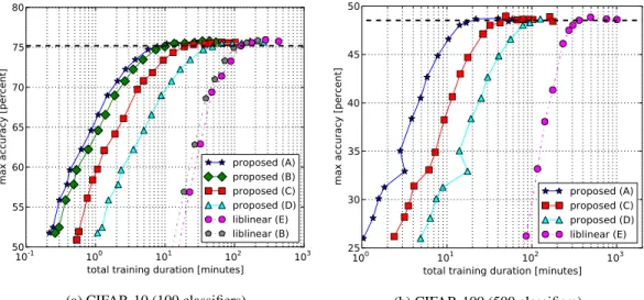
Figure 1: Total training duration for different values of the tolerance constantε, versus the best achievable classification accuracy over all values ofC at each point. The letters indicate the ma-chines the experiments were run on (see Table 1). The horizontal dashed lines indicate the reference accuracy levels used to determine the speedups in Table 2.
4
Implementation
We used theTheanopackage for Python [1]. Theano allows for mathematical expressions to be formulated symbolically, and is capable of compiling these into efficient code for execution on CPUs or GPUs with CUDA support. Furthermore, it supports automatic differentiation. This made it possible to implement our approach quickly and easily, by formulating expression 2 in Theano, and having it compute the necessary gradients, as well as compile the resulting code to enable GPU acceleration. To avoid costly transfers between CPU and GPU memory, the data and labels are stored on the GPU at the start of the algorithm.
The backtracking line search algorithm has a couple of hyperparameters [2]. Since the objective function is convex, these hyperparameters do not affect the end result, but they do affect the speed of convergence. We fixed them to values that result in an acceptable rate of convergence across a number of different datasets.
5
Experiments and results
To assess the merit of our approach, we compared it to the de facto standard for training linear SVM classifiers:liblinear[4]. In a first experiment, we trained classifiers on features extracted from the CIFAR-10 dataset [7], using the soft K-means approach of Coates et al. [3]. We used the code they made available to extract 800 features from the dataset.
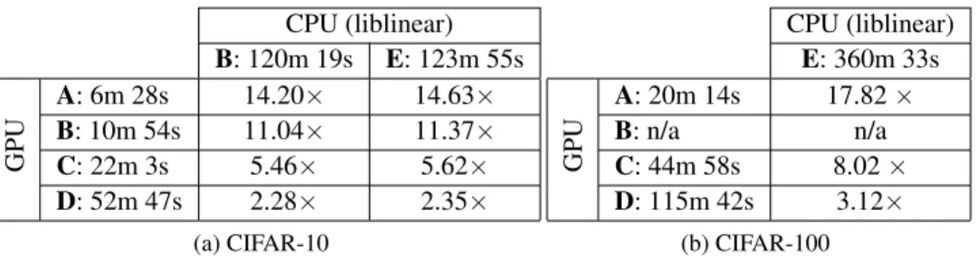
CPU (liblinear) B: 120m 19s E: 123m 55s GPU A: 6m 28s 14.20× 14.63× B: 10m 54s 11.04× 11.37× C: 22m 3s 5.46× 5.62× D: 52m 47s 2.28× 2.35× (a) CIFAR-10 CPU (liblinear) E: 360m 33s GPU A: 20m 14s 17.82× B: n/a n/a C: 44m 58s 8.02× D: 115m 42s 3.12× (b) CIFAR-100
Table 2: Speedup of our approach over liblinear when comparing different GPUs and CPUs, at the reference accuracy levels indicated on Figure 1.
On this dataset, which consists of natural images of objects divided into 10 classes (50,000 for training, 10,000 for testing), we trained a set of one-versus-rest classifiers. We did this for 10 different values of the regularization constantC, spaced evenly on a log scale between 10−5and
105. This amounts to 100 classifiers in total being trained on the same dataset. We repeated this experiment for different values of the constantε, which is used to determine convergence.
First, we trained the classifiers sequentially using liblinear, which was compiled with the Intel Math Kernel Library to ensure a fair comparison. Then, we trained them in parallel using our approach on several different GPUs. The specifications of the machines we used for these experiments are listed in Table 1. Figure 1a shows the total training duration for 100 classifiers for different values ofε, versus the best achievable classification accuracy on the test set over all values ofCat each point. Next, we performed the same experiment on the CIFAR-100 dataset. This dataset is similar to CIFAR-10 and has the same size, but it has 100 different object classes. We used only 5 different values ofCthis time, spaced evenly on a log scale between10−3and103, resulting in 500 classifiers to be trained in total. We were unable to run this experiment on machine B, because it has only 1 GB of GPU memory and this turned out to be insufficient. The results of this experiment are shown in Figure 1b.
The relative speedups of our approach over liblinear for both datasets at reference accuracy levels (indicated in Figure 1) are listed in Table 2. The reference accuracy levels were chosen using the default stopping criterium of liblinear on machine E. The speedups seem to depend strongly on the number of CUDA cores of the GPU.
6
Conclusion and future work
Our approach shows promising results: significant speedups are achieved over liblinear, the current standard in linear SVM training. We were able to achieve speedups of up to 17×on our available hardware. This makes it a valuable alternative to using liblinear on a computer cluster. The most recent generation of GPUs have a much larger number of cores than the ones we tested; as this trend continues, the advantage of our approach will only increase.
We would like to extend this work in two main directions: developing our research code into a usable tool, and making the approach more broadly applicable. Currently, it is restricted to situations where the entire dataset can fit in GPU memory, and the maximal number of classifiers that can be trained in parallel is memory-limited as well. We would like to investigate how we can deal with larger datasets that are read into GPU memory in batches, while avoiding any delays due to memory transfers. This may require extensions to Theano.
Furthermore, we would like to be able to train classifiers on subsets of a given dataset. This would enable the parallelization of one-versus-one classifier training, and even cross-validation. We would also like to look into stochastic methods for SVM classifier training, and extend our approach to kernel SVMs.
References
[1] James Bergstra, Olivier Breuleux, Fr´ed´eric Bastien, Pascal Lamblin, Razvan Pascanu, Guillaume Des-jardins, Joseph Turian, David Warde-Farley, and Yoshua Bengio. Theano: a CPU and GPU math expression compiler. InProceedings of the Python for Scientific Computing Conference (SciPy), June 2010.
[2] Stephen Boyd and Lieven Vandenberghe. Convex Optimization. Cambridge University Press, New York, NY, USA, 2004. ISBN 0521833787.
[3] Adam Coates, Andrew Y. Ng, and Honglak Lee. An analysis of single-layer networks in unsupervised feature learning.Journal of Machine Learning Research - Proceedings Track, 15:215–223, 2011. [4] Rong-En Fan, Kai-Wei Chang, Cho-Jui Hsieh, Xiang-Rui Wang, and Chih-Jen Lin. LIBLINEAR: A library
for large linear classification.Journal of Machine Learning Research, 9:1871–1874, 2008.
[5] Mikael Henaff, Kevin Jarrett, Koray Kavukcuoglu, and Yann LeCun. Unsupervised learning of sparse features for scalable audio classification. In Anssi Klapuri and Colby Leider, editors,ISMIR, pages 681– 686. University of Miami, 2011. ISBN 978-0-615-54865-4.
[6] Magnus R. Hestenes and Eduard Stiefel. Methods of Conjugate Gradients for Solving Linear Systems. Journal of Research of the National Bureau of Standards, 49(6):409–436, December 1952.
[7] Alex Krizhevsky. Learning Multiple Layers of Features from Tiny Images. Master’s thesis, 2009. [8] Honglak Lee, Peter Pham, Yan Largman, and Andrew Ng. Unsupervised feature learning for audio
clas-sification using convolutional deep belief networks. In Y. Bengio, D. Schuurmans, J. Lafferty, C. K. I. Williams, and A. Culotta, editors,Advances in Neural Information Processing Systems 22, pages 1096– 1104. 2009.
[9] J. W¨ulfing and M. Riedmiller. Unsupervised learning of local features for music classification. In Proceed-ings of the 13th International Society for Music Information Retrieval Conference (ISMIR), 2012.