University of Windsor University of Windsor
Scholarship at UWindsor
Scholarship at UWindsor
Major Papers Theses, Dissertations, and Major Papers June 2020
On Variable Selections in High-dimensional Incomplete Data
On Variable Selections in High-dimensional Incomplete Data
TAO SUNDepartment of Mathematics and Statisticshigh-dimensional data; missing value; variable selection; missForest; self-training selection; random lasso; stability selection; Meta-analysis, [email protected]
Follow this and additional works at: https://scholar.uwindsor.ca/major-papers
Part of the Applied Statistics Commons, and the Biostatistics Commons
Recommended Citation Recommended Citation
SUN, TAO, "On Variable Selections in High-dimensional Incomplete Data" (2020). Major Papers. 128.
https://scholar.uwindsor.ca/major-papers/128
This Major Research Paper is brought to you for free and open access by the Theses, Dissertations, and Major Papers at Scholarship at UWindsor. It has been accepted for inclusion in Major Papers by an authorized administrator of Scholarship at UWindsor. For more information, please contact [email protected].
In High-dimensional Incomplete Data
by
TAO SUN
A Major Research Paper
Submitted to the Faculty of Graduate Studies
through the Department of Mathematics and Statistics
in Partial Fulfillment of the Requirements for
the Degree of Master of Science at the
University of Windsor
Windsor, Ontario, Canada
c
On Variable Selections
In High-dimensional Incomplete Data
by
TAO SUN
APPROVED BY:
—————————————————————–
A. Hussein
Department of Mathematics and Statistics
—————————————————————–
S. Nkurunziza, Advisor
Department of Mathematics and Statistics
I hereby certify that I am the sole author of this major paper and that no part of
this major paper has been published or submitted for publication.
I certify that, to the best of my knowledge, my major paper does not infringe upon
anyone’s copyright nor violate any proprietary rights and that any ideas, techniques,
quotations, or any other material from the work of other people included in my major
paper, published or otherwise, are fully acknowledged by the standard referencing
practices. Furthermore, to the extent that I have included copyrighted material that
surpasses the bounds of fair dealing within the meaning of the Canada Copyright
Act, I certify that I have obtained written permission from the copyright owner(s) to
include such material(s) in my major paper and have included copies of such copyright
clearances to my appendix.
I declare that this is a true copy of my major paper, including any final revisions,
as approved by my major paper committee and the Graduate Studies office, and that
this major paper has not been submitted for a higher degree to any other University
or Institution.
Abstract
Modern Statistics has entered the era of Big Data, wherein data sets are too large,
high-dimensional, incomplete and complex for most classical statistical methods. This
analysis of Big data firstly focuses on missing data. We compare different multiple
im-putation methods. Combining the characteristics of medical high-throughput
exper-iments, we compared multivariate imputation by chained equations (MICE), missing
forest (missForest), as well as self-training selection (STS) methods. A phenotypic
data set of common lung disease was assessed. Moreover, in terms of improving the
interpretability and predictability of the model, variable selection plays a pivotal role
in the following analysis. Taking the Lasso-Poisson model as an example, we
illus-trate the robust random Lasso method in the Meta-analysis of multiple datasets for
variable selection. Thus, the real data analysis clarifies that missForest and STS
outperform MICE. Moreover, the simulation results show that although this method
is as effective in selecting important variables as using the random Lasso method,
meta-analysis based on the random Lasso is better in terms of coefficient estimation
and elimination of unimportant variables. In conclusion, We firstly propose a
miss-Forest random lasso (MFRL) method to complete the multiple imputation of the
high-dimensional data and robustly select important variables.
Key Words: high-dimensional data; missing value; variable selection; missForest; self-training selection; random lasso; stability selection; Meta-analysis
vi
To my loving Family
This major paper could not have been possible without the help and the support of
several individuals. First and foremost, I would like to express my deepest gratitude
to my beloved supervisor, Dr. S´ev´erien Nkurunziza, for his immense support and
extremely valuable guidance throughout my statistical master study. Without his
consistent and illuminating instruction, I would not be where I am today. I not only
learned new statistical knowledge from him but also learned how to conduct research
with creativeness and better vision. His enthusiasm to help his students will always
be a good example and guide me in my future.
I would also like to thank Dr. Abdul A. Hussein for being my department reader.
He also taught me the basic knowledge of Time Series and Survival Analysis, which
helped me build a solid foundation for further studies in Statistics.
In addition, I would like to thank all faculty and staff members, and the graduate
students in the Department of Mathematics and Statistics who helped me in many
different ways during my study.
It is the dream of everyone to play an important role on the stage surrounded
by loyal audiences. However, our sense of security, hopefulness, confidence, and
self-worth are built by members of our family who can hold our hands tightly even in
viii
the midst of I think myself a lucky fellow to have such supportive family members.
Especially, my wife, Yuejing Yang, and my daughters whose unwavering support and
Author’s Declaration of Originality iii Abstract v Dedication vi Acknowledgments viii List of Tables xi 1 Introduction 1 1.1 Missing Data . . . 2
1.2 Variable Selection in High-dimensional Data . . . 6
2 Literature Review 9 2.1 Progress in Research . . . 10
2.2 Trends in Research Development . . . 13
2.3 Existing Work on Multiple Imputation . . . 15
2.3.1 Multiple Imputation Algorithm . . . 15
2.3.2 missForest . . . 19
CONTENTS x
2.3.3 The Self-training Selection (STS) Scheme . . . 22
2.4 Assessment of Imputation Performance . . . 24
2.4.1 Evaluating the Methods . . . 24
2.5 A Variable Selection Method - Random Lasso . . . 25
2.5.1 Limitations and Improvements of Lasso . . . 25
2.5.2 The Principle of Random Lasso . . . 28
2.5.3 The Algorithm of Random Lasso . . . 29
3 Numerical Results 32 3.1 Analysis in Real Data (COPD Dataset) . . . 32
3.2 Simulation Results . . . 37
4 Concluding Remarks 44
Bibliography 46
3.1 Coefficient estimate of the important explanatory variables . . . 40
3.2 Coefficient estimate of the unimportant explanatory variables . . . . 41
3.3 Average RME times 100 . . . 41
3.4 Numbers of unimportant variables to be selected . . . 42
Chapter 1
Introduction
Recently, the research of variable selections in high-dimensional incomplete data has
attracted a lot of attention. This kind of study includes two parts, missing data and
variable selections.
Missing data are commonly encountered in many data analyses. High-dimensional
data sets often lead to biased or less precise results under traditional statistical
meth-ods. Importantly, this problem has begun to be solved by the data mining methods,
aided by the rapidly developing computational power of artificial intelligence (Lee
and Siau (2001) [30]).
In addition, high-dimensional data present new challenges for variable selection in
regression analysis. Variable selection plays a pivotal role in regression analysis as it
identifies important variables that are associated with outcomes and have been shown
to improve predictive accuracy and interpretability of the resulting models. Variable
selection methods have been widely investigated for complete data including
classi-cal model selection methods, penalization methods and Bayesian variable selection
methods (Fan and Lv (2010) [15]).
1.1
Missing Data
In medicine, finance, transportation, telecommunications and a variety of other fields,
missing data are commonly encountered (Lee and Siau (2001) [30]). Since all
statis-tical analysis techniques strictly derive information from data sets, the quality of the
information depends to a large extent on the deviation of the data set. As one of the
important factors affecting the behavior of data, missing data may not only cause the
deviation of the estimator but also lead to the distortion of the estimator variance,
which reduces the efficiency of traditional statistical methods (Kang (2013) [26]).
Therefore, statistical approaches coping with missing data have naturally become a
crucial issue for researchers.
To introduce some notations, let X be a fully observable d-dimensional covariate.
Further, let Xobs be the observed value, let Xmis be the missing value and let δ be
the missing indicator function.
In term of missing data and data dependencies, Little and Rubin ((1989) [34])
clas-sify the missing data mechanisms into three categories: (1) Missing not at random
vari-CHAPTER 1. INTRODUCTION 3
able. That is, P(δ = 1|Xobs, Xmis) 6= P(δ = 1|Xobs). When δ = 0, it means the
data is observable. When δ = 1, it means the data is missing. (2) Missing at
random (MAR) (Rosenbaum and Rubin (1983) [49]): the missingness is not
ran-dom, but the probability of missing data depends on the value of the observable
variable in the sample. MAR provides asymptotically unbiased estimates. That
is, P(δ = 1|Xobs, Xmis) = P(δ = 1|Xobs) = π(Xobs), where π(z) is the selection
probability function. (3) Missing completely at random (MCAR): Whether the
data is missing or not does not depend on any observed or missing data. That
is, P(δ = 1|Xobs, Xmis) = P(δ = 1). MAR is the most commonly used in statistical
research (Little and Rubin (1989) [34]). Therefore, the missing mechanism of this
paper is based on this MAR assumption.
Historically, the approaches for dealing with missing data in the past can be classified
into three categories: deleting cases with missing values, grouping cases with
miss-ing values as a new class of values and fillmiss-ing cases with missmiss-ing values. Firstly, the
simplest method of dealing with missing data is the complete data analysis method,
which consists of deleting the missing data and solely using the fully observed data for
statistical inference. Because the missing data information is ignored, this method
will lead to the loss of statistical efficiency. Meanwhile, if the missing data is not
completely at random, the estimates obtained by this method are usually biased.
Secondly, when the structure of the observed values is not comprehensive enough, it
is not reasonable to treat the missing values as a new class of values. Imputation
provides a tool for maximizing the reception of information for analyzing data with
of missing value imputation methods.
Imputation techniques can be classified into two types, single imputation and
multi-value imputation. The former is divided into mean imputation, random
imputa-tion, regression imputation and regression random imputation; the latter is based on
Bayesian theory and on the expectation–maximization (EM) algorithm to achieve the
processing of missing data. There are two main disadvantages of the single
imputa-tion method. First, some approaches fundamentally change the original distribuimputa-tion
of data, resulting in sampling errors, such as mean imputation and regression
imputa-tion. Second, the single imputation method cannot accurately reflect the uncertainty
of the missing values, which usually underestimates the variance of the imputed
es-timator. However, since multiple imputation theory is based on single imputation
theory and overcomes the shortcomings of single imputation theory, this major paper
focuses on the selection of multiple imputation methods for high-dimensional data.
There are three main types of approaches to handle multiple imputation. Firstly,
in-verse probability weighting corrections are usually available (Horvitz and Thompson
(1952) [19]). However, inverse probability weighting approaches are always not
appli-cable in the complicated missing data patterns. Secondly, some approaches rely on
the improved models of missing data, such as using beta distribution to simulate the
molecular rotation of genes and work well in some traditional situations. With the
in-creasing trend of the number of variables (largep), variable analysis becomes
cumber-some to ensure the success of multiple imputation or maximum likelihood imputation.
CHAPTER 1. INTRODUCTION 5
data obtained by repeatedly observing the same group of individuals at different times
and in different spaces. It is hierarchical or multi-level data that is composed of time
series data and cross-sectional data. The complexity of phenotypic data with mixed
data types (multi-class classification, ordinal, and continuous) further exacerbates the
difficulty of modeling the joint distribution of all variables. Although some algorithms
are designed to analyze data sets with continuous variables and categorical variables,
the implementation of these complex methods in high-dimensional phenotypic data is
not straightforward. Estimation approaches through accurate statistical modeling
of-ten suffer from “dimensionality collapse” and overfitting, which means there are huge
data values in every dimension and overfitting happens easily. Thirdly, the
prob-lems of stochastic error in complicated data must be fully considered (Wallace, et al.
(2010) [60]). In recent years, the estimation of the missing values of high-throughput
experimental data has attracted enormous attention. Mass spectrometry data and
microarray data are two new major challenges. In addition, microarray data contain
completely continuous intensity measurements, while phenotypic data has a mixed
data type. This character invalidates most of the established microarray imputation
approaches for phenotypic data. Moreover, gene microarray data monitors gene
ex-pression for thousands of genes, and most genes are thought to be co-regulated in
a systemic sense with other genes, which results in a high degree of correlation of
variables and makes imputation more complicated. In addition, phenotypic data is
more likely to contain isolated variables that are “unattributable” to other observed
1.2
Variable Selection in High-dimensional Data
In the fields of Genetics, Financial Mathematics, etc., the data dimension is getting
higher and higher with an abundance of irrelevant and redundant information. Since
high-dimensional data is often sparse data in nature, variable selection becomes one
of the core issues. Some variable selection methods in high-dimensional data have
been recommended (Fan and Lv (2010) [15]; Candes and Tao (2007) [8]).
Variable selection was originally proposed by Blum and Langley ((1997) [5]), Kohavi
and John ((1997) [28]). At that time, almost no data would fall into more than
40 features. The sample size was usually greater than the number of variables. In
this context, many traditional variable selection criteria have been proposed, such
as forward regression, the Akaike information criterion (AIC) (Akaike (1973) [1]),
the Bayesian information criterion (BIC) (Schwarz (1978) [52]), Mallows’Cp criteria
(Mallows (1973) [40]), and so on.
However, with the development of science and technology, research on a large number
of variables and a small number of observations has increased dramatically. Using the
traditional methods mentioned above can be a challenge, and the computational time
grows exponentially with dimensions. Therefore, for the cases of large “p” and small
“n”, if we follow the traditional variable selection method, the calculation becomes
extremely heavy, and variable screening is also cumbersome to obtain. Thus, we need
to find some new approaches.
CHAPTER 1. INTRODUCTION 7
The classical approaches are penalized least squares (PLS) and penalized likelihood
methods, which select variables and predict coefficients simultaneously. According
to the different penalty functions, we can also use bridge regression (Fu (1998) [16]),
Lasso (Tibshirani (1996) [57]) or the smoothly clipped absolute deviation (SCAD)
estimator (Fan and Li (2001) [14]). Although these methods are more robust than
the traditional ones, the performance of the corresponding estimates is also different
for distinct penalty functions. Statisticians continue to study and propose improved
methods. Zhao and Yu ((2006) [65]) named “the irrepresentable condition,” which
meant that when p grew with n and p n, the Lasso model chose the almost
suf-ficient and necessary condition for matching. However, Lin et al. ((2009) [32]) and
Huang et al. ((2008) [20]) found that when the covariates were highly correlated,
“the irrepresentable condition” was not satisfied, and the selection of the Lasso
esti-mation model was inconsistent. Obtaining a consistent Lasso estimate of the model
became an important research issue. The elastic network estimate proposed by Zou
and Hasttie ((2005) [67]) is a combination of the ridge estimate and Lasso. This
method not only combines the advantages of both but also upgrades the consistency
of model selection. Bach ((2008) [4]) proposed “Bolasso” based on resampling. This
method guarantees a high probability of selecting important variables. Therefore,
under certain conditions, combining Bootstrap and Lasso can be used to obtain
con-sistent parameter estimates in the model.
In the second part of this research, for the complete high-dimensional data after
mul-tiple imputation, variable selection becomes fundamentally important. Meanwhile,
ex-periment, but with limited time, they can combine the results of previous studies on
the same topic and analyze them. This is a meta-analysis. It plays a pivotal role
in summarizing and synthesizing multidisciplinary scientific evidence. As the use of
data increases, the accuracy and precision of estimators can be improved. When the
dimensionality of the data set is high, variable selections need to be included in the
meta-analysis to upgrade the interpretability and prediction ability of the model.
Thus, it is essential to address the variable selections in high-dimensional incomplete
data. This problem can be solved in two parts. The first part focuses on missing data.
In the first chapter of this major paper, we compare different multiple imputation
methods. Combining the characteristics of medical high-throughput experiments, we
compared MICE, missForest, as well as STS methods. A phenotypic data set of lung
disease was assessed. In the second chapter, we review the corresponding rationale for
MICE, missForest and STS. In the third chapter, the real data analysis clarifies that
missForest and STS outperform MICE. The second part of the fourth chapter is about
variable selections. In terms of improving the interpretability and predictability of
the model, variable selection plays a pivotal role. Taking the Lasso-Poisson model as
an example, we introduce the robust random Lasso method in the Meta-analysis of
multiple datasets for variable selection. At last, we get the conclusion that MFRL is
Chapter 2
Literature Review
In the previous chapter, we focused on understanding the basic concepts. In this
chapter, we further study variable selections in high-dimensional incomplete data
from the perspective of historical development.
Missing data refers to data that have not been completely observed in the resulting
data set for some reason. In the past few decades, many scholars have conducted
comprehensive research and proposed several approaches to analyzing the data with
missing values. Although longitudinal data have their own characteristics, the method
of dealing with missing values in longitudinal data is also derived from the existing
methods. We can use the mean maximization imputation method, multiple
impu-tation method, mixed regression model and external estimation data to be related.
In particular, marginal models are more common methods (Troxel, et al. (1998) [59]).
2.1
Progress in Research
The research on missing data in statistical analysis can be divided into the following
three periods (Kalton (2019) [23]).
The first period was the start-up period (1915 - 1950). The corresponding researchers
began preliminary research on missing data. Bowley (1915) first proposed the
miss-ing data problem and made a great contribution to the samplmiss-ing method. In a social
condition survey, the uncertainty and error were classified into the non-sampling error
category. In 1926, the control for various sources of error was further emphasized.
Deming ((1944) [11]) conducted a good summary of the factors that should be
consid-ered when there were evaluating and controlling survey errors, including bias factors
that resulted in missing data due to non-response.
The second period was the period of special research and method development (1950s
- 1990s). A variety of classical approaches to dealing with the remedy of missing data
have been developed during this period.
To reduce the missing data in the investigation, it was generally necessary to start with
both prevention and ex post facto remedy. Early scholars also paid more attention to
pre-existing prevention methods and measures to reduce missing data. Pre-existing
prevention was also the easiest and most efficient way to deal with missing data. Kish
(1965), Lininger (1975), and Mosteller (1979) have separately discussed measures to
improve the response rate in the survey (Langer (2013) [29]). Politz and Deming
CHAPTER 2. LITERATURE REVIEW 11
used different methods to determine the number of ideal attempts in the household
survey to reduce the lack of data due to the reasons, such that the respondent was
not at home. However, the method of prevention in advance was not a complete
method, and the problem has not been overcome. Therefore, many researchers have
conducted theoretical research and empirical exploration of the after-the-fact remedy
for missing data. Demimg and Stephan ((1940) [12]) proposed a reciprocal weighting
method based on sample extraction probability; Politz and Simmons ((1949) [45])
proposed a classic adjustment method for eliminating the need for call-backs. These
approaches were based on the number of respondents who were at home and could be
surveyed at the same time. The various weighting methods in the later stages were
based on these early ideas.
Actually, the imputation method was briefly used for remediation of unanswered items
in the project, while the weighting method was generally used for units that could not
answer. Many researchers have proposed new approaches and conducted extensive
discussions and improvements during this period. Methods, like mean imputation,
cold-deck imputation, hot-deck imputation, regression imputation and model
impu-tation, have been proposed. Nordbotten ((1963) [43]) and Schiffer, et al. ((1978)
[50]) explored the role of the cold-deck method in periodic surveys. Sonquist,
Chaq-man, Ford (1983) and Sander (1983) separately discussed and improved the hot-deck
imputation method (Andridge and Little (2010) [2]). Kalton and Kasprzyk (1986)
(Kalton and Anderson (1986) [24]; Kalton and Kasprzyk (1986) [25]) proposed a
distance function matching method (nearest neighbour imputation method) for tree
imputation and hot-deck imputation.
In addition, Hansen and Hurwitz (1946) proposed a double-sampling method based
on traditional inferences, which was extensively discussed by Zarkovich ((1966) [64]),
Cochran ((1977) [9]) and Rao ((1973) [48]). Rao ((1972) [47]) and Singh ((1984)
[54]) published a large number of papers on the application of Bayesian methods in
the treatment of missing data. Importantly, Dempster, et al. ((1977) [13]) proposed
a data algorithm that effectively evaluated the incompleteness, namely the EM
al-gorithm. The EM algorithm was not only an effective calculation tool but also a
theoretical basis for subsequent missing value estimate methods. Based on this
algo-rithm, Rubin proposed multiple imputation methods in a series of papers in the early
1980s (Little and Rubin (1991) [35]). Currently, the improved approaches and applied
research based on multiple imputation methods still have a long-lasting impact.
During this period, classical theories on the study of missing data have also emerged
in large numbers. For example, Little and Rubin ((1991) [35]) systematically
sum-marized the theoretical framework of missing data mechanisms and some classical
approaches. These methods dealt with missing data in “Statistical Analysis with
Missing Data”, such as the likelihood function method and the EM algorithm. In the
topic of “Survey Errors and Survey Costs”, Groves ((1989) [18]) introduced the
non-response rate and proposed the corresponding statistical model. It was important
to emphasize that the “Incomplete Data Research Group” made a serious theoretical
study of missing data problems (Lessler (1992) [31]). These theories can be studied in
CHAPTER 2. LITERATURE REVIEW 13
[22]), and Little ((1988) [33]).
The third period was the time of the method perfection (from 1990s to the present).
During this period, there were fewer new ideas on non-response analysis, but more
researchers extended and improved the approaches. For example, many extended EM
algorithms, such as GEM algorithm (Dempster, et al. (1977) [13]), ECM algorithm
(Meng and Rubin (1993) [42]), ECME algorithm (Liu and Rubin (1994) [36]) and
parameter extended EM (PX-EM) algorithm (Liu, et al. (1998) [37]). Finally, with
the emergence of modern statistical methods, like support vector machines, neural
networks and the rapid development of computer technology and the application of
missing data research, this field has flourished (Goh and Lee (2019) [17]). We can
study them from non-parametric multiple imputation methods based on the concept
of “Generalized Regression Neural Networks” (GRNN) (Shalabi, et al. (2006) [53])
and the Random Forest algorithm (Tang and Ishwaran (2017) [56]).
2.2
Trends in Research Development
From the history of missing value research, we can learn how to gradually reveal
deeper statistical problems. On the theoretical method route, from the beginning of
the use of more traditional single-mean imputation to the recent statistical learning
methods, the method is gradually complex, more and more accurate.
deci-sions based on limited information. With the advent of the information age,
technol-ogy for discovering and searching for useful information grows rapidly. Data mining
technology has been rapidly developing and playing an essential role in business
deci-sion support, economics, management, medical research and so on. It includes mass
statistical learning methods such as decision trees, artificial neural networks, support
vector machines and random forests. For traditional statistical methods, a classical
model usually relies on a number of strong assumptions. The ideal assumptions of
the model are often difficult to be verified in the real data set. Therefore, the
ac-curacy of traditional statistical methods may not be as good as that of statistical
learning methods. The statistical learning method does not require a large number
of assumptions. It has strong accuracy for the model, and its effect on the large
sample high-dimensional data is often better than that of a traditional statistical
method. However, its model is equivalent to a black box, which is less explanatory
than that of a traditional statistical method. Statistical learning methods also rely on
the development of Computer Science. Many algorithms combined with their models
produce better results. These approaches can be used for data prediction. However,
there are few studies on the use of predictive models for high-dimensional phenotypic
dataset as well as for missing remedies and remedial effects. Therefore, in this major
paper, we use the existing computer technology to make use of multiple imputation,
missForest and STS scheme prediction. These approaches are used to simulate the
filling of high-dimensional phenotypic datasets with random missing values at
differ-ent missing rates. The advantages and disadvantages of the datasets are compared by
comparing the root mean square deviation (RMSD) of the datasets before and after
CHAPTER 2. LITERATURE REVIEW 15
2.3
Existing Work on Multiple Imputation
2.3.1
Multiple Imputation Algorithm
Multiple Imputation (MI) was first proposed by Dempster, et al. ((1977) [13]). The
main idea is to construct m different imputation values for each missing value in
the data set, subsequently generate m complete data sets, and then treat the m
complete data sets into one set to get the final result for the estimation of missing
data. The reason for constructingm imputation values for one missing is to simulate
the distribution corresponding to the estimated values under the assumptions, so
researchers can use these conditions to predict the actual posterior distribution of the
target variables. The difference from the previous simple imputation method is that
MI fills each missing value with an imputation method to reflect the uncertainty of
missing values. Multiple imputation has the following advantages:
1. By simulating the distribution of missing data, multiple imputation can better
preserve the intrinsic relationship between variables;
2. Compared to the simple estimation results given by single-value imputation,
multiple imputation provides a large amount of information to measure the
uncertainty of the estimation results;
3. The filling values are generated from multiple imputation. The variation
be-tween them can indicate the randomness of the missing data.
1. Predictive Mean Matching (PMM): the residual term to the linear regression is
added to represent the randomness of the predicted value. The missing value is
filled with the closest one. The PMM method guarantees that the data used for
imputation is random, and the specific values for imputation are also based on
the actual observed values, so that the imputation value is close to the actual
value, which has accuracy and reliability.
2. Propensity Score (PS) method: a conditional probability that is first randomly
assigned to an observed variable. For each variable with a missing value, a
trend score is generated to indicate the probability of the sample missing, and
then the samples are grouped and each group is filled using the approximate
Bayesian method.
3. Markov Chain Monte Carlo (MCMC) is a commonly used method for posterior
distribution in Bayesian inference. It calculates the filling and posterior parts
by repeated loops, so as to extract the imputation values to fill the missing
data. In general, MCMC method is more advantageous in comparison to fully
parametric linear regression imputation. It is used in this major paper to impute
missing data.
In our study, three types of covariables are involved: continuous, ordinal, and nominal.
Since there are many clustering structures involved, we select the MCMC method in
CHAPTER 2. LITERATURE REVIEW 17
Notation
Let Y = (Y1, . . . , Yp). For j = 1, . . . , p, let Yj be one of p incomplete variables. Yjobs
and Ymis
j stand for the observed and missing parts of Yj respectively. The number of imputation is equal to m with m ≥ 1. The hth imputed data set is denoted by
Y(h) where h = 1, . . . , m. Let Y
−j = (Y1, . . . , Yj−1, Yj+1, . . . , Yp), which denotes the collection of the p−1 components in Y except Yj. Let Q represent the quantity of
scientific interest. In practice, Q often stands for a multivariate vector. More
pre-cisely, Q encompasses any interesting model.
We assume that the completed data Y is a random sample of partial observations from
thep-variable multivariate distributionP(y|θ). Let the multivariate distribution of Y
be completely specified by θ(vector of unknown parameters). The question is how to
obtain the multivariate distribution ofθ explicitly or implicitly. The MICE algorithm
obtains the posterior distribution of θ by iteratively sampling from the conditional
distribution of the form
P(y1|y−1, θ1)
.. .
P(yp|y−p, θp)
θ1, ..., θp as parameters are specific to the respective conditional densities and are not
simple draw is triggered from observed marginal distributions, the hth iteration of
chained equations is a Gibbs sampler that successively draws
θ∗1(h)∼P(θ1|yobs1 , y h−1 2 , ..., y h−1 p ) Y1∗(h)∼P(y1|y1obs, y h−1 2 , ..., y h−1 p , θ ∗(h) 1 ) .. . θ∗p(h)∼P(θp|yobsp , y h 1, ..., y(p−1)h) Y1∗(h)∼P(yp|ypobs, y h 1, ..., y h p, θ ∗(h) p ), where yh j = (yobsj , y ∗(h)
j ) is the jth estimated variable at the hth iteration. It is ob-served that the previous imputation Yj∗(h−1) enters Yj∗(h) merely by the relationship
with other variables. Therefore, unlike many other MCMC methods, this method
converges quickly. In addition, monitoring convergence is important. Usually, the
number of iterations is a small number, such as 10 - 20 times. In fact, the chain
equation refers to a series of missing data that the MICE algorithm can easily
imple-ment as a single variable process. m streams are executed by the MICE function in
parallel. Each stream generates an imputed data set.
The method has been found to be effective in many cases, important in practice and
easy to apply. Note that we can specify a model which does not follow a known joint
distribution. For example, two linear regressions specify a joint multivariate normal
given specific regularity condition. However, the coefficients of the joint normal
dis-tribution are unknown, but can be easily specified using the MICE framework. The
incompati-CHAPTER 2. LITERATURE REVIEW 19
bility on the quality of the imputation are unknown.
2.3.2
missForest
Missing forests (missForest) is a new nonparametric imputation method in recent
years. The principle of the algorithm is based on Random Forest, which is a
rel-atively common nonlinear modeling algorithm. Its advantages include at least two
points. First, it allows for special interactions and nonlinear features in data variables.
Second, it can adapt to various structural forms of data, that is, it can process mixed
types of data with numerical classifications. The algorithm trains a Random Forest
model with the complete observations in the first step, then predicts the missing
val-ues, and finally repeats the iterations to address such missing value filling problems.
The more prominent feature of random forests is the ability to process mixed-type
data in both low- and high-dimensional structure, even in the complex case of data
interactions and nonlinear structure. Due to the accuracy and robustness of its
pre-dictions, Random Forest has been being fully applied in various fields and complex
issues. Stekhoven and Buhlmann ((2012) [55]) improved on this basis and proposed
the missForest algorithm. MissForest can use the partially observed complete data
set as a training set to train the random forest model to predict the missing values.
The random forest algorithm and the missing forest filling process are detailed below.
(1) Random Forest Algorithm. As a member of the cluster model, the algorithm,
first published by Breiman ((2001) [6]), is an effective extension of the classic
forest is the decision tree, which is used to construct the Bagging-type
inte-grated learning. A modified tree is applied to learn algorithm that selects a
random subset of the features at each candidate split in the learning process.
The algorithm can be applied to handle classification problems and regression
problems. In addition, the algorithm utilizes Bootstrap sampling.
The random forest algorithm has some characteristics. Firstly, there is the Out
of Bag (OOB) estimate. Bootstrap is used in the Random Forest model to
ex-tract a small number of samples from the dataset. The probability of choosing
any one item (say x1) on the first draw is n1. Therefore, the probability of not
choosing that item is (1−1
n). That’s just for the first draw; there are a total of
n draws, all of which are independent, so the probability of never choosing this
item on any of the draws is (1− 1
n)
n. If n is large, the probability converges
to 1e ≈ 0.368 because limn→∞(1− 1n)n = 1e. That means nearly 36.8% of the
samples will not appear in the Bootstrap sample. These sample data can be
used to test the prediction error of the training model, which is called
out-of-bag. Secondly, there is random features. At the split node under each decision
tree, only some features enter the segmentation as candidates. This process is
equivalent to de-correlating the tree, so that the average value of the obtained
tree has a smaller variance. Finally, there is importance measure in variables.
The principle of the importance measure is to add random interference to the
variable and compare whether the OOB error estimate changes significantly. If
a large change occurs, the variable can be marked as an important variable.
CHAPTER 2. LITERATURE REVIEW 21
matrix. If a missing value in a variable is filled, the data set can be divided into
the following four parts (Stekhoven and Buhlmann (2012) [55]).
1) yobs(s) represents the observed values ofXs.
2) ymis(s) represents the missing values of Xs.
3) x(obss) represents the observed values other than Xs.
4) x(miss) represents the missing values other than Xs.
Due to the randomness of missing data, x(obss) is not completely known, and x(miss)
is not completely missing. The filling process is as follows:
a) Initial filling of X using mean padding or other simple filling methods;
b) The missing columns in X are rearranged from small to large according to the
size of the missing rate. The index set of the missing column is recorded asM;
c) When the stop criterion γ is not met:
* Store the existing padding matrix, labeled as Xoldimp;
* For s ∈ M, putting the training sets yobs(s) and x(obss) into a random forest model
for training; putting the testing setx(miss) into the model and predict ymis(s); using
the obtained predicted value y(miss) to update the padding matrix, denoted as
Ximp
new; filling in the remaining missing variables in M in turn; until the criteria for iteration termination is met or the maximum number of iterations has been
reached;
The criteria for iteration termination γ is: if the difference between the new padding
matrix and the previous padding matrix becomes larger, the loop is stopped.
The difference for the set of continuous variablesN is defined below (Stekhoven and
Buhlmann (2012) [55]). ∆N = Pp j=1 Pn i=1(x new
i,j −xoldi,j)2 P j∈N Pn i=1(x new i,j )2 .
For the set of categorical variables F, the difference is
∆F = Pp
j=1
Pn
i=1Ixnewi,j 6=xnewi,j
NA ,
where NA is the numer of missing values in the categorical variables.
2.3.3
The Self-training Selection (STS) Scheme
The STS scheme learns the structure of the expression data. It selects the optimal
imputation algorithm by self-training. This is achieved by generating a small
percent-age of missing values among the data with complete expression profiles to simulate
the missing pattern in the original data, assuming that expression values are missing
at random. Results from the simulations indicate that this scheme picks the optimal
or near-optimal imputation algorithm in each case but at an increased computational
cost.
par-CHAPTER 2. LITERATURE REVIEW 23
ticular data set. This procedure is implemented by simulating missing values in the
subset of the expression matrix, filling these simulated missing values, and comparing
these imputed values to the known expression values. Although for different purposes,
this strategy has also been employed by others. Jornsten, et al. ((2005) [21]) used this
idea to find a convex combination of the imputation methods. Kim, et al. ((2005)
[27]) found the optimal number of nearest neighbors for the local least squares
impu-tation. The rank of each imputation method, in terms of RMSE, is recorded in each
simulation. The method with the smallest rank-sum statistic over multiple simulated
data sets is selected.
More specifically, we randomly remove another 5% of expression values from each
expression, and perform n iterations to generate data sets Dj(k)(l), l = 1, ..., n. For
each methodMi, the rank-sum statistic (Brock, et al. (2008) [7]) below are calculated
R(Mi, D (k) j ) = n X l=1 RankMi(RM SE(D (k)(l) j;Mi , D (k) j )).
The STS scheme is formally defined as
SST S(Dj(k)) = argminMiR(Mi, D
(k)
j ).
sufficient to determine the preferred imputation method. The null hypothesis that
all methods are equally effective (i.e., the rank-sum statistics are all identical) was
tested using Friedman’s test.
Overall, the STS selection schemes can in principle be used with any imputation
al-gorithms.
2.4
Assessment of Imputation Performance
2.4.1
Evaluating the Methods
We compared some typical imputation methods for different missing values in the
sit-uations of lung disease datasets. Imputation performance is evaluated by calculating
the root mean square error (RMSE) of continuous and ordinal variables as well as the
proportion of false classification (PFC) for nominal variables (Schmitt, et al. (2015)
[51]). In raw data, missing values are few and all missing values are unimportant
in the analysis of lung diseases. Thus, deleting the variables with missing values is
similar with treating the variables with the related coefficients to be zero. We have
a complete dataset from the original raw data set after deleting the varables with
missing values. In analysis of the real dataset, we simulated missing values at some
special rates to obtain the dataset with missing values. We imputed the missing
val-ues on the dataset and calculated the RMSE between the imputed value and the real
value for evaluating the performance. For continuous variables, the squared errors
are denoted as e2 = (ycij−yij) 2
CHAPTER 2. LITERATURE REVIEW 25
For ordinal variables, e2 = (ycij−yij
p−1 )
2, where p is the number of possible levels of y
j. For the nominal variable, e2 =χ(
c
yij 6=yij), whereχ(·) is an indicator function. The
RMSE for continuous and ordinary variables is denoted as pave(e2). The PFC for
nominal variables is represented as ave(e). The RMSE and PFC are estimated from
20 randomly generated missing value dataset.
2.5
A Variable Selection Method - Random Lasso
Wang, et al. ((2014) [62]) proposed the Meta-Lasso method, which uses random
Lasso to select variables in some multiple high-dimensional data sets. It is necessary
to review Random Lasso.
2.5.1
Limitations and Improvements of Lasso
Before the introduction of Random Lasso, we have to discuss the limitations of
Lasso. Suppose there are n sets of observations (x1, y1),· · ·,(xi, yi),· · · ,(xn, yn),
i = 1,· · · , n, of which the observations of the ith group x
i = (xi1,· · ·, xip) and the observations yi of the response variableYi have undergone mean correction
process-ing, so there is no need to consider the intercept value. Let us consider the following
linear model: yi = p X j=1 βjxij +i, i ∼N(0, σ2) (2.1)
When using the Lasso method to predict the coefficient β = (β1, β2,· · · , βp), the
following term (2-2) is minimized.
n X i=1 (yi− p X j=1 βjxij)2+λ p X j=1 |βj|, (2.2)
where λ is a non-negative adjustment parameter. When λ is sufficiently large, some
estimation coefficients will be accurately contracted to 0. However, there are still two
drawbacks in this Lasso method. First, when the number of variablespis larger than
the sample size n, Lasso can solely select at most n variables. Second, when highly
related explanatory variables are used, this method cannot select all of these highly
related explanatory variables. Only one or a part of them can be selected, and the
other coefficients are compressed to zero.
In order to eliminate these two limitations of Lasso, Zou and Hastie ((2005) [67])
proposed the Elastic-Net method. When using this method to predict the coefficient
β, one minimizes the following optimization function.
n X i=1 (yi− p X j=1 βjxij)2+λ1 p X j=1 |βj|+λ2 p X j=1 βj2, (2.3)
where both λ1 and λ2 are non-negative adjustment parameters. Since there is a
penalty term of L2 norm in function (2.3), the number of variable selection is not
limited by the sample size, which eliminates a limitation in the Lasso method.
How-ever, because of the penalty term of the L2 norm, the new limitations arise. The L2
norm is a penalty term for ridge regression, and this addition will make the coefficient
CHAPTER 2. LITERATURE REVIEW 27
or not select all highly correlated variables with similar true coefficients. Meanwhile,
it does not have the ability to predict the coefficients of corresponding variables at
different degrees. It is even more difficult to accurately estimate the variable
coeffi-cients of different symbols.
Zou ((2006) [66]) proposed another Lasso method, adaptive Lasso, to overcome the
limitations. This method is based on optimization function.
n X i=1 (yi− p X j=1 βjxij)2+λ p X j=1 ωj|βj| (2.4)
In the above term, ωj = ˆ βjols −r
, where r is a constant andr >0. Meanwhile, ˆβjols is
the ordinary least squares estimate of βj. Adaptive Lasso has a good
performance-asymptotic property that Lasso does not have. In adaptive lasso, when the number
of variables p is constant, the sample size n tends to infinity, and the adjustment
parameterλ tends to 0 at a certain rate. It is proved that the probability of choosing
the true model is 1. If the true model is provided in advance, the estimated coefficient
has the same asymptotic normal distribution as the true model provided in advance.
This property was defined by Fan and Li ((2001) [14]) and it was named as ”Oracle”
property. Although adaptive Lasso has good asymptotic properties, its estimation
depends on ordinary least squares. Thus, when ordinary least squares estimation is
uncertain, adaptive Lasso is definitely worse than Lasso in terms of prediction
per-formance.
example, the SCAD (Smoothly Clipped Absolute Deviation) method proposed by
Fan and Li ((2001) [14]) slows down two limitations of Lasso; Fused lasso method
proposed by Tibshirani ((2005) [58]) selects variables for ordinal variables; the Group
Lasso method proposed by Yuan and Lin ((2006) [63]) selects variables for grouped
variables; the Relaxed Lasso method proposed by Meinshausen ((2007) [41]) addresses
the shortcomings of Lasso over-compressing variables.
In 2011, Wang, et al., who proposed the random Lasso method (Wang, et al.(2011)
[61]), broke through the limitations of Lasso. Compared with adaptive Lasso,
Re-laxed Lasso and Fused Lasso, this method can select all or highly unselected highly
relevant variables into the model. The selection is also not limited by the sample size,
especially when the degree of influence of the variables and the signs are different.
The flexibility of coefficient estimation is more obvious.
2.5.2
The Principle of Random Lasso
In practice, we often have merely one data set. However, dividing the available data
set directly into parts is not an effective way to use the data. The Bootstrap method
produces distinct data sets by repeatedly sampling observations from the original
data set, rather than repeatedly obtaining independent data sets from the
popula-tion. Each bootstrap sample may include only a subset of highly correlated variables.
Thus, the bootstrap method has a decomposed correlation ability. For each bootstrap
sample, if q ≤p and p is the total number of variables, q candidate variables can be
extract-CHAPTER 2. LITERATURE REVIEW 29
ing feature attributes and sample sets is similar with the random forest method.
Random Lasso in principle is a two-step method. In each step, the bootstrap
sam-ple generated by the Bootstrap method produces similar expected perturbations to
multiple data sets. To maintain the maximum flexibility of the method, the number
of randomly selected candidate variables in each step of the model can be different.
q1 candidate variables are randomly selected in each bootstrap sample in the first
step, and q2 candidate variables are randomly selected in each bootstrap sample in
the second step. q1 and q2 are two adjustment parameters, where q1 ≤p, q2 ≤p, and
p is the total number of variables.
2.5.3
The Algorithm of Random Lasso
The algorithm of the random Lasso method is divided into two parts, the importance
measure and the variable selection for generating all coefficients. The specific
algo-rithm is as follows:
Step1. Generate importance measure for all coefficients:
1a. B bootstrap samples with sample sizen are drawn from the original training set;
1b. For the ith bootstrap sample b
i (i = 1,· · · , B), randomly select q1 candidate
variables, and apply the Lasso method to obtain the estimated βj. The coefficient of
the unselected variable is estimated to be 0;
importance measure of Xj is Ij = A−j1 B X i=1 ˆ βj(bi) ,
whereAj is the number of times that thejthvariableXj is selected in theB bootstrap
samples;
Step2. Variable selection:
2a. Re-extractB bootstrap samples with sample sizen from the original training set;
2b. For theith bootstrap sampleb
i (i= 1,· · · , B), randomly selectq2 candidate
vari-ables. At this time,q2 candidate variables are selected with a certain probability. The
probability that each variable is selected is proportional to the importance measure
calculated in 1c. After selection, we apply the Lasso method to obtain the estimated
βj, and the coefficient of the unselected variable is estimated to be 0;
2c. Calculate the final estimates of βj,
ˆ βj =A 0−1 j B X i=1 ˆ βj(bi),
where A0j is the number of times the jth variable Xj is selected in the B bootstrap
samples.
In step 1c, in all bootstrap samples, the average coefficient value of each explanatory
variable is used to generate an importance measure for the explanatory variable,
which is beneficial for variable selection and coefficient estimation in the second step.
CHAPTER 2. LITERATURE REVIEW 31
different bootstrap samples may always be large, so the average value of the coefficient
estimates will be large. However, for an unimportant variable, even if the signs are
different, the estimated coefficients in different bootstrap samples may still be small,
and the average value of the coefficient estimates is close to zero. Therefore, we
choose the absolute value of the mean of the estimates to be a measure of importance
for each explanatory variable. In step 2c, the average of the estimated coefficients
of each variable from the B bootstrap samples is used as the predicted value of the
Numerical Results
In this chapter, some typical imputation methods and variable selection methods are
implemented by using real data and simulated datasets.
3.1
Analysis in Real Data (COPD Dataset)
Phenotypic data are high-dimensional, which have a mixture of continuous, ordinal
and nominal covariates. In particular, the chronic obstructive pulmonary disease
(COPD) is one of the major sequelae of Wuhan Novel Coronavirus Pneumonia from
young people to the elderly. The COPD data set with missing values is an example
of large phenotypic data sets. It was derived from the COPD study of the database
of Genotypes and Phenotypes (dbGaP) (www.ncbi.nlm.nih.gov). There are a few
mising values in the COPD data set. The variables with missing values in the raw
COPD data are not important for the data analysis mainly because the related
med-ical follow-up research support is lacking. As same as treating the variables with the
CHAPTER 3. NUMERICAL RESULTS 33
related coefficients to be zero, we deleted these few variables with missing values.
Thus, we can analyze the complete real data. Then, hypothetical missing can be
performed in the complete real data.
With the trend of small number of subjects and large number of variables in the
complex phenotypic data, it becomes cumbersome to ensure success of modeling the
joint distribution of all variables or using common multiple imputation. It also brings
challenges that there are highly correlated structure of the data. According to the
progression recent years, which are described in Chapter 2, some traditional
statis-tical methods are not analyzed in this paper, such as group lasso. We typically and
meaningfully compare the MICE, missForest, and STS methods in this study.
For implementing MICE in the comparative analysis, we have to remove variables
with sparse (i.e. having less than 10% of the total obserbations). Even with the
fil-tering treatment in MICE, missForest and STS methods outperformed MICE method
in the COPD data.
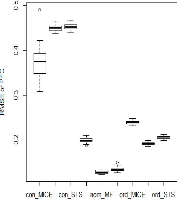
In figure 3.1, 3.2 and 3.3, we use “con” to represent continuous data, “nom” to
Figure 3.1: 5% MI by MICE (left), MF (middle) and STS (right) in COPD data. In continuous data and ordinal data, RMSE is lower in MF method and STS method than that in MICE. In nominal data, PFC is lower in MF method and STS method than that in MICE.
CHAPTER 3. NUMERICAL RESULTS 35
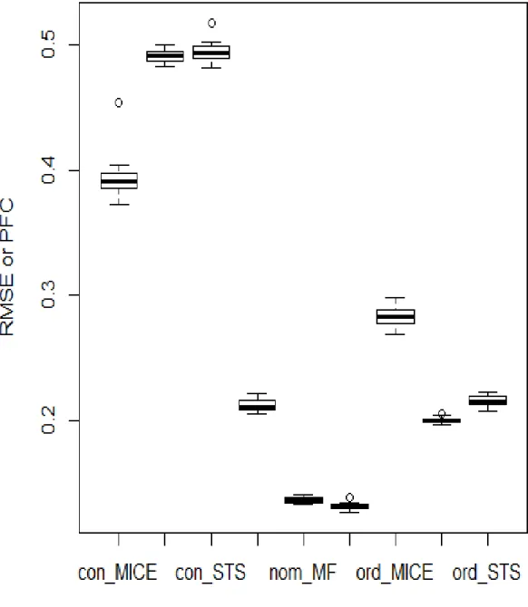
Figure 3.2: 20% MI by MICE (left), MF (middle) and STS (right) in COPD data. In continuous data, RMSE is higher in MF method and STS method than that in MICE. In nominal data, PFC is lower in MF method and STS method than that in MICE. In ordinal data, RMSE is lower in MF method and STS method than that in MICE.
Figure 3.3: 40% MI by MICE (left), MF (middle) and STS (right) in COPD data.In continuous data, RMSE is higher in MF method and STS method than that in MICE. In nominal data, PFC is lower in MF method and STS method than that in MICE. In ordinal data, RMSE is lower in MF method and STS method than that in MICE.
CHAPTER 3. NUMERICAL RESULTS 37
In the comparative study of the imputation methods available for the large
pheno-typic data of COPD, missForest method outperforms MICE method in nominal and
ordinal data types in all missing levels. Merely in the 20% and 40% missing
continu-ous data part of COPD data, MICE does not encounter difficulty in comparison with
missForest. The large variances in MICE limited its application to some real data.
This is consistent with other reports (Stekhoven and Buhlmann (2012) [55]; Jornsten,
et al. (2005) [21]; Kim, et al. (2005) [27]), which illustrate unstable performance of
MICE. In addition, missForest usually was among the state-of-the-art imputation
methods, especially in terms of stability and accuracy. STS method is identified to
be in the top level for imputation in the COPD phenotypic data, if we do not consider
the implementing time.
3.2
Simulation Results
Before simulation research, we discuss why do we use Poisson distribution in our
sim-ulation?
This study focuses on pneumonia. Some pneumonias, such as the Wuhan novel
coro-navirus pneumonia, are diffuse in lung. They have long-term disease characteristics.
For each uninfected or infected individual, we only consider 0 and 1, without
consid-ering any decimals, such as 0.5. Thus, Poisson distribution can be modeled to this
In this subsection, we perform a simulation study of the proposed meta-analysis
method based on random Lasso in the Lasso-Poisson regression model, and compare
it with the random Lasso method based on the Lasso-Poisson regression model in a
separate data set. Consider the equation in a Poisson regression model:
E(Y|X) = eXβ, (3.1)
The simulation data is generated from the model (3.1), where Y has Poisson
distribu-tion. In the mth data set, letx
mi= (xmi,1,· · · , xmi,p)
0
be the observed value of theith
sample. Let ymi be the observed value of the response variable Ymi ∼ P oisson(αm)
of the ith sample in themth data set.
The number of explanatory variables is p = 8, the eight explanatory variables are
pairwise related, and the correlation coefficients of xj1 and xj2 are ρ(xj1, xj2), which
satisfiesρ(xj1, xj2) = 0.5
|j1−j2|. The true values of the explanatory variable coefficients
of the M data sets are all the same, βm = (3,1.5,0,0,2,0,0,0).
To simplify the calculation procedure, in the simulation, the sample size of M = 10
data sets is the same, which is nm = 50. The number of bootstrap samples drawn in
each data set is also the same, which is Bm = 200.
The relative model error (RM E) is depicted below to evaluate the prediction
CHAPTER 3. NUMERICAL RESULTS 39
the true coefficient vector is β0, then the relative model error is defined below:
RM E = ( ˆβ−β
0)0P
( ˆβ−β0)
σ2 , (3.2)
where P
is the covariance matrix of the predictor X, that is P
=Cov(X), that is,
cov(xj1, xj2) = 0.5
|j1−j2|, and σ in the equation (3.2) is the standard deviation of the
error term in the linear model (3.1) (Fan and Li (2001) [14]).
We perform 500 replicates for each example and calculate the average values ofRM E
and ˆβ. To simplify the calculation, we introduce the threshold tn = n1. When the
absolute value of the coefficient estimate of the explanatory variable Xj is greater
than the thresholdtn, the explanatory variable is selected.
We have a meta-analysis method based on the random Lasso in the Lasso-Poisson
regression model and a random Lasso method in the Lasso-Poisson regression model
on a separated dataset. In terms of prediction accuracy and the number of times
of the explanatory variables to be selected, the performance of these two methods
is compared. Besides, the number of selected unimportant explanatory variables is
compared in the simulation. In the cells of the table, the numbers above are from the
meta-analysis, and the numbers in parentheses are from the analysis of the separated
Table 3.1: Coefficient estimate of the important explanatory variables ˆ β1 βˆ2 βˆ5 M1 2.84840 (2.83816) 1.45589 (1.39140) 1.86907 (1.83228) M2 2.88814 (2.88282) 1.42026 (1.37989) 1.86756 (1.85117) M3 2.87732 (2.83076) 1.40564 (1.36609) 1.90109 (1.89337) M4 2.87861 (2.82295) 1.44834 (1.37708) 1.84709 (1.82158) M5 2.87357 (2.84734) 1.37415 (1.35640) 1.91652 (1.85213) M6 2.91475 (2.89460) 1.43756 (1.40661) 1.92419 (1.87455) M7 2.90875 (2.87308) 1.39048 (1.34687) 1.87854 (1.80311) M8 2.90965 (2.89453) 1.41928 (1.38135) 1.87012 (1.80409) M9 2.88199 (2.81149) 1.42789 (1.41138) 2.02593 (1.91989) M10 2.92532 (2.88283) 1.37689 (1.26099) 1.87189 (1.80681)
CHAPTER 3. NUMERICAL RESULTS 41
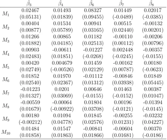
Table 3.2: Coefficient estimate of the unimportant explanatory variables ˆ β3 βˆ4 βˆ6 βˆ7 βˆ8 M1 0.02467 (0.05131) 0.01493 (0.01839) 0.08327 (0.09455) 0.01449 (-0.0489) 0.02017 (-0.0385) M2 0.00404 (0.00877) 0.01534 (0.05789) 0.00941 (0.03165) 0.00515 (0.02440) -0.00132 (0.00201) M3 0.01266 (0.01882) 0.00865 (0.04185) 0.01182 (0.02513) -0.00110 (0.00112) -0.00206 (0.00796) M4 0.00903 (0.02483) -0.00611 (0.01851) -0.01227 (-0.0268) 0.002448 (-0.0245) -0.00357 (-0.0155) M5 0.00420 (0.02749) 0.004679 (-0.00526) 0.01459 (0.02129) -0.00162 (0.00787) 0.00180 (-0.0623) M6 0.01852 (0.02540) 0.01970 (0.02367) -0.01112 (0.01312) -0.00846 (0.03938) 0.01849 (0.05445) M7 -0.01223 (0.01327) 0.0201 (0.03069) 0.00646 (-0.0155) 0.01463 (-0.0152) 0.00387 (0.01047) M8 -0.00559 (0.01679) -0.00064 (-0.00922) 0.01804 (0.03708) 0.00196 (-0.0121) -0.01394 (-0.0145) M9 0.00180 (-0.00212) 0.01094 (0.04778) 0.01845 (0.02576) -0.00255 (0.01231) -0.03232 (0.04227) M10 0.01484 (0.01858) 0.01547 (0.01863) -0.00841 (0.01866) -0.00604 (0.01681) 0.00370 (-0.0186)
Table 3.3: Average RME times 100
M1 M2 M3 M4 M5 M6 M7 M8 M9 M10 RM E 57 (104) 56 (95) 65 (119) 60 (107) 59 (128) 63 (101) 67 (121) 66 (114) 62 (99) 60 (122)
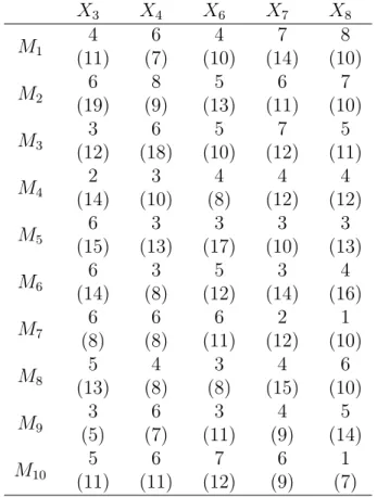
Table 3.4: Numbers of unimportant variables to be selected X3 X4 X6 X7 X8 M1 4 (11) 6 (7) 4 (10) 7 (14) 8 (10) M2 6 (19) 8 (9) 5 (13) 6 (11) 7 (10) M3 3 (12) 6 (18) 5 (10) 7 (12) 5 (11) M4 2 (14) 3 (10) 4 (8) 4 (12) 4 (12) M5 6 (15) 3 (13) 3 (17) 3 (10) 3 (13) M6 6 (14) 3 (8) 5 (12) 3 (14) 4 (16) M7 6 (8) 6 (8) 6 (11) 2 (12) 1 (10) M8 5 (13) 4 (8) 3 (8) 4 (15) 6 (10) M9 3 (5) 6 (7) 3 (11) 4 (9) 5 (14) M10 5 (11) 6 (11) 7 (12) 6 (9) 1 (7)
In Table 3.1 and Table 3.2, we present the estimated value of the important
explana-tory variables and the estimated value of the unimportant explanaexplana-tory variable
coef-ficients. The estimated value obtained by the coefficients based on the meta-analysis
method of random Lasso in multiple data sets is closer to the true coefficient value
than the coefficient estimated value obtained by using the random Lasso method for
multiple data sets respectively. From the averageRM E in Table 3.3, it is pointed out
that the averageRM E obtained by the meta analysis method is smaller. In Table 3.4,
the number of occurrences are summarized when unimportant explanatory variables
are studied in 500 simulations by using these two methods. As can be seen from the
CHAPTER 3. NUMERICAL RESULTS 43
variables is smaller than that of other method. In summary, the performance of the
meta-analysis method of random Lasso has a significant advantage over the predictive
Concluding Remarks
This major paper explores how to handle variable selection in high-dimensional
miss-ing data from two aspects. First, we compared and studied the imputation effects
based on panel data under MICE, missForest, and STS methods. The results show
that MICE, as a non-parametric model, has extremely high time efficiency, and has a
good imputation effect on high missing rate phenotypic data. Although the
missFor-est and STS based on modern statistical learning methods are inferior to MICE in
time efficiency, they usually have better imputation effects. An imputation method
can reduce the bias of the estimated amount caused by missing data. It should be
noted that the method is not a panacea, and different imputation methods are
suit-able for different occasions. Therefore, before performing missing value imputation,
studying the structure of the data can upgrade the effect of the imputation method.
Second, we studied the application of random Lasso in variable selection and combines
it with meta-analysis. In the count data sets of the Lasso-Poisson regression model,
CHAPTER 4. CONCLUDING REMARKS 45
the estimated coefficients of the explanatory variables based on the meta-analysis
method of random Lasso in multiple data sets are better than those of separated
data sets. The coefficient estimate based on the meta-analysis method should be
closer to the true coefficient value, and the effect of removing unimportant variables
is significant. Even when multiple explanatory variables are highly correlated, the
meta-analysis method based on random Lasso in multiple data sets still has good
predictions.
There are at least five aspects of novelty in this study. First, this is a systematic
com-parative study of approaches for estimating missing values for large-scale phenotypic
data. We compare the three existing methods (missForest, multivariate imputation
by chained equations (MICE) and self-training selection (STS)). Second, we indicate
missForest and STS significantly impute the correct missing values for each data type
in a given data set, though STS selection method is time-consuming. Third, we
illus-trate the importance of variable selection by using random lasso method in a discrete
model simulation. Fourth, we use meta-analysis to further analyze high-dimensional
data sets. Fifth, MFRL approach is firstly illustrated as a principled method of
ad-dressing variable selections in high-dimensional incomplete data.
In conclusion, we suggest missForest for imputation and random Lasso for variable
selection in high-dimensional incomplete data (Liu, et al. (2016)[38]). We name this
method as MFRL. However, further investigations are needed. This work should
[1] Hirotugu Akaike. (1973). Information theory and the maximum likelihood
princi-ple in 2nd International Symposium on Information Theory (B.N. Petrov and F.
Cs ¨a ki, eds.). Akademiai Ki `a do, Budapest.
[2] Rebecca Andridge, Roderick Little. (2010). A Review of Hot Deck Imputation for
Survey Non-response. International Statistical Review, Volume 78, 40-64
[3] Orley Ashenfelter, William Peirce. (1966). Industrial Conflict: The Power of
Pre-diction. ILR Review, Volume 20, 92-95
[4] Francis Bach. (2008). Bolasso: model consistent lasso estimation through the
bootstrap. Proceedings of the 25th international conference on Machine learning,
ACM, 33–40.
[5] Avrim L. Blum, Pat Langley. (1997). Selection of relevant features and examples
in machine learning. Artificial Intelligence, Volume 97, 245-271
[6] Leo Breiman. (2001). Statistical Modeling: The Two Cultures (with comments
and a rejoinder by the author). Statistical Science, Volume 16, 199-231
BIBLIOGRAPHY 47
[7] Guy Brock, John Shaffer, Richard Blakesley, Meredith Lotz, George Tseng .
(2008). Which missing value imputation method to use in expression profiles:
a comparative study and two selection schemes. BMC Bioinformatics, Volume 9,
1-12
[8] Emmanuel Candes, Terence Tao. (2007). The Dantzig selector: Statistical
estima-tion when p is much larger than n. Statistica Sinica, Volume 35, 2313-2351
[9] William Cochran. (1977). Sampling Techniques. John Wiley & Sons, New York
[10] Brenda Cox, Steven Cohen. (1983). Methodological issues for health care surveys.
Marcel Dekker Inc., New York
[11] Edward Deming. (1944). On Errors in Surveys. American Sociological Review,
Volume 9, 359-369
[12] Edwards Deming, Frederick Stephan. (1940). On a Least Squares Adjustment of
a Sampled Frequency Table When the Expected Marginal Totals are Known.The
Annal