Priors for Bayesian Shrinkage and High-Dimensional Model Selection

(1)

PRIORS FOR BAYESIAN SHRINKAGE AND HIGH-DIMENSIONAL MODEL SELECTION

A Dissertation by MINSUK SHIN

Submitted to the Office of Graduate and Professional Studies of Texas A&M University

in partial fulfillment of the requirements for the degree of DOCTOR OF PHILOSOPHY

Chair of Committee, Valen E. Johnson Co-Chair of Committee Anirban Bhattacharya Committee Members, Jianhua Huang

Byung-Jun Yoon Head of Department, Valen E. Johnson

August 2017

Major Subject: Statistics

(2)

ABSTRACT

This dissertation focuses on the choice of priors in Bayesian model selection and their applied, theoretical and computational aspects. As George Box famously said “all models are wrong, but some are useful"; many statisticians and scientists are aware of the importance of model selection. In a Bayesian perspective, however, it is challenging to choose the prior on the parameters involved in model selection or how to evaluate the criterion on the prior, especially when the number of models to be compared is massive or when a nonparametric model is considered.

For high-dimensional Bayesian model selection for linear models, my dissertation studies theoretical perspectives of the choice of the prior on the regression coefficient. Especially, I consider the nonlocal prior densities that assign zero density around the null value, which is typically 0 in model selection settings. When certain regularity conditions apply, I demonstrate that the model selection procedure based on the nonlocal priors is consistent for linear models even when the number of covariates pincreases sub-exponentially with the sample size n. I investigate the asymptotic form of the marginal likelihood based on the nonlocal priors and show that it attains a unique penalty term that adapts to the strength of signal corresponding variable in the model, and I remark that this term cannot be attained from local priors such as Gaussian prior densities.

Another topic of my dissertation is about computational aspects of Bayesian model selec-tion under high-dimensional settings. A full posterior sampling using existing Markov chain Monte Carlo (MCMC) algorithms to explore high-dimensional model space is highly ineffi-cient and often not feasible from a practical perspective. To overcome this issue, I propose a scalable stochastic search algorithm called Simplified Shotgun Stochastic Search with Screen-ing (S5), which efficiently explores the model space. The S5 algorithm dramatically reduces

(3)

the computational burden to search the neighborhood of a model by considering a screening step within the algorithm. Its empirical performance is examined in several examples, and it outperforms existing algorithms in the sense that S5 is computationally fast while it efficiently searches the model space. S5 is used to implement the model selection procedures introduced in this dissertation, including linear and nonparametric model selection. The computing func-tions are provided in theRpackageBayesS5inCRAN(https://cran.r-project.org).

For nonparametric regression models, I introduce a new shrinkage prior on function spaces, the functional horseshoe prior, that encourages shrinkage towards parametric classes of func-tions. When the true underlying function is in the parametric class, improved estimation per-formance is obtained relative to classical nonparametric procedures. The proposed prior also provides a natural penalization interpretation, and casts light on a new class of penalized like-lihood methods for function estimation. I theoretically exhibit the efficacy of the proposed approach by showing an adaptive posterior concentration property.

The last topic of the dissertation is about a novel extension of the nonlocal idea to functional spaces, called the nonlocal functional prior, which is suitable for nonparametric Bayesian hy-pothesis testing (model selection) problems. I illustrate the asymptotic rate of the Bayes factor defined by the proposed prior for nonparametric hypothesis testing problems. I apply the pro-posed prior densities for high-dimensional model selection of nonparametric additive models, and investigate the model selection consistency of the resulting model selection procedure. I provide some simulation studies and real data examples that show that the proposed model selection procedure outperforms state-of-the-art methods in finite samples.

(4)

DEDICATION

(5)

ACKNOWLEDGMENTS

First of all, I would like to express my deep gratitude to my advisors Valen E. Johnson and Anirban Bhattacharya. Because of their thoughtful advice, I was able to complete my dissertation, and they helped me a lot to grow academically. Val taught me the right attitude and passion towards science and he has alway given me a piece of warm hearted advice. Anirban is not only a good friend, but he is also a good partner to discuss ideas. Val and Anirban, I have been incredibly inspired by you, and no word of thanks is enough for your wonderful mentorship.

I would also like to extend my gratitude to the members of my dissertation committee, Dr. Jianhua Huang and Dr. Byung-Jun Yoon for their support and encouragement. Thanks also to Dr. Irina Gaynanova and Dr. Xianyang Zhang for giving me helpful advice to apply for academic jobs and to improve my presentation skills. Dr. David Rossell has been extremely encouraging and I have thoroughly enjoyed the discussions with him. It has been a great pleasure working with Dr. Naveen N. Narisetty, even though our work has been delayed so long. I believe that we can finish the project soon. Amir Nikooienejad is also a good friend of mine, and I really appreciate his constant encouragement. I am also grateful to my friend Sangyoon Yi for buying me Starbucks coffee many times.

Dr. Ersen Arseven, who has worked in the clinical trial industry for 30 years, has been a good mentor. He gave me a lot of supports and warm-hearted advice. In particular, his advice for presentation and job interview was really useful and practical.

Finally, I devote my dissertation to my family: my beloved wife Mirae, my daughter Jane, my son Sungmin (Daniel), my parents and my parents-in-law. Especially, my mother Eulsun Kim and my mother-in-law Soonja Lee crossed the Pacific Ocean from South Korea and came to America to help us when my daughter and son were newborn. I would also like to thank my

(6)

grandmother and grandfather for their dedicated support. Without supports from my family, none of this work would have been possible. I love you!

(7)

CONTRIBUTORS AND FUNDING SOURCES

Contributors

This work was supported by a dissertation committee consisting of Dr. Valen E. Johnson (co-advisor), Dr. Anirban Bhattacharya (co-advisor) and Dr. Jianhua Huang of the Department of Statistics and Dr. Byung-Jun Yoon of the Department of Electrical Engineering.

All other work conducted for the dissertation was completed by the student independently. Funding Sources

Graduate study was supported by a teaching assistantship from Texas A&M University and from the National Institute of Health (NIH) R01 CA.

(8)

2. NONLOCAL PRIOR DENSITIES FOR HIGH-DIMENSIONAL LINEAR MODEL SELECTION . . . 19

2.1 Introduction . . . 19

2.2 Nonlocal Prior Densities for Regression Coefficients . . . 21

2.3 Numerical Results . . . 24

2.3.1 Simulation Studies Using Precision-Recall Curves . . . 24

(9)

2.4 Model Selection Consistency . . . 31

2.5 Connections Between Nonlocal Priors and Reciprocal Lasso . . . 33

2.6 An Adaptive Form of Asymptotic Marginal Likelihoods Based on Nonlocal Priors . . . 35

2.7 Real Data Analysis . . . 36

2.7.1 Analysis of Polymerase Chain Reaction (PCR) data . . . 36

2.7.2 A Simulation Study Based on the Boston Housing Data . . . 39

2.8 Conclusion . . . 41

3. SIMPLIFIED SHOTGUN STOCHASTIC SEARCH WITH SCREENING ALGO-RITHM FOR HIGH-DIMENSIONAL BAYESIAN MODEL SELECTION . . . 44

3.2 Shotgun Stochastic Search Algorithm (SSS) . . . 44

3.3 Simplified Shotgun Stochastic Search Algorithm with Screening (S5) . . . 45

3.4 Performance Comparisons Between S5 and SSS . . . 47

3.4.1 Application to Real Data Examples . . . 49

3.5 RPackage: BayesS5 . . . 51

3.5.1 S5Function . . . 51

3.5.2 S5_parallelFunction for Parallel Computing Environments . . . . 55

4. FUNCTIONALHORSESHOEPRIORFORNONPARAMETRICSUBSPACE AGE . . . 58

4.2 Preliminaries . . . 60

4.3 Functional Horseshoe Prior . . . 61

4.3.1 Posterior Concentration Rate . . . 65

4.4 Simulation Studies for Univariate Examples . . . 68

4.5 Applications to Additive Models . . . 73

4.5.1 A Comparison to the Standard Horseshoe Prior . . . 74

4.5.2 Simulation Studies . . . 75

4.5.3 Real Data Analysis: Boston Housing Data and Ozone Data . . . 79

4.6 Conclusion . . . 82 SHRINK

(10)

5. NONLOCAL FUNCTIONAL PRIORS FOR NONPARAMETRIC HYPOTHESIS

TESTING AND HIGH-DIMENSIONAL MODEL SELECTION . . . 83

5.2 Bayesian Nonparametric Hypothesis Testing Procedures . . . 86

5.3 Convergence Rates of Bayes Factor . . . 90

5.3.1 Preliminaries . . . 90

5.3.2 Local Priors . . . 90

5.3.3 Moment Functional Prior Densities . . . 92

5.3.4 Inverse Moment Functional Prior Densities . . . 94

5.3.5 The Choice ofKn . . . 95

5.4 Examples of Bayesian Hypothesis Tests Using Nonlocal Functional Priors . . . 95

5.5 Nonparametric Additive Model Selection Using Nonlocal Functional Priors . . 99

5.5.1 Additive Model Selection Consistency for High-dimensional Settings . 102 5.5.2 Asymptotic Rates of Marginal Likelihood for Additive Models . . . 104

5.5.3 Computational Strategy Using S5 . . . 106

5.5.4 Simulation Studies . . . 107

5.5.5 Practical Selection of Hyperparameter Values . . . 114

5.6 Applications to Real Data Sets . . . 116

5.6.1 Bardet-Biedl Syndrome Gene Expression Data . . . 116

5.6.2 Near Infrared Spectroscopy Data . . . 116

5.6.3 Technical Details and Results . . . 116

5.7 Conclusion . . . 118

REFERENCES . . . 119

APPENDIX A. PROOFS OF THEORETICAL RESULTS . . . 130

A.1 Nonlocal Prior Densities for High-dimensional Linear Model Selection . . . 130

A.2 Functional Horseshoe Prior for Nonparametric Subspace Shrinkage . . . 149

A.3 Nonlocal Functional Priors for Nonparametric Hypothesis Testing andHigh-dimensionalModelSelection . . . 160

(11)

B.1 Nonlocal Prior Densities for High-dimensional Linear Model Selection . . . 176 B.2 Functional Horseshoe Prior for Nonparametric Subspace Shrinkage . . . 177 B.3 Nonlocal Functional Priors for Nonparametric Hypothesis Testing

and High-dimensionalModelSelection . . . 179 B.3.1 Modified Simplified Shotgun Stochastic Search with Screening (S5) for

Additive Models . . . 179 B.3.2 Laplace Approximations of Marginal Likelihoods Based on Nonlocal

(12)

LIST OF FIGURES

2.1 Nonlocal prior density functions for a single regression coefficient . . . . 22

2.2 Plot of the mean precision-recall curves over 100 datasets. . . 28

2.3 Averaged posterior true model probability and the number of models which attain the posterior odds ratio, with respect to the maximum a posteriori model, larger than0.001. . . 29

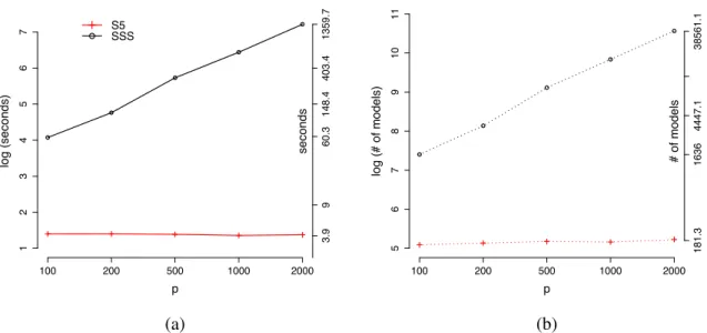
3.1 Performance comparison between S5 and SSS. (a) Average computation time to first find the MAP model; (b) Average number of models searched before hitting the MAP model. . . 48

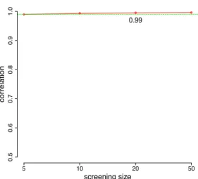
3.2 Correlation between the top 10 posterior model probabilities estimated from SSS and S5 with different screening set sizes. . . 49

3.3 Marginal inclusion probabilities approximated by S5 for the synthesized Boston housing data set. . . 54

4.1 A description of the prior density of !. The first two columns illustrate the prior density function of!with different hyperparameters(a, b) . . . 64

4.2 Examples when the underlying true functions are parametric. . . 71

4.3 Examples when the underlying true functions are nonparametric. . . 72

4.4 Performance comparison with simulated data sets. . . 78

5.1 The convergence rate of Bayes factor under a true null. . . 97

5.2 Performance of additive model selection (1): the results of Scenario 1 and Scenario 2. . . 111

5.3 Performance of additive model selection (2): the results of Scenario 3 and Scenario 4 . . . 112

5.4 A description of the hyperparameter selection procedure. The black line and the blue line are the density functions of the null and the prior distribution of FT_(I _Q 0)F/b2, respectively, for a given⌧nandb2 . . . 115

ate

(13)

LIST OF TABLES

2.1 Optimal hyperparameters for Bayesian model selection methods . . . 30

2.2 Analysis of the PCR data. . . 39

2.3 The Boston Housing data set. . . 40

3.1 Comparisons between S5 and SSS using the Bardet-Biedl syndrome data and the Boston housing data. . . 50

4.1 Results of univariate examples . . . 69

4.2 Results of real data examples . . . 81

5.1 The convergence rate of Bayes factor under true alternative hypotheses. . . 98

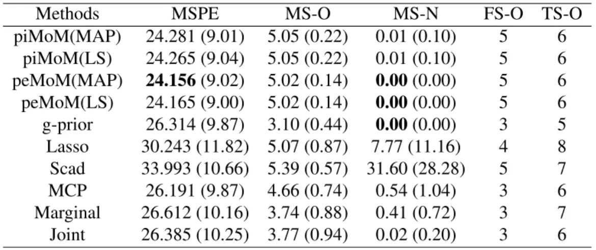
5.2 Optimal MSE and MSPE of each method for the considered settings. . . 110

5.3 Real data examples for additive model selection. . . 117

- .

(14)

-1. INTRODUCTION

1.1 A Brief Review of Bayesian Model Selection

Suppose that a set of H modelsM = {M1, . . . , MH}is considered for observed data y.

Under a modelMh 2 M, the density function ofyis L(y | ✓h, Mh), where✓h is a vector of unknown parameters under modelMh. For Bayesian inference, priors should be fully specified by assigning a prior distribution⇡(✓m |Mh)to the parameters of each model and a model prior

⇡(Mh)to each model. The posterior probability of modelMh conditionally on the observedy can be expressed as ⇡(Mh |y) = _PmMh(y)⇡(Mh) h0mMh0(y)⇡(Mh0) , (1.1) where mM_h(y) = Z L(y_|✓h, Mh)⇡(✓h |Mh)d✓h

is the marginal likelihood of a modelMh. Based on these posterior model probabilities, pair-wise comparison of modelsM1andM2is conducted by the posterior odds that can be expressed

as a product between the ratio of marginal likelihoods and the model prior odds; i.e.,

⇡(M1 |y) ⇡(M2 |y) = mM1(y) mM2(y) ⇥ ⇡(M1) ⇡(M2) .

In particular, the ratio of marginal likelihoodsmM1(y)/mM2(y)is called theBayes factor

and it determines the decision rules for Bayesian hypothesis testing problems as discussed in Kass and Raftery (1995) and Jeffreys (1961). The higher the Bayes factor value supports, the more evidence in favor of M1. In Kass and Raftery (1995), a rough descriptive statement of

(15)

some decision rules regarding Bayes factors was empirically addressed as

logBF10 Evidence againstH0

0to1 Not worth more than a bare mention 1to3 Positive

3to5 Strong >5 Very strong.

More discussions and empirical examples regarding Bayes factor are provided in Kass and Raftery (1995).

Throughout this dissertation, I assume that one of considered models is the true model that represents the data-generating process, which is a setting called the “M-closed" framework as proposed in Bernardo and Smith (1994). This in itself is somewhat controversial, because the true model might not exist or it might not be one of those under consideration. However, it is a helpful viewpoint for at least thinking through the consequences of a true Bayesian model selection procedure and desirable qualities.

I now introduce a desirable asymptotic property for Bayesian model selection procedures calledmodel selection consistencythat can be defined as follows.

Definition 1. (Model Selection Consistency) Suppose thattis the true data-generating model. Then, if

⇡(t_|y)_!p 1,

asn _{! 1}, the Bayesian model selection procedure is called “consistent".

From a theoretical point of view, when the number of models is fixed regardless of the sample size n, Schwarz (1978) showed that the model selection procedures defined by some general classes of priors; e.g. Gaussian priors achieve the model selection consistency.

(16)

How-ever, when I allow the number of models to increase at a certain rate of n, the asymptotic behavior of the posterior probability of the true model is not clear. This situation is commonly faced in high-dimensional variable selection problems for regression models due to the fact that the total number of models for variable selection is2p_{, where} _p( _n)_{is the total number} of variables .

For the Bayesian framework, the uncertainty of the model space can be represented by the posterior model distribution ⇡(M1 | y), . . . ,⇡(MH | y). By considering ⇡(Mh | y) as

a measure of the "truth" of modelMh, a natural strategy for model selection is to choose the model that attains the largest posterior model probability. This model is called themaximum a posteriori(MAP) model, i.e. McM AP _{= argmax}

h⇡(Mh | y). These posterior probabilities are also important for full posterior inference in prediction using Bayesian model averaging

(Raftery et al., 1997), which is quantified by the posterior predictive distribution as p(ypred _|

y) =P_h0⇡(ypred |Mh0,y)⇡(Mh0 |y)for a future observationypred.

1.1.1 Bayesian Model Selection for the Linear Regression Model

Consider the standard setup of a Gaussian linear regression model with a univariate re-sponse andpcandidate predictors. Lety = {y1, . . . , yn}T denote a vector of responses for n

individuals andX ann⇥pmatrix of covariates. Let ={ 1, . . . , p}Tdenote the regression coefficients. The linear regression model for the data is given by

y=X +✏, (1.2)

where✏⇠Nn(0, 2_{In). However, in high-dimensional settings (n} _⌧_{p), the unique MLE does}

not exist and a MLE fails to achieve consistency of estimation. To overcome this issue, from a Bayesian perspective, one can consider a sparsity inducing prior (Castillo et al., 2015) that restricts the size of a given modelkand puts zero prior probability on other parameters that are

(17)

not in modelk. More precisely, for a given modelk, the prior is

⇡( _|k)_/⇡k( k) 0( kc) (1.3)

where the term 0( kc) implies the coordinates _kc = { _j : j 2 kc} being zero and ⇡k( _k)

is a prior on the nonzero regression coefficients k = { j : j 2 k}. This class of priors includes many instances such as Zellner’sg-prior (Zellner, 1986), mixtures of g-priors (Liang et al., 2008) and discrete mixtures of spike and slab priors (Ishwaran and Rao, 2005). With a slight abuse of the notation, I denote the prior on the model space as ⇡(k)for a model k.

By following the definition of the posterior model probability in (1.1), the resulting posterior probability of modelkis defined as

⇡(k_|y) = Pmk(y)⇡(k)

lml(y)⇡(l)

,

where the marginal likelihood of a modelkis given by

mk(y) = Z

L(y_| ,k)⇡( _|k)d ,

for the likelihood function for modelk, L(y | ,k). More practically, when 2 _{is unknown,}

a prior on 2 _{can be deployed and the corresponding marginal likelihood can be defined by}

integrating with respect to the prior on 2_{. The posterior model probability can be used to select}

variables that are associated with the response. The simplest approach to the best model is to consider the MAP model that maximizes the posterior model probability. An other option is to utilize the marginal inclusion probabilities{qj :j = 1, . . . , p_}, whereqj =P_k:_j₂_k⇡(k_|y)for j = 1, . . . , p. The median probability model is defined as the set of variables whose marginal inclusion probability is larger than 0.5. Barbieri and Berger (2004) showed that the median probability model is optimal in a predictive sense when only a single model is considered .

(18)

Some desirable theoretical properties of the posterior inference with some choices of the prior specification (1.3) have been discussed in high-dimensional settings. Johnson and Rossell (2010) proposed a class of prior densities callednonlocal prior densitiesfor⇡k( k|k).

Nonlo-cal prior densities are density functions that are identiNonlo-cally zero whenever a model parameter is equal to its null value, which is typically 0 in model selection settings. More formal definition is as follows:

Definition 2. Suppose that✓is a parameter supported in⇥and✓0 is the null value. Consider

a hypothesis test H0 : ✓ = ✓0 versus H1 : ✓ 6= ✓0. Under the alternative hypothesis, a

prior density⇡ is nonlocal, if for every✏>0, there is > 0such that⇡(✓) <✏for all✓ ₂⇥ such that_|✓ ✓0_|< .

Conversely, local prior densities are positive at the null parameter value. In Johnson and Rossell (2012), it was shown that Bayesian model selection procedures based on nonlocal priors achieve model selection consistency when p = O(n). However, when p increases at a sub-exponential rate of n, i.e. logp = O(nc₎ _{for some} ₀ _ _{c <} _{1, its posterior model} consistency has not been derived.

Also, under increasingpat a sub-exponential rate ofn, Narisetty and He (2014) investigated the asymptotic behavior of model selection procedure based on a Gaussian prior with diverging variance as n grows. Castillo et al. (2015) discussed some general conditions on priors on the coefficient and models for the optimal rate of posterior contraction and model selection consistency. All priors considered in the literature were local priors.

1.1.2 Bayesian Model Selection in the Nonparametric Regression

Consider a simple nonparametric regression model defined according to a response y =

{y1, . . . , yn}and a univariate predictorX ={x1. . . , xn}

(19)

where✏ _⇠ N(0, 2_I

n)andF = {f(x1), . . . , f(xn)}with the unknown regression functionf. From a practical point of view, a practitioner should decide whether the shape off is specified by a parametric from such as linear or quadratic function, or a nonparametric representation using splines, wavelet, Gaussian processes etc. This argument can be formalized as a model selection problem by writing

H0 :F 2L versus H1 :F 62L, (1.5)

whereLis a class of the parametric functions that are specified in advance. For example, if a practitioner is interested in whetherF is linear or not,Lcan be defined asL = { 0 + 1X : 0, 1 2 R}. Under H0, the resulting model is simply a univariate linear regression model.

UnderH1, one can model the unknown functionf as spanned by a set of pre-specified basis

functions{ j}1jKn, whereKnis the number of basis functions, as follows:

f(x) = Kn X

k=1

k k(x). (1.6)

I shall work with the B-spline basis (De Boor, 1978) in the sequel, although the method-ology generalizes to a larger class of basis functions. The B-splines basis functions can be constructed in a recursive way. Let the positive integer q denote the degree of the B-spline basis functions satisfyingKn > q+ 1. Without loss of generality, assume thatxi ₂ [0,1]for i = 1, . . . , n. Define a sequence of knots0 = t0 < t1 <· · ·< tKn q = 1. In addition, define

(20)

(1978), the B-spline basis functions are defined as k,1(x) = 8 > > < > > : 1, tk x < tk+1, 0, otherwise, k,q+1(x) = x tk tk+q tk k,q(x) + tk+q+1 x tk+q+1 tk+1 k+1 ,q(x),

fork= q, . . . , Kn q 1. I reindexk = q, . . . , Kn q 1tok= 1, . . . , Knand the number of basis functions isKn. Letting = ( 1, . . . , Kn)

T denote the vector of basis coefficients

and = _{ k(xi)_}1in,1kKn denote then⇥Knmatrix of basis functions evaluated at the

observed covariates, I modelF = .

Even though parametric models might fail to capture important features of the data when they do not fit into the parametric form, the asymptotic behavior of the parametric model is superior to the nonparametric counterparts when the data-generating model is in the class of the parametric models or it is close enough to the class. In Ghosal and van der Vaart (2007), it was shown that the contraction rate of the posterior distribution defined by isotropic Gaussian priors for the nonparametric regression model in (1.4) isn ↵/(1+2↵)_{, where}_↵ _>₀_{quantifies the}

smoothness of the function, which is slower than the parametric optimal raten 1/2_{. In practice,}

nonparametric models also require extra steps to choose the tuning parameter that controls the smoothness of the estimated function, and they are usually challenging in computational and practical senses. Furthermore, in many cases, parametric shapes of F have advantages for interpretation of the regression function. For example, the slope parameter of the linear regression model represents the linear association between the response and the covariate.

In the Bayesian paradigm, the evidence in favor of each model in (1.5) is naturally quanti-fied by Bayes factor that was introduced in Jeffreys (1961) and defined as

BF10=

m1(y)

m0(y)

(21)

wherem1(y)andm0(y)are the marginal likelihoods underH1andH0; i.e. m1(y) = R

L(y_|

, H1)d⇡N P( ) and m0(y) = R

L(y _| ✓, H0)d⇡P(✓), where ⇡N P is a prior on the B-spline coefficient and⇡P is a prior on the parameter✓2Rd0 for the parametric model inL.

For the hypothesis test in (1.5), Choi et al. (2009) considered a semiparametric model that has an additive form between a parametric function and a nonparametric function. They investigated the asymptotic behavior of the Bayes factor defined by Gaussian priors on the coefficients of the basis functions. More general theoretical results regarding Bayes factor were provided in Choi and Rousseau (2015), which showed that the resulting Bayes factor achieves consistency in the sense that BF10 converges to zero in probability when the true

data-generating process supportsH0 andBF10diverges to infinity in probability, otherwise.

When multiple predictors are considered, the nonparametric additive model (Hastie and Tibshirani, 1986) can be considered, which is expressible as

y=

p

X

j=1

fj(Xj) +✏, (1.7)

where ✏ ⇠ N(0, 2_In) _and _fj _{is the} _{j-th marginal regression function. Also,} _Xj _{is the} _j-th

covariate among pcovariates. The setting for (1.4) can be naturally extended to the additive model by modeling each component function as a linear combination of the B-spline basis functions, i.e. fj(Xj) = PKk=1n k(Xj) jk = j j, where j = { j1, . . . , jKn} and j = { 1(Xj), . . . , Kn(Xj)}for1j p. Similar to the model selection procedures discussed in

Section 1.1.1 for linear models, I am interested in selecting variables that are associated with the responsey, and the uncertainty identification of the model space is also my concern.

From a frequentist perspective, there have been several studies regarding the additive model selection in high-dimensional settings, including Ravikumar et al. (2009), Meier et al. (2009), and Huang et al. (2010). Many procedures use the group Lasso penalty proposed in Yuan and Lin (2006) to induce the sparse representation of the component function. Theoretical

(22)

proper-ties of associated estimation and model selection properproper-ties have been investigated in Raskutti et al. (2012) and Yuan and Zhou (2016). In Bayesian frameworks, Shang and Li (2014) consid-ered the Bayesian additive model in high-dimensional settings and provided some conditions on the prior on the basis coefficient necessary to achieve model selection consistency. How-ever, in Shang and Li (2014), the practical guideline regarding the choice of prior on the spline coefficients is unclear, and the computational challenges are not resolved, since the proposed algorithm is based on an MCMC algorithm that is inefficient in high-dimensional settings. 1.2 Research Challenges and Main Contributions

1.2.1 Linear Model Selection in High-dimensional Settings The Choice of Priors

For high-dimensional linear model selection problems, there is a rich literature regarding the choice of prior on the regression coefficient and the model space. In Castillo et al. (2015), a class of model priors calledcomplexity priorswas defined as

⇡(k)_/ ✓ p |k| ◆ 1 a |k|p b|k|,

for some constants a, b > 0. I note that the Bernoulli-uniform prior discussed in Scott and Berger (2010),⇡(k)/ _|kp|

1

, is a special case of the complexity prior witha= 1andb = 0. Castillo et al. (2015) provided tail conditions on the prior on the coefficients and sufficient conditions on the hyperparameter of a class of model priors to guarantee the optimal posterior concentration rate and model selection ocnsistency. Narisetty and He (2014) investigated the asymptotic behavior of model selection procedures based on the Bernoulli-uniform model prior and a Gaussian prior with variance that increases faster thanp2+✏_{for any small}_✏_>_0.

For linear models, the posterior model probability based on priors discussed in Castillo et al. (2015) and Narisetty and He (2014) (or Zellner’sg-prior Zellner (1986)) can be asymptotically

(23)

expressed as

log⇡(k_|y)_⇡lk(bk) |k|cn,p+C, (1.8)

wherelk is the logarithm of the likelihood function under a modelkand bk is the maximum

likelihood estimator of kunder modelkfor some sequencecn,p>0and a constantC. For ex-ample, as shown in Narisetty and He (2014), if k |k⇠N(0, pc)for some constantc >0and

the Bernoulli-uniform prior is imposed on the model space, then the logarithm of the resulting posterior model probability is asymptotically equivalent tolk(bk) (1 +c/2)|k|logp+C. It

is interesting to note that this expression is exactly the same as penalized likelihood procedures with aL0penalty (e.g., Zhang et al. (2010), Chen and Chen (2008), Kim et al. (2012)).

The main property of the form in (1.8) is that the penalty strength on modelkis determined

solely by its size |k_|, regardless of the marginal strength of the regression coefficient in the

model. For example, suppose that two different models with the same model size are consid-ered. One model consists of predictors that are strongly associated with the response, and the other model contains only some of strongly associated variables and the rest of variables in the model are weakly associated with the response. Under objective function in (1.8), two models would be penalized by the same amount, because the model size is the same. Even though the model with weakly associated variables will be strongly penalized by the log-likelihood func-tion, the model selection criterion with the penalty that only depends on the model size might not be able to select important variables and might fail to control the multiplicity in a practical sense since there are too many models to be compared in the model space in high-dimensional settings.

In this dissertation, certain sufficient conditions on the nonlocal priors defined in Defini-tion 2 will be provided to allow the resulting model selecDefini-tion procedure to achieve the model selection consistency whenlogp = O(nc₎ _{for some}₀ _ _{c <} _{1. Also, the asymptotic form}

(24)

of the posterior model probability defined by the nonlocal priors will be discussed, and I will point out that the asymptotic form of the posterior model probability contains a unique form of penalty on the regression coefficient. The form of penalty cannot be attained by local priors that have been used previously in the literature.

The asymptotic form of the logarithm of the posterior model probability defined by the nonlocal prior on the regression coefficients can be expressed as

log⇡(k_|y)_⇡lk(bk) |k| X j=1 ⌧ e2 k,j + log⇡(k) +C0, (1.9)

where e_k_,j = bk,j+Op (n/⌧) 1/4 and⌧ is the hyperparameter for the nonlocal prior, which controls the parsimony of model selection. Also, b_k_,j_{denotes the}_{j-th element of} b_k_.

While model selection procedures defined by local priors penalize a model only by the size of the model, the penalty P|k|

j=1⌧/ek2,j in the objective function in (1.9) is adaptively determined by the strength of the marginal signal that is measured by the e2

k,jterm and imposes different penalties on each predictor in the given model. This adaptive term encourages the model selection procedure to select variables with strong signals. This property has not been previously discussed in the original literature (Johnson and Rossell, 2010), and it explains why the nonlocal prior shows empirically outstanding performance in model selection.

A Scalable Computation

Even though sparsity inducing priors in (1.3) enjoy desirable theoretical properties, the practical implementation of Bayesian model selection procedures based on these priors is computationally challenging due to the discrete nature of the prior. Since the total number of possible models is enormous (2p_{) even for a moderate dimension}_{p, it is not computationally} practical to calculate all possible marginal likelihoods to evaluate the exact posterior model probabilities. Thus, algorithms to efficiently explore the model space to reduce the

(25)

computa-tional burden are needed. One might consider reversible jump Markov chain Monte Carlo pro-posed in Green (1995) for posterior inference, but that algorithm is inefficient and impractical, especially in high-dimensional settings. A Gibbs sampling based algorithm called the Stochas-tic Search Variable Selection (SSVS) was proposed in George and McCulloch (1993), but its computational efficiency decreases as the number of predictors increases. Besides Markov Chain Monte Carlo (MCMC) approaches, Hans et al. (2007) introduced Shotgun Stochastic Search (SSS) to efficiently search the model space and approximate posterior model probabili-ties. However, the computational demands of SSS significantly increases as dimension grows. More recently, some deterministic approaches, such as Rockova and George (2014) and Car-bonetto and Stephens (2012), were used to find the MAP model. Those algorithms only find a single model and do not provide posterior model probabilities, so it is challenging to quantify the uncertainty on the model space.

To ameliorate these computational issues, several continuous shrinkage priors have been proposed, including the Bayesian Lasso (Hans, 2009; Park and Casella, 2008), the horseshoe prior (Carvalho et al., 2010), the generalized double Pareto shrinkage prior (Armagan et al., 2013) and the Dirichlet-Laplace prior (Bhattacharya et al., 2015). Those priors can be ex-pressed as scale mixtures of Gaussian distributions, so the resulting marginal priors are con-tinuous. By avoiding the structure of the discrete mixtures, those continuous shrinkage priors provide a computational advantage, and efficient MCMC algorithms are available for sampling from the corresponding posterior distribution; e.g. Bhattacharya et al. (2016). However, pos-terior inferences obtained under these continuous priors do not induce any pospos-terior model probabilities. Nor is it straightforward to choose a model or select variables.

In this dissertation, a scalable stochastic model search algorithm calledSimplified Shotgun Stochastic Search with Screening(S5) is proposed, and its empirical performance is examined. S5 is a simplified version of SSS and it utilizes a screening step embedded in the algorithm to reduce the model space to be searched. Even though S5 is motivated by SSS, its efficiency

(26)

in searching interesting regions in the model space is remarkably improved by adopting a screening algorithm. For linear model selection in high-dimensional settings, the S5 algorithm often finds the MAP model hundreds of times faster than SSS does, but it identifies the same MAP model as SSS in all data sets examined in this dissertation. Furthermore, S5 accurately approximates posterior model probabilities and approximated posterior model probabilities are almost identical to those obtained from SSS. This algorithm is applicable to any variable selection procedures as long as a sound screening procedure is available. That is, it can be used for logistic regression models and nonparametric additive models. I extend the S5 algorithm to search the space of nonparametric additive models by adding a nonparametric screening step in the algorithm, and used it to implement the nonparametric model selection procedure that is described in the following sections.

An R functions that implements S5 is available in the R package BayesS5 in CRAN (https://cran.r-project.org). This package includes a parallelized version of the code, which lets multiple independent chains search the model space simultaneously. This al-lows the algorithm explore a wider range of interesting regions in the model space. Simple tutorials about the package are also provided in this dissertation.

1.2.2 Nonparametric Model Selection in High-dimensional Settings A Novel Shrinkage Prior for Nonparametric Regression

Frequently, practitioners face the problem of choosing between a parametric model and a nonparametric model, where the parametric model is nested within a more general class of functions. For example, a simple linear regression model or a nonparametric regression model might be considered for a data set, and the linear regression model is a special case of the nonparametric model. However, sometimes building a reasonable criterion for the choice between the parametric form and nonparametric form of the function is not evident, especially when multiple functions are involved in the model.

(27)

From a frequentist perspective, there has been a surge of interest in solving this problem us-ing various forms of penalized estimation via the group Lasso (Yuan and Lin, 2006). Variable selection based on the group Lasso for partially linear additive models was studied in Zhang et al. (2011), where it was shown that the resulting procedure identifies the underlying true model structure correctly and at the same time estimates the multivariate regression function consistently. For variable selection problems in high-dimensional additive models, several pe-nalized likelihood approaches using the group Lasso penalty have been proposed in Ravikumar et al. (2009); Meier et al. (2009); Huang et al. (2010). These approaches force the objective function to shrink only towards the zero function, and cannot impose shrinkage towards a more general class of functions, which is useful in many practical examples. For example, in log-density estimation problems, when the logarithm of a density function is quadratic, the resulting density function is Gaussian. This means that if we let the log-density function shrink towards a class of quadratic functions, the resulting estimated density can converge a Gaussian density. However, shrinkage procedures that accomplish this more general form of shrinkage have not been investigated in either Bayesian and frequentist frameworks.

In this dissertation, I propose a new shrinkage prior calledfunctional horseshoe prior(fHS) that encourages shrinkage of the function towards a general class of functions including zero, constant, linear and quadratic functions. The resulting posterior mean of the function ob-tained from the fHS prior is expressed as a mixture of nonparametric and parametric estimators. Hence, by using the fHS prior, when the true function is in a class of parametric functions that are specified in advance, the posterior distribution of the function behaves as if the parametric model is used, and when the true function is strictly separated form the class of parametric functions, the resulting posterior distribution holds its nonparametric properties.

To construct the fHS prior, I introduce a novel semi-norm that measures the discrepancy between a function and a class of parametric functions. For the nonparametric regression model in (1.4), the semi-norm isFT_{(I Q}

(28)

that span the class of parametric functions. For example, the semi-norm can be interpreted as

F is linear ₍₎ FT

(I Q0)F = 0, (1.10)

by settingQ0 to be the projection matrix of{1, X}. The above relation is natural, because any

linear function that is expressed as a+bX for some a, b ₂ Rmust have zero sum of square residuals from a linear model, which isFT_(I _Q

0)F = 0. Unlike existing shrinkage priors

for shrinkage on a parameter towards zero such as the horseshoe prior (Carvalho et al., 2010), the shrinkage of the fHS prior acts on this semi-norm of the function and compels shrinkage towards the class of parametric functions (linear functions in the above example). Further, the proposed prior provides a natural connection to a new class of penalized likelihood methods which can be interpreted from a frequentist perspective.

Theoretical properties of the fHS priors are studied, and it is shown that under some mild conditions the posterior contraction rate achieves the parametric optimal rate n 1/2 _{under the}

L2norm when the true function lies on the class of pre-specified parametric functions. That is,

resulting inferences maintain the optimal nonparametric rate up to a logarithm term ofnwhen the underlying function is not parametric. This result suggests that the use of the fHS prior can improve the estimation performance when the underlying function is parametric, and it does not degrade the estimation when the underlying model is nonparametric. The product of the fHS priors can be applied to the additive models in (1.7) to select variables by letting each component function shrink towards the zero function (Q0 = 0). I evaluate the performance

of this methodology through multiple real and simulated data sets. In terms of estimation and model selection, the proposed prior outperforms the state-of-the-art alternative methods including the standard horseshoe prior and the penalized likelihood procedure using the group Lasso.

(29)

A Novel Nonlocal Prior for Nonparametric Model Selection

As briefly discussed in Section 1.1.2, for nonparametric hypothesis testing problems in (1.5), Choi et al. (2009) and Choi and Rousseau (2015) have shown that Bayes factors defined by certain classes of priors achieve consistency. Even though these approaches showed that the convergence rate of Bayes factors in favor of alternative hypotheses increases at exponential rate of n under a true alternative hypothesis, they did not address the asymptotic behavior of the Bayes factor under true null hypothesis. This asymptotic study of Bayes factors under true null hypothesis is important, especially when the number of functions to be tested increases as sample sizengrows.

I show that local prior densities, which assign positive probability around a null function in nonparametric Bayesian hypothesis tests, provide exponential accumulation of evidence in favor of an alternative hypothesis under a true alternative hypothesis, but only a polynomial rate of accumulation in favor of null hypothesis under true null. This imbalanced behavior has been noted also in parametric hypothesis testing problems as discussed in Johnson and Rossell (2010).

For parametric hypothesis testing problems (Johnson and Rossell, 2010), the nonlocal prior densities defined in Definition 2 were proposed to improve the convergence rate of the Bayes factor under a true null. These priors ameliorates the imbalanced behavior of the convergence rate of Bayes factor. Johnson and Rossell (2012) showed that the application of nonlocal priors to linear model selection procedures resulted in consistency in high-dimensional settings, whereas procedures based on local priors failed to be consistent.

To improve the convergence rate of nonparametric Bayes factor and pursue a consistent model selection procedure for nonparametric models in high-dimensional settings, the same strategy as nonlocal priors seems compelling in nonparametric settings. However, the appli-cation of the nonlocal idea to nonparametric models has been challenging. Unlike the null

(30)

hypothesis for scalar valued parameters, the nonparametric null hypothesis in (1.5) is compos-ite. This means that the null hypothesis does not define a unique density for generating the data. Thus, the null space of functions is difficult to be parameterized, and this has hindered a consideration of an extension of nonlocal prior densities to nonparametric models.

In this dissertation, by using a novel semi-normFT_(I _Q

0)F introduced in (1.10), I define

the null space of functions in (1.5) as{F :FT_(I _Q

0)F = 0}. I then construct a new class of

nonlocal priors callednonlocal functional priordensities for nonparametric hypothesis testing and model selection problems. I provide the convergence rate of Bayes factors based on the nonlocal functional priors. When the true data-generating process is from the null model, I show that the convergencerate is much faster than that obtained from local priors. Finally, I apply the nonlocal functional prior to variable selection problems for the additive model in (1.7). Under mild regularity conditions, the consistency of the resulting model selection procedure is shown in high-dimensional settings where the number of predictors pincreases at sub-exponential rate of n. A wide range of simulated and real data sets are considered to examine the model selection performance of the nonlocal functional prior, showing that it has better or comparable performance compared to all of its current competitors.

1.3 Outline

In Chapter 2, I consider model selection consistency for nonlocal prior densities in high-dimensional settings where the high-dimensionalitypis allowed to increase at sub-exponential rate inn. Under suitable regularity conditions, the asymptotic form of the logarithm of the posterior model probability based on the nonlocal prior is illustrated. I show that it contains a unique form of adaptive penalty that cannot be derived from local priors.

In Chapter 3, I provide a detailed description of the S5 algorithm. Its efficiency is examined by using simulated and real data sets. Also, I provide examples of the implementation of the S5 algorithm using theRpackageBayesS5.

(31)

In Chapter 4, I propose a new class of shrinkage densities called the fHS prior for non-parametric models. These shrinkage priors bridge the gap between non-parametric functions and nonparametric functions. Under mild conditions, I show that when the true underlying func-tion has a parametric form that is pre-specified in advance, the resulting posterior distribufunc-tion contracts at the parametric optimal raten 1/2 _{under the}_L

2 norm, and that it achieves the

opti-mal nonparametric rate when the true function is strictly separated from the class of parametric functions. I apply the fHS prior to additive models to improve estimation and select variables. For several real and simulated data sets, it shows outstanding performance in both estimation and model selection.

In Chapter 5, the nonlocal functional prior is proposed for nonparametric hypothesis testing (or model selection). I show that local prior densities, which assign positive probability around a null function in nonparametric Bayesian tests, provide exponential accumulation of evidence in favor of an alternative hypothesis under a true alternative hypothesis, but only a polynomial rate of accumulation in favor of a null hypothesis under a true null. This imbalanced behavior of the convergence rate of Bayes factor can be ameliorated by nonlocal I functional priors, and the resulting hypothesis testing procedures strongly penalize cases where the null hypotheses are rejected. I apply the proposed prior densities for high-dimensional model selection of nonparametric additive models and investigate model selection consistency of the resulting model selection procedures. I provide simulation studies and real data examples wher the proposed model selection procedure outperforms state-of-the-art methods.

The proofs of theoretical results in this dissertation appear in Appendix A, while the tech-nical details of computation are presented in Appendix B.

(32)

2. NONLOCAL PRIOR DENSITIES FOR HIGH-DIMENSIONAL LINEAR MODEL SELECTION

2.1 Introduction

In the context of hypothesis testing, Johnson and Rossell (2010) defined nonlocal (alterna-tive) priors as densities that are exactly zero whenever a model parameter equals its null value. Nonlocal priors were extended to model selection problems in Johnson and Rossell (2012), where product moment (pMoM) prior and product inverse moment (piMoM) prior densities were introduced as priors on a vector of regression coefficients. In p _ n settings, model selection procedures based on these priors were demonstrated to have a model selection prop-erty: the posterior probability of the true model converges to 1 as the sample sizenincreases. More recently, Rossell et al. (2013) and Rossell and Telesca (2017) proposed product expo-nential moment (peMoM) prior densities that have similar behavior to piMoM densities near the origin. However, the behavior of nonlocal priors in p n settings remains understudied to date (particularly in comparison to other commonly used variables selection procedures), which serves as the motivation for this dissertation.

I undertook a detailed simulation study to compare the performance of nonlocal priors in p n settings under sparsity with a host of penalization methods including the least abso-lute shrinkage and selection operator (Lasso; Tibshirani (1996)), smoothly clipped absoabso-lute deviation (Scad; Fan and Li (2001)), adaptive Lasso (Zou, 2006), minimum convex penalty (MCP; Zhang (2010)), and the reciprocal Lasso (rLasso), recently proposed by Song and Liang (2015). The penalty function of the rLasso is equivalent to the negative log-kernel of nonlocal prior densities; further connections are described in Section 2.5. As a natural Bayesian com-petitor, I also considered the widely usedg-prior (Zellner, 1986; Liang et al., 2008), which is a local prior in the sense of Johnson and Rossell (2010). I used precision-recall curves (Davis

(33)

and Goadrich, 2006) as a basis for comparison between methods. These curves eliminate the effect of the choice of tuning parameters for each method so that the comparison across differ-ent methods is transpardiffer-ent. In cases where only a tiny proportion of variables are significant, precision-recall curves are more appropriate tools for comparison than are the more widely used receiver operating characteristic curves (Davis and Goadrich, 2006). While ROC curves present a trade-off between the type I error and the power of a decision procedure, precision-recall curves examine the trade-off between the power and the false discovery rate.

My studies indicate that Bayesian procedures based on nonlocal priors and theg-prior per-form better than penalized likelihood approaches in the sense that they achieve a lower false discovery rate while maintaining a given level of statistical power. Furthermore, I find that pos-terior distributions on the model space based on nonlocal priors are more tightly concentrated around the maximum a posteriori model than the posterior based on g-priors, implying that they have a faster rate of posterior concentration. I also identified the oracle hyperparameter that maximizes the posterior probability of the true model for the Bayesian procedures. The growth-rate of these oracle hyperparameters withpalso offers an interesting contrast between nonlocal and local priors. In the case ofg-priors, the oracle value ofgvaried between7.83_⇥108

and4.29_⇥1013 _as_p_{ranged between}₁₀₀₀_and₂₀₀₀₀_{in a variety of simulation settings. For}

the same range ofp, the oracle value of⌧ varied between1.97and3.60, where⌧ is the tuning

parameter for nonlocal priors described in Section 2. George and Foster (2000) argued from a minimax perspective that the g parameter should satisfy g ⇣ p2_{, which explains the large}

values of the optimalg. However, using asymptotic arguments to obtain default hyperparame-ters is difficult because the constant of proportionality is typically unknown. Moreover, when g is very large, theg-prior assigns negligible prior mass at the origin, essentially resulting in a nonlocal like prior. A similar point can be made about the recently proposed Bayesian shrink-ing and diffusshrink-ing (BASAD) priors Narisetty and He (2014). On the other hand, the optimal hyperparameter value for the nonlocal priors is stable with increasingp, growing at a very slow

(34)

rate.

Motivated by this empirical finding, I studied properties of two classes of nonlocal priors allowing the hyperparameter ⌧ to scale with p. Using a fixed value of ⌧, it seems that model

selection consistency is possible only when p _ n (Johnson and Rossell (2012)). In this article, I establish that nonlocal priors can achieve model selection consistency even when the number of variablespincreases sub-exponentially in the sample size n, provided that the hyperparameter⌧ is asymptotically larger thanlogp. This theoretical result is consistent with my empirical finding.

2.2 Nonlocal Prior Densities for Regression Coefficients

I consider the standard setup of a Gaussian linear regression model with a univariate re-sponse and p candidate predictors. Let y = {y1, . . . , yn}T denote a vector of responses for

n individuals and X an n _⇥p matrix of covariates. I denote a model by an index set of variables k = _{k1, . . . , k|k|}, with 1  k1 < . . . < k|k|  p. Given a model k, let Xk

denote the design matrix formed from the columns of X corresponding to the modelk and

k = { k,1, . . . , k,|k|}T the regression coefficient for the model k. Under each model k, the

linear regression model for the data is

y=Xk k+✏, (2.1)

where✏ ⇠Nn(0, 2_{In). Let} _t_{denote the true, or data-generating model and let} 0

t be the true

regression coefficient under modelt. I assume that the true model is fixed but unknown.

Given a model k, the product exponential moment (peMoM) prior density (Rossell et al.,

2013; Rossell and Telesca, 2017) for the vector of regression coefficients kis defined as

⇡( k| 2,⌧,k) =C |k| |k| Y

j=1

(35)

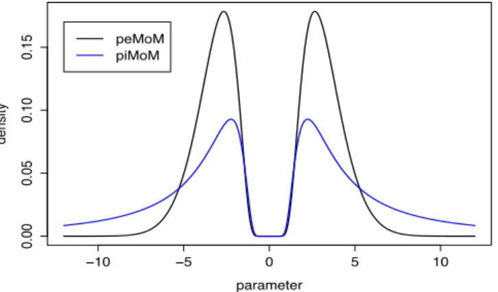
−10 −5 0 5 10 0.00 0.05 0.10 0.15 parameter density peMoM piMoM

Figure 2.1: Nonlocal prior density functions for a single regression coefficient with⌧ = 5; for

the piMoM prior,r= 1.

The normalizing constantCcan be explicitly calculated as

C =

Z ₁

1

exp_{ t2/(2 2⌧) ⌧/t2_}dt = (2⇡ 2⌧)1/2exp_{ (2/ 2)1/2_}, (2.3)

sinceR exp{ µ/t2 _⇣_t2_}_dt _{= (}_⇡_/_⇣₎1/2_exp_{ _2(µ_⇣₎1/2_}_.

Second, for a fixed positive integerr, the product inverse-moment (piMoM) prior density (Johnson and Rossell, 2012) for kis given by

⇡( k| 2,⌧,k) =C⇤ |k| |k| Y

j=1

[( k,j) 2rexp{ ⌧/ k2,j}], (2.4)

whereC⇤ =⌧ r+1/2 _(r _1/2)_for_{r >}_1/2_and ₍_·₎_{is the gamma function.}

The piMoM and peMoM prior densities are nonlocal in the sense that the density value at the origin is exactly zero. This feature of the densities for a single regression coefficient is illustrated in Figure 2.1. Since the piMoM prior densities and the peMoM prior densities have the same termexp_{ ⌧/ 2_}_{that controls the behavior of the density function around the}

(36)

similar properties. Further details regarding this point are discussed in Section 2.4.

I focus on these two classes of nonlocal priors in the sequel. Note that in both (2.2) and (2.4),⇡( k) = 0when k = 0; a defining feature of nonlocal priors. The distinction between

the peMoM and the piMoM priors mainly involves their tail behavior. Whereas peMoM priors possess Gaussian tails, the piMoM prior densities have inverse polynomial tails. For example, piMoM densities with r = 1 have Cauchy-like tails, which has implications for their finite sample consistency and asymptotic bias in posterior mean estimates of regression coefficients. Because similar constraints are imposed on the hyperparameter⌧ appearing in both (2.2) and

(2.4), at the risk of some ambiguity I use the same symbol for the two hyperparameters in these equations.

In addition to imposing priors on the regression parameters given a model, I need to place a prior on the space of models to complete the prior specification. I consider a uniform prior on the model space restricted to models having size less than or equal toqn, withqn< n, i.e.,

⇡(k)_/I(_|k_|_qn), (2.5)

whereI(·)denotes the indicator function and with a slight abuse of notation, I denote the prior on the space of models by⇡ as well. Similar priors have been considered in the literature by

Jiang (2007) and Liang et al. (2013). Since the peMoM and piMoM priors already induce a strong penalty on the size of the model space (see Section 2.4), I do not need to additionally penalize larger models using, for example, model space priors of the type discussed in Scott and Berger (2010).

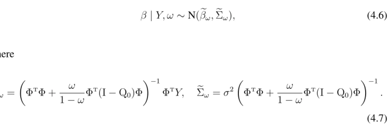
Under a peMoM prior (2.2) on the regression coefficients, the marginal likelihoodmk(y)

under modelkgiven 2 _{can be obtained by integrating out}

k, resulting in

mk(y) = (2⇡ 2) n

(37)

where e Rk = yT(In Pek)y, Pek =Xk(XkTXk+ 1/⌧Ik) 1XkT, Qk = Z exp_{ ( k ek)T⌃e_k1( k ek)/(2 2) |k| X j=1 ⌧/ _k2_,j_}d k, (2.6) e_k _{= (X}T kXk+ 1/⌧Ik) 1XkTy, ⌃ek= (XkTXk+ 1/⌧Ik) 1.

Similarly, the marginal likelihood using the piMoM prior densities (2.4) can be expressed asmk(y) = (2⇡ 2) n 2 C⇤ |k|Q⇤ k exp{ R⇤k/(2 2)}, where R⇤k = yT(In Pk)y, Pk =Xk(XkTXk) 1XkT, Q⇤k = Z _Y|k| j=1 2r k,j exp{ ( k bk)T⌃⇤k 1( k bk)/(2 2) |k| X j=1 ⌧/ k2,j}d k, (2.7) b_k = (XT kXk) 1XkTy, ⌃⇤k = (X T kXk) 1.

The integrals forQkandQ⇤kcannot be obtained in closed form, so for computational purposes

I make Laplace approximations tomk(y). The expressions for the marginal likelihood derived

here is nevertheless important for theoretical studies in Section 2.4. 2.3 Numerical Results

2.3.1 Simulation Studies Using Precision-Recall Curves

To illustrate the performance of nonlocal priors in ultrahigh-dimensional settings and to compare their performance with other methods, I calculated precision-recall curves Davis and Goadrich (2006) for all selection procedures. A precision-recall curve plots the precision = TP/(TP + FP) versus recall (or sensitivity) = TP/(TP + FN), where TP, FP and FN respectively denote the number of true positives, false positives, and false negatives, as the tuning parameter is varied. The efficacy of a procedure can be measured by the area under the precision-recall

(38)

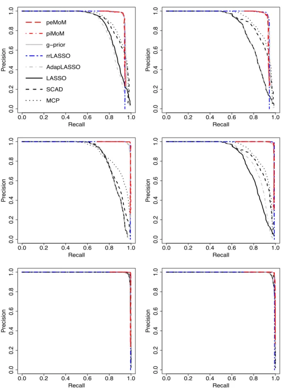
curve; the greater the area, the more accurate the method. Since both precision and recall take values in [0,1], the area under the curve for an ideal precision-recall curve is 1. I used two (n, p)combinations, namely(n, p) = (400,10000)and(n, p) = (400,20000), and plotted the average of the precision-recall curves obtained from100 independent replicates of each pro-cedure. To evaluate the marginal likelihood of each model, I used the Laplace approximation method.

I compared the performance of peMoM and piMoM priors to a number of frequentist penal-ized likelihood methods: Lasso (Tibshirani, 1996), adaptive Lasso (Zou, 2006), Scad (Fan and Li, 2001), and Minimax Concave Penalty (MCP) (Zhang, 2010). I used theRpackagencvreg

to fit these penalized likelihood methods. I also included the reciprocal Lasso in the simulation studies. However, due to computational constraints involved in implementing the full rLasso procedure, I followed the recommendation in Song and Liang (2015) and instead implemented the reduced rLasso. The reduced rLasso procedure is a simplified version of rLasso that uses the least square estimators of when minimizing the rLasso objective function.

I considered Zellner’sg-prior Zellner (1986); Liang et al. (2008) as a competing Bayesian method, with k | k, 2 ⇠ N(0, g 2(XkTXk) 1) and g a tuning parameter. With the prior ⇡( 2₎ _/ _1/ 2_{, the marginal likelihood}_m

k(y) / (1 +g) |k|/2{1 +g(1 Dk2)} (n 1)/2 can

be obtained in a closed form; see for example, (Liang et al., 2008, pp 412), where D2 k is the

ordinary coefficient of determination for the modelk.

A uniform model prior (2.5) was considered for all Bayesian procedures. This prior was chosen for several reasons. First, construction of the PR curves requires maximization over model hyperparameters, which is most easily achieved if there is only one unknown hyperpa-rameter. I also wished to avoid providing an advantage to the Bayesian methods by introducing additional tuning parameters into these methods that were not present in the penalized likeli-hood methods. Furthermore, the use of non-uniform priors on the model space introduces (at least) one more degree of freedom into the comparisons between methods, and my intent was

(39)

to compare the effects of the penalties imposed on regression coefficients by both penalized likelihood and Bayesian methods. At first blush, this might appear to put Bayesian methods like those based on the g-prior at a disadvantage, since such methods do not yield consistent variable selection even inp < nsettings without prior sparsity penalties on the model space (whengis held fixed asnincreases). However, in the construction of PR curves, I allowed prior hyperparameters to increase withn, which effectively allowed the Bayesian methods to impose additional sparseness penalties through the introduction of large hyperparameter values.

I arbitrarily fixedr = 1for the piMoM prior (2.4) and used an inverse-gamma prior on 2 with parameters(0.1,0.1)for the peMoM, piMoM priors, andg-priors. Posterior computations for the peMoM, piMoM andg-priors were implemented using the Simplified Shotgun Stochas-tic Search with Screening (S5) algorithm described in Chapter 3. The maximum a posteriori model was used in each case to summarize the model selection performance. The precision-recall curves are drawn by varying the hyperparameters (⌧ for the nonlocal priors andgfor the g-priors) so the comparison between the model selection based on the nonlocal priors and the g-prior is free of the choice of hyperparameters. Because of their high computational burden, I could not include BASAD Narisetty and He (2014) in the comparisons.

For each simulation setting, I simulated data according to a Gaussian linear model as in (2.1) with the fixed true model t = _{1,2,3,4,5_} with the true regression coefficient 0

t =

(0.50,0.75,1.00,1.25,1.50)T and = 1.5. Also, the signs of the true regression coefficients

were randomly determined with probability one-half. Each row ofX was independently gen-erated from aN(0,⌃)distribution with one of the following covariance structures:

Case (1): compound symmetry design;⌃jj0 = 0.5, ifj 6=j0 and⌃_jj = 1,1j, j0 p.

Case (2): autoregressive correlated design;⌃jj0 = 0.5|j j0|,1j, j0 p.

Case (3): isotropic design;⌃= Ip.

(40)

different methods across the two (n,p) pairs and the three covariate designs. From Figure 2.2, it is evident that the precision-recall curves for the peMoM and piMoM priors have an overall better performance than the penalized likelihood methods Lasso, adaptive Lasso, Scad, and MCP. For decision procedures having the same power, this implies that the nonlocal priors achieve lower false discovery rates. As discussed in Section 2.5, since the reduced rLasso shares the same nonlocal kernel as the nonlocal priors, it has a similar selection performance. The figure also shows that Zellner’sg-prior attains comparable performance with the nonlocal priors in terms of the precision-recall curves.

2.3.2 Further Comparison with Zellner’sg-prior

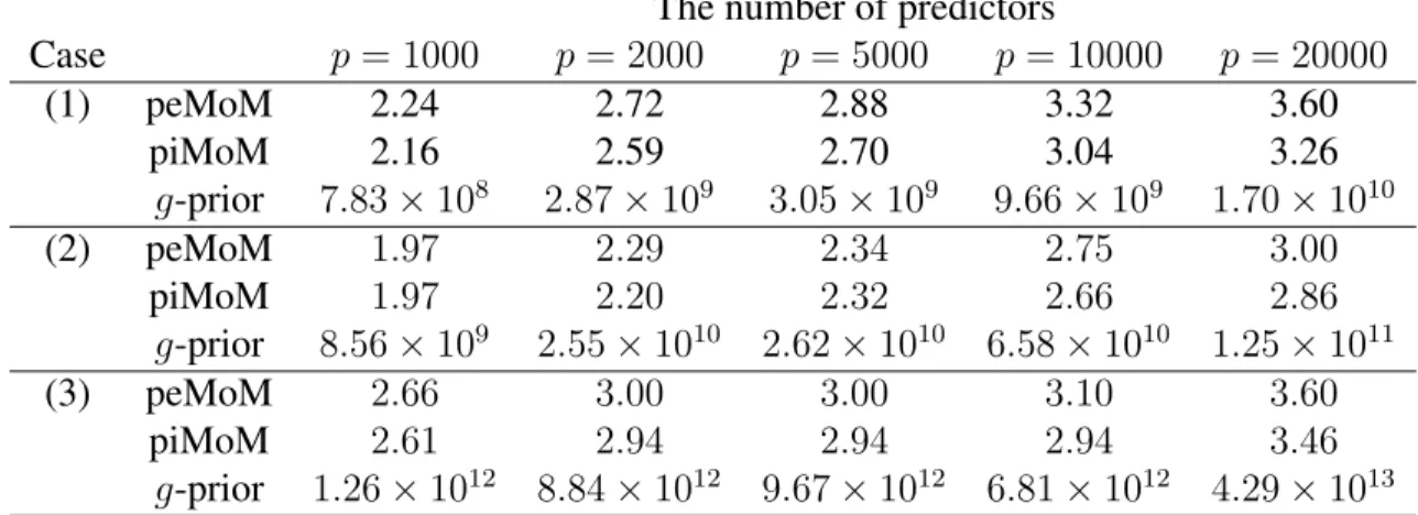
The similarity of the performances of theg-prior and the nonlocal priors in terms of precision-recall curves begs for closer comparisons of these procedures. For this reason, I also investi-gated the concentration of the posterior densities around their maximum models. To this end, I fixedp = 20,000and variedn from150to400; the data generating mechanism was exactly the same as in Section 2.3.1. The left column of Figure 2.3 displays the posterior probability of the true model under the peMoM, piMoM andg-prior models versusn for the three covari-ate designs in Section 2.3.1. The plot shows that the posterior probability of the true model increases withn for all three methods, with the peMoM and piMoM priors almost uniformly dominating theg-prior, implying a higher concentration of the posterior around the true model for the nonlocal priors.

This tendency is confirmed in the right panel of Figure 2.3, where I plot the number of models k which achieve a posterior odds ratio ⇡(k _| y)/⇡(bk _| y) > 0.001, where kb is the

maximum a posteriori model. This plot clearly shows that the posterior distribution on the model space from the g-priors is more diffuse than those obtained using the nonlocal prior methods. These comparisons were based on fitting the hyperparametersg and⌧ at their oracle

(41)

0.0 0.2 0.4 0.6 0.8 1.0 0.0 0.2 0.4 0.6 0.8 1.0 Recall Precision peMoM piMoM g−prior rrLASSO AdapLASSO LASSO SCAD MCP 0.0 0.2 0.4 0.6 0.8 1.0 0.0 0.2 0.4 0.6 0.8 1.0 Recall Precision 0.0 0.2 0.4 0.6 0.8 1.0 0.0 0.2 0.4 0.6 0.8 1.0 Recall Precision 0.0 0.2 0.4 0.6 0.8 1.0 0.0 0.2 0.4 0.6 0.8 1.0 Recall Precision 0.0 0.2 0.4 0.6 0.8 1.0 0.0 0.2 0.4 0.6 0.8 1.0 Recall Precision 0.0 0.2 0.4 0.6 0.8 1.0 0.0 0.2 0.4 0.6 0.8 1.0 Recall Precision

Figure 2.2: Plot of the mean precision-precision curves over 100 datasets with (n, p) = (400,10000)(first column) and (n, p) = (400,20000)(second column). Top: case (1); mid-dle: case (2); bottom: case (3).

(42)

n poster ior probability 150 200 250 300 400 0.0 0.2 0.4 0.6 0.8 1.0 peMoM piMoM g−prior n # of models 150 200 250 300 400 0 20 40 60 80 100 n poster ior probability 150 200 250 300 400 0.0 0.2 0.4 0.6 0.8 1.0 n # of models 150 200 250 300 400 0 20 40 60 80 100 n poster ior probability 150 200 250 300 400 0.0 0.2 0.4 0.6 0.8 1.0 n # of models 150 200 250 300 400 0 20 40 60 80 100

Figure 2.3: Averaged posterior true model probability and the number of models which attain the posterior odds ratio, with respect to the maximum a posteriori model, larger than 0.001 with the fixedp= 20000and varyingn. Top: case (1); middle: case (2); bottom: case (3).

(43)

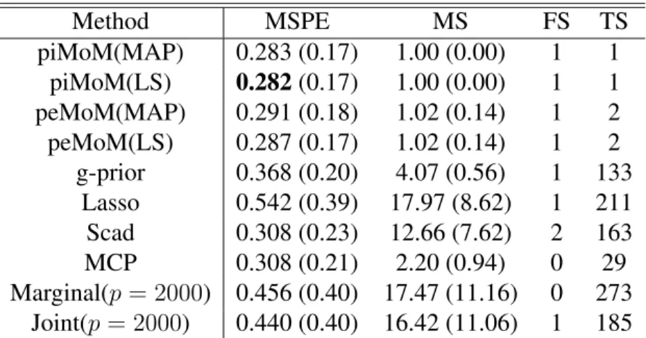
Table 2.1: Optimal hyperparameters for Bayesian model selection methods The number of predictors

Case p= 1000 p= 2000 p= 5000 p= 10000 p= 20000 (1) peMoM 2.24 2.72 2.88 3.32 3.60 piMoM 2.16 2.59 2.70 3.04 3.26 g-prior 7.83_⇥108 _2.87_⇥₁₀9 _3.05_⇥₁₀9 _9.66_⇥₁₀9 _1.70_⇥₁₀10 (2) peMoM 1.97 2.29 2.34 2.75 3.00 piMoM 1.97 2.20 2.32 2.66 2.86 g-prior 8.56⇥109 _2.55_⇥₁₀10 _2.62_⇥₁₀10 _6.58_⇥₁₀10 _1.25_⇥₁₀11 (3) peMoM 2.66 3.00 3.00 3.10 3.60 piMoM 2.61 2.94 2.94 2.94 3.46 g-prior 1.26_⇥1012 _8.84_⇥₁₀12 _9.67_⇥₁₀12 _6.81_⇥₁₀12 _4.29_⇥₁₀13 value ofn.

The magnitudes of the oracle hyperparameters under each model also present an interesting contrast between the local and nonlocal priors. I observed that the oracle value ofg increased rapidly withp, whereas the oracle value of⌧ was much more stable. This phenomenon is

illus-trated in Table 2.1, which shows the oracle hyperparameter value averaged over 100 replicates for the three different covariate designs in Section 2.3.1. For this comparison, I fixedn = 400 and varied p between1000 and 20,000; five representative values are displayed. The oracle values for g are on a completely different scale from the oracle values of ⌧, and they vary

more with p. This table confirms the recommendations in George and Foster (2000) for set-tingg =p2 _{based on minimax arguments. However, the finite sample behavior of the optimal}

choice ofgis unclear, which means that the large variance of the optimal hyperparameter value is likely to hinder the selection ofg in real applications. Finally, I note that such large values ofg effectively convert the localg-priors into nonlocal priors by collapsing theg-prior density to 0 at the origin.

(44)

2.4 Model Selection Consistency

The empirical performance of the peMoM and piMoM priors suggests that the hyperpa-rameter⌧ should be increased slowly withp. While Johnson and Rossell (2012) were able to

show strong selection consistency with a fixed value of⌧, it is not clear whether their proof can

be extended top ncases. Motivated by the empirical findings of the last section, I next in-vestigated the strong consistency properties of peMoM and piMoM priors when⌧ was allowed

to grow at a logarithmic rate inp. I found that in such cases, both peMoM and piMoM priors achieve model selection consistency under standard regularity assumptions when pincreases sub-exponentially withn, i.e.,logp=O(n↵₎_for_↵ ₂_(0,_1).

Henceforth, I use⌧n,pinstead of⌧ to denote the hyperparameter in the peMoM and piMoM priors in (2.2) and (2.4) respectively. The normalizing constants for these priors are now de-noted by Cn,p and C_n,p⇤ , respectively. Before providing my theoretical results, I first state a number of regularity conditions. Let ⌫j(A) denote thej-th largest nonzero eigenvalue of an arbitrary matrixA, and let

⌫k_⇤ = min 1jmin(n,|k|)⌫j(X T kXk/n), ⌫k⇤ = max 1jmin(n,|k|)⌫j(X T kXk/n). (2.8)

For sequencesanandbn,an⌫bnindicatesbn=O(an), andan bnindicatesbn=o(an). With this notation, I assume that the following regularity conditions apply.

Assumption 1. There exists↵₂(0,1)such thatlogp=O(n↵_). Assumption 2. logp ⌧n,p n. Assumption 3. |k|qn, whereqn ⌧n,p logp. Assumption 4. min k:|k|qn ⌫k_⇤ ⌧n,p n .

(45)

Assumption 5. C1 <⌫t⇤ ⌫t⇤ < C2 for some positive constantsC1 andC2.

Several comments regarding these conditions are worth making. Assumption 1 allows p to grow sub-exponentially with n. My theoretical results continue to hold when p grows polynomially inn, i.e., at the rateO(n )for some >1. Assumption 2 reflects the empirical findings about the oracle ⌧ ⌘ ⌧n,p in Section 2.3.1, which was observed to grow slowly with p. I need the bound on qn in Assumption 3 to ensure that the least square estimator of a model is consistent when a model contains the true model. In thep n setting, Johnson and Rossell (2012) assumed that all eigenvalues of the Gram matrix(XT

kXk)/nare bounded above

and below by global constants for all k. However, this assumption is no longer viable when

p n and I replace that by Assumption 4, where the minimum of the minimum eigenvalue of (XT

kXk)/n over all submodels kwith |k|  qn is allowed to decrea