An Optimal Real-Time Scheduling Algorithm for Multiprocessors
Hyeonjoong Cho
ETRI
Daejeon, 305-714, Korea
[email protected]
Binoy Ravindran
ECE Dept., Virginia Tech
Blacksburg, VA 24061, USA
[email protected]
E. Douglas Jensen
The MITRE Corporation
Bedford, MA 01730, USA
[email protected]
Abstract
We present an optimal real-time scheduling algorithm for multiprocessors — one that satisfies all task deadlines, when the total utilization demand does not exceed the uti-lization capacity of the processors. The algorithm called LLREF, is designed based on a novel abstraction for rea-soning about task execution behavior on multiprocessors: the Time and Local Execution Time Domain Plane (or T-L plane). T-LT-LREF is based on the fluid scheduling model and the fairness notion, and uses the T-L plane to describe fluid schedules without using time quanta, unlike the opti-mal Pfair algorithm (which uses time quanta). We show that scheduling for multiprocessors can be viewed as repeatedly occurring T-L planes, and feasibly scheduling on a single T-L plane results in the optimal schedule. We analytically establish the optimality of LLREF. Further, we establish that the algorithm has bounded overhead, and this bound is in-dependent of time quanta (unlike Pfair). Our simulation results validate our analysis on the algorithm overhead.
1
Introduction
Multiprocessor architectures (e.g., Symmetric Multi-Processors or SMPs, Single Chip Heterogeneous Multipro-cessors or SCHMs) are becoming more attractive for em-bedded systems, primarily because major processor manu-facturers (Intel, AMD) are making them decreasingly ex-pensive. This makes such architectures very desirable for embedded system applications with high computational workloads, where additional, cost-effective processing ca-pacity is often needed. Responding to this trend, RTOS vendors are increasingly providing multiprocessor platform support — e.g., QNX Neutrino is now available for a vari-ety of SMP chips [12]. But this exposes the critical need for real-time scheduling for multiprocessors — a compara-tively undeveloped area of real-time scheduling which has recently received significant research attention, but is not yet well supported by the RTOS products. Consequently,
the impact of cost-effective multiprocessor platforms for embedded systems remains nascent.
One unique aspect of multiprocessor real-time schedul-ing is the degree of run-time migration that is allowed for job instances of a task across processors (at scheduling events). Example migration models include: (1)full migra-tion, where jobs are allowed to arbitrarily migrate across processors during their execution. This usually implies a global scheduling strategy, where a single shared schedul-ing queue is maintained for all processors and a processor-wide scheduling decision is made by a single (global) scheduling algorithm; (2) no migration, where tasks are statically (off-line) partitioned and allocated to processors. At run-time, job instances of tasks are scheduled on their respective processors by processors’ local scheduling algo-rithm, like single processor scheduling; and (3) restricted migration, where some form of migration is allowed—e.g., at job boundaries.
The partitioned scheduling paradigm has several advan-tages over the global approach. First, once tasks are allo-cated to processors, the multiprocessor real-time schedul-ing problem becomes a set of sschedul-ingle processor real-time scheduling problems, one for each processor, which has been well-studied and for which optimal algorithms exist. Second, not migrating tasks at time means reduced run-time overhead as opposed to migrating tasks that may suffer cache misses on the newly assigned processor. If the task set is fixed and known a-priori, the partitioned approach pro-vides appropriate solutions [3].
The global scheduling paradigm also has advantages, over the partitioned approach. First, if tasks can join and leave the system at run-time, then it may be necessary to re-allocate tasks to processors in the partitioned approach [3]. Second, the partitioned approach cannot produce optimal real-time schedules — one that meets all task deadlines when task utilization demand does not exceed the total pro-cessor capacity — for periodic task sets [14], since the par-titioning problem is analogous to the bin-packing problem which is known to be NP-hard in the strong sense. Third, in some embedded processor architectures with no cache and
simpler structures, the overhead of migration has a lower impact on the performance [3]. Finally, global scheduling can theoretically contribute to an increased understanding of the properties and behaviors of retime scheduling al-gorithms for multiprocessors. See [10] for a detailed dis-cussion on this.
Carpenteret al.[4] have catalogued multiprocessor real-time scheduling algorithms considering the degree of job migration and the complexity of priority mechanisms em-ployed. (The latter includes classes such as (1)static, where task priorities never change, e.g., rate-monotonic (RM); (2) dynamic but fixed within a job, where job priorities are fixed, e.g., earliest-deadline-first (EDF); and (3) fully-dynamic, where job priorities are dynamic. )
The Pfair class of algorithms [2] that allow full migration and fully dynamic priorities have been shown to be theo-retically optimal—i.e., they achieve a schedulable utiliza-tion bound (below which all tasks meet their deadlines) that equals the total capacity of all processors. However, Pfair algorithms incur significant run-time overhead due to their quantum-based scheduling approach [7, 14]: under Pfair, tasks can be decomposed into several small uniform seg-ments, which are then scheduled, causing frequent schedul-ing and migration.
(a)
(b)
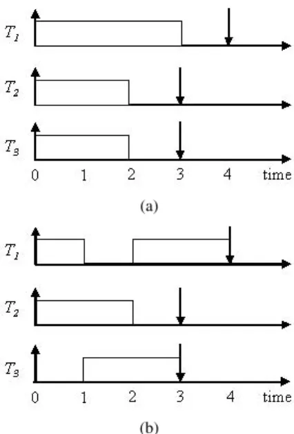
Figure 1:A Task Set that EDF Cannot Schedule On Two Processors
Thus, scheduling algorithms other than Pfair—e.g., global EDF [7–9, 13], have also been intensively studied though their schedulable utilization bounds are lower. Fig-ure 1(a) shows an example task set that global EDF cannot feasibly schedule. Here, taskT1will miss its deadline when the system is given two processors. However, there exists a schedule that meets all task deadlines; this is shown in Figure 1(b).
Interestingly, we observe in Figure 1(b) that the schedul-ing event at time 1, where taskT1is split to make all tasks schedulable is not a traditional scheduling event (such as a task release or a task completion). This simple obser-vation implies that we may need more scheduling events to split tasks to construct optimal schedules, such as what Pfair’s quantum-based approach does. However, it also raises another fundamental question: is it possible to split tasks to construct optimal schedules, not at time quantum expiration, but perhaps at other scheduling events, and con-sequently avoid Pfair’s frequent scheduling and migration overheads? If so, what are those scheduling events?
In this paper, we answer these questions.1 We present an optimal real-time scheduling algorithm for multiprocessors, which is not based on time quanta. The algorithm called LLREF, is based on the fluid scheduling model and the fair-ness notion. We introduce a novel abstraction for reasoning about task execution behavior on multiprocessors, called the
time and local remaining execution-time plane(abbreviated as theT-L plane). T-L plane makes it possible for us to en-vision that the entire scheduling over time is just the repeti-tion of T-L planes in various sizes, so that feasible schedul-ing in a sschedul-ingle T-L plane implies feasible schedulschedul-ing over all times. We define two additional scheduling events and show when they should happen to maintain the fairness of an optimal schedule, and consequently establish LLREF’s scheduling optimality. We also show that the overhead of LLREF is tightly bounded, and that bound depends only upon task parameters. Furthermore, our simulation experi-ments on algorithm overhead validate our analysis.
The rest of the paper is organized as follows: In Sec-tion 2, we discuss the raSec-tionale behind T-L plane and present the scheduling algorithm. In Section 3, we prove the opti-mality of our algorithm, establish the algorithm overhead bound, and report simulation studies. The paper concludes in Section 4.
2
LLREF Scheduling Algorithm
2.1
Model
We consider global scheduling, where task migration is not restricted, on an SMP system withM identical proces-sors. We consider the application to consist of a set of tasks, denotedT={T1,T2, ...,TN}. Tasks are assumed to arrive periodically at their release timesri. Each taskTihas an ex-ecution timeci, and a relative deadlinediwhich is the same as its periodpi. The utilizationuiof a taskTiis defined as
ci/diand is assumed to be less than 1. Similar to [1, 7], we assume that tasks may be preempted at any time, and are 1There exists a variant of EDF, calledEarliest Deadline until Zero
Lax-ity(EDZL), which allows another scheduling event to split tasks, but it does not offer the optimality for multiprocessors [11].
independent, i.e., they do not share resources or have any precedences.
We consider a non-work conserving scheduling policy; thus processors may be idle even when tasks are present in the ready queue. The cost of context switches and task migrations are assumed to be negligible, as in [1, 7].
2.2
Time and Local Execution Time Plane
In thefluid scheduling model, each task executes at a constant rate at all times [10]. The quantum-based Pfair scheduling algorithm, the only known optimal algorithm for the problem that we consider here, is based on the fluid scheduling model, as the algorithm constantly tracks the allocated task execution rate through task utilization. The Pfair algorithm’s success in constructing optimal multipro-cessor schedules can be attributed tofairness— informally, all tasks receive a share of the processor time, and thus are able to simultaneously make progress. P-fairness is a strong notion of fairness, which ensures that at any instant, no ap-plication is one or more quanta away from its due share (or fluid schedule) [2, 5]. The significance of the fairness con-cept on Pfair’s optimality is also supported by the fact that taskurgency, as represented by the task deadline is not suf-ficient for constructing optimal schedules, as we observe from the poor performance of global EDF for multiproces-sors.
Figure 2:Fluid Schedule versus a Practical Schedule
Toward designing an optimal scheduling algorithm, we thus consider the fluid scheduling model and the fairness notion. To avoid Pfair’s quantum-based approach, we con-sider an abstraction called the Time and Local Execution Time Domain Plane (or abbreviated as the T-L plane), where tokens representing tasks move over time. The T-L plane is inspired by the T-L-C plane abstraction introduced by Dertouzoset al.in [6]. We use the T-L plane to describe fluid schedules, and present a new scheduling algorithm that
is able to track the fluid schedule without using time quanta. Figure 2 illustrates the fundamental idea behind the T-L plane. For a task Ti withri, ci anddi, the figure shows a 2-dimensional plane with time represented on the x-axis and the task’s remaining execution time represented on the y-axis. Ifri is assumed as the origin, the dotted line from
(0, ci) to(di,0) indicates the fluid schedule, the slope of which is −ui. Since the fluid schedule is ideal but prac-tically impossible, the fairness of a scheduling algorithm depends on how much the algorithm approximates the fluid schedule path.
WhenTi runs like in Figure 2, for example, its execu-tion can be represented as a broken line between (0, ci)
and (di,0). Note that task execution is represented as a line whose slope is -1 since x and y axes are in the same scale, and the non-execution over time is represented as a line whose slope is zero. It is clear that the Pfair algorithm can also be represented in the T-L plane as a broken line based on time quanta.
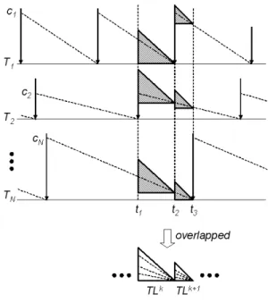
Figure 3:T-L Planes
When N number of tasks are considered, their fluid schedules can be constructed as shown in Figure 3, and a right isosceles triangle for each task is found between ev-ery two consecutive scheduling events2andNtriangles be-tween every two consecutive scheduling events can be over-lapped together. We call this as the T-L planeT Lk, wherek
is simply increasing over time. The size ofT Lkmay change overk. The bottom side of the triangle represents time. The left vertical side of the triangle represents the axis of a part 2In this paper, we assume that all tasks have their deadlines equal to
their period parameters. Thus, two consecutive scheduling events are task releases.
of tasks’ remaining execution time, which we call thelocal remaining execution time,li, which is supposed to be con-sumed before eachT Lkends. Fluid schedules for each task can be constructed as overlapped in eachT Lkplane, while keeping their slopes.
2.3
Scheduling in T-L planes
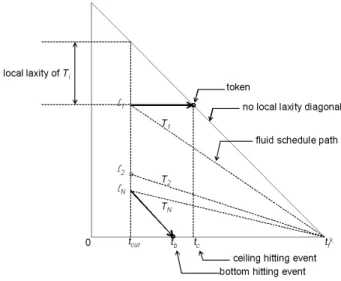
The abstraction of T-L planes is significantly meaning-ful in scheduling for multiprocessors, because T-L planes are repeated over time, and a good scheduling algorithm for a single T-L plane is able to schedule tasks for all repeated T-L planes. Here, good scheduling means being able to con-struct a schedule that allows all tasks’ execution in the T-L plane to approximate the fluid schedule as much as possible. Figure 4 details thekthT-L plane.
Figure 4:kthT-L Plane
The status of each task is represented as atokenin the T-L plane. The token’s location describes the current time as a value on the horizontal axis and the task’s remaining ex-ecution time as a value on the vertical axis. The remaining execution time of a task here means one that must be con-sumed until the timetkf, and not the task’s deadline. Hence, we call it,localremaining execution time.
As scheduling decisions are made over time, each task’s token moves in the T-L plane. Although ideal paths of to-kens exist as dotted lines in Figure 4, the toto-kens are only allowed to move in two directions. (Therefore, tokens can deviate from the ideal paths.) When the task is selected and executed, the token moves diagonally down, asTN moves. Otherwise, it moves horizontally, asT1 moves. IfM pro-cessors are considered, at mostM tokens can diagonally move together. The scheduling objective in the kth T-L plane is to make all tokens arrive at the rightmost vertex of the T-L plane—i.e.,tkf with zero local remaining
execu-tion time. We call this successful arrival,locally feasible. If all tokens are made locally feasible at each T-L plane, they are possible to be scheduled throughout every consecutive T-L planes over time, approximating all tasks’ ideal paths.
For convenience, we define thelocal laxityof a taskTi astkf−tcur−li, wheretcuris the current time. The oblique side of the T-L plane has an important meaning: when a token hits that side, it implies that the task does not have any local laxity. Thus, if it is not selected immediately, then it cannot satisfy the scheduling objective of local feasibil-ity. We call the oblique side of the T-L planeno local laxity diagonal(or NLLD). All tokens are supposed to stay in be-tween the horizontal line and the local laxity diagonal.
We observe that there are two time instants when the scheduling decision has to be made again in the T-L plane. One instant is when the local remaining execution time of a task is completely consumed, and it would be better for the system to run another task instead. When this occurs, the token hits the horizontal line, asTN does in Figure 4. We call it thebottom hitting event (or event B). The other in-stant is when the local laxity of a task becomes zero so that the task must be selected immediately. When this occurs, the token hits the NLLD, asT1 does in Figure 4. We call it theceiling hitting event(or event C). To distinguish these events from traditional scheduling events, we call events B and Csecondary events.
To provide local feasibility, M of the largest local re-maining execution timetasks are selected first (or LLREF) for every secondary event. We call this, the LLREF schedul-ing policy. Note that the task havschedul-ing zero local remain-ing execution time (the token lyremain-ing on the bottom line in the T-L plane) is not allowed to be selected, which makes our scheduling policy non work-conserving. The tokens for these tasks are calledinactive, and the others with more than zero local remaining execution time are called active. At timetkf, the time instant for the event of the next task re-lease, the next T-L planeT Lk+1starts and LLREF remains valid. Thus, the LLREF scheduling policy is consistently applied for every event.
Algorithm 1: LLREF
Input :T={T1,...,TN},ζr: Ready queue, M:# of processors 1
Output : array of dispatched tasks to processors 2 sortByLLRET(ζr); 3 {T1, ..., TM}=selectTasks(ζr); 4 return{T1, ..., TM}; 5
LLREF is briefly described in Algorithm 1, whereζis a queue of active tokens. It is invoked at every event including secondary event B and C. We assume that each task’sliis updated before the algorithm starts. When it is invoked,
sortByLLREFsorts tokens in the order of largest local remaining execution time and selectTasksselectsM
active tasks to dispatch to processors. The computational complexity of this algorithm isO(nlogn)due to the sorting process but it can be reduced (or fastened), which will be discussed in Section 4.
3
Algorithm Properties
A fundamental property of the LLREF scheduling algo-rithm is its scheduling optimality—i.e., the algoalgo-rithm can meet all task deadlines when the total utilization demand does not exceed the capacity of the processors in the sys-tem. In this section, we establish this by proving that LL-REF guarantees local feasibility in the T-L plane.
3.1
Critical Moment
Figure 5 shows an example of token flow in the T-L plane. All tokens flow from left to right over time. LL-REF selectsM tokens fromN active tokens and they flow diagonally down. The others which are not selected, on the other hand, take horizontal paths. When the event C or B happens, denoted bytj where 0 < j < f, LLREF is in-voked to make a scheduling decision.
Figure 5:Example of Token Flow
We define thelocal utilizationri,jfor a taskTiat timetj
to be tli,j
f−tj, which describes how much processor capacity
needs to be utilized for executingTiwithin the remaining time untiltf. Here, li,j is the local remaining execution time of taskTiat timetj. Whenkis omitted, it implicitly means the currentkthT-L plane.
Theorem 1(Initial Local Utilization Value in T-L plane). Let all tokens arrive at the rightmost vertex in the(k−1)th
T-L plane. Then, the initial local utilization valueri,0=ui
for all taskTiin thekthT-L plane.
Proof. If all tokens arrive attkf−1withli= 0, then they can restart in the next T-L plane (thekthT-L plane) from the positions where their ideal fluid schedule lines start. The
slope of the fluid schedule path of taskTiisui. Thus,ri,0= li,0/tf =ui.
Well-controlled tokens, both departing and arriving points of which are the same as those of their fluid schedule lines in the T-L plane (even though their actual paths in the T-L plane are different from their fluid schedule paths), im-ply that all tokens are locally feasible. Note that we assume
ui≤1andui≤M.
Figure 6:Critical Moment
We definecritical momentto describe the sufficient and necessary condition that tokens are not locally feasible. (Local infeasibility of the tokens implies that all tokens do not simultaneously arrive at the rightmost vertex of the T-L plane.) Critical moment is the first secondary event time when more than M tokens simultaneously hit the NLLD. Figure 6 shows this. Right after the critical moment, only
M tokens from those on the NLLD are selected. The non-selected ones move out of the triangle, and as a result, they will not arrive at the right vertex of the T-L plane. Note that only horizontal and diagonal moves are permitted for tokens in the T-L plane.
Theorem 2(Critical Moment). At least one critical moment occurs if and only if tokens are not locally feasible in the T-L plane.
Proof. We prove both the necessary and sufficient condi-tions.
Case 1. Assume that a critical moment occurs. Then, non-selected tokens move out of the T-L plane. Since only -1 and 0 are allowed for the slope of the token paths, it is impossible that the tokens out of the T-L plane reach the rightmost vertex of the T-L plane.
Case 2. We assume that when tokens are not locally feasible, no critical moment occurs. If there is no critical moment, then the number of tokens on the NLLD never ex-ceedsM. Thus, all tokens on the diagonal can be selected by LLREF up to timetf. This contradicts our assumption that tokens are not locally feasible.
We define total local utilization at the jth secondary event,Sj, asNi ri,j.
Corollary 3(Total Local Utilization at Critical Moment). At the critical moment which is the jth secondary event,
Sj > M.
Proof. The local remaining execution timeli,jfor the tasks on the NLLD at the critical moment of thejth secondary event is tf −tj, because the T-L plane is an isosceles triangle. Therefore, Sj = Ni=1ri,j = Mi=1ttf−tj
f−tj +
N
i=M+1tfl−itj =M +
N
i=M+1tfl−itj > M.
From the task perspective, the critical moment is the time when more thanM tasks have no local laxity. Thus, the scheduler cannot make them locally feasible withM pro-cessors.
3.2
Event C
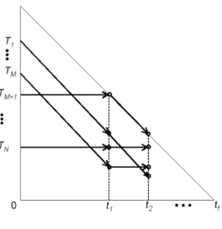
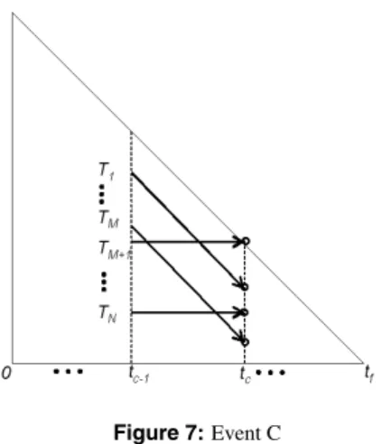
Event C happens when a non-selected token hits the NLLD. Note that selected tokens never hit the NLLD. Event C indicates that the task has no local laxity and hence, should be selected immediately. Figure 7 illustrates this, where event C happens at time tc when the token TM+1
hits the NLLD.
Note that this is under the basic assumption that there are more thanM tasks, i.e.,N > M. This implicit assumption holds in Section 3.2 and 3.3. We will later show the case whenN ≤M.
For convenience, we give lower indexito the token with higher local utilization, i.e.,ri,j≥ri+1,jwhere1≤i < N
and∀j, as shown Figure 7. Thus, LLREF select tasks from
T1toTM and their tokens move diagonally.
Figure 7:Event C
Lemma 4 (Sufficient and Necessary Condition for Event C). When1−rM+1,c−1 ≤rM,c−1, the event C occurs at timetc, whereri,c−1≥ri+1,c−1,1≤i < N.
Proof. If the secondary event at timetc is event C, then token TM+1 must hit the NLLD earlier than when token
TM hit the bottom of the T-L plane. The time whenTM+1 hits the NLLD istc−1+ (tf−tc−1−lM+1,c−1). On the contrary, the time when the tokenTM hits the bottom of the T-L plane istc−1+lM,c−1. tc−1+ (tf−tc−1−lM+1,c−1)< tc−1+lM,c−1 1− lM+1,c−1 tf −tc−1 < lM,c−1 tf−tc−1. Thus,1−rM+1≤rM attc−1.
Corollary 5(Necessary Condition for Event C). Event C occurs at timetconly ifSc−1> M(1−rM+1,c−1), where
ri,c−1≥ri+1,c−1,1≤i < N. Proof. Sc−1= M i=1 ri,c−1+ N i=M+1 ri,c−1> M i=1 ri,c−1≥M·rM,c−1. Based on Lemma 4,M·rM,c−1≥M·(1−rM+1,c−1).
Theorem 6 (Total Local Utilization for Event C). When event C occurs attc and Sc−1 ≤ M, then Sc ≤ M, ∀c
where0< c≤f.
Proof. We definetc−tc−1=tf−tc−1−lM+1,c−1asδ. To-tal local remaining execution time attc−1isNi=1li,c−1=
(tf−tc−1)Sc−1and it decreases byM×δattcasM tokens move diagonally. Therefore,
(tf−tc)Sc = (tf−tc−1)Sc−1−δM. SincelM+1,c−1=tf−tc, lM+1,c−1×Sc= (tf−tc−1)Sc−1−(tf−tc−1−lM+1,c−1)M. Thus, Sc= 1 rM+1,c−1Sc−1+ (1− 1 rM+1,c−1)M. (1)
Equation 1 is a linear equation as shown in Figure 8. According to Corollary 5, when event C occurs, Sc−1 is more thanM ·(1−rM+1,c−1). Since we also assume
Sc−1≤M,Sc ≤M.
3.3
Event B
Event B happens when a selected token hits the bottom side of the T-L plane. Note that non-selected tokens never hit the bottom. Event B indicates that the task has no local remaining execution time so that it would be better to give the processor time to another task for execution.
Figure 8:Linear Equation for Event C
Figure 9:Event B
Event B is illustrated in Figure 9, where it happens at timetb when the token ofTM hits the bottom. As we do for the analysis of event C, we give lower index i to the token with higher local utilization, i.e.,ri,j ≥ri+1,j where
1≤i < N.
Lemma 7 (Sufficient and Necessary Condition for Event B). When1−rM+1,b−1≥rM,b−1, event B occurs at time
tb, whereri,b−1≥ri+1,b−1,1≤i < N.
Proof. If the secondary event at time tb is event B, then token TM must hit the bottom earlier than when token
TM+1 hits the NLLD. The time whenTM hits the bottom and the time whenTM+1 hits the NLLD are respectively,
tb−1+lM,b−1andtb−1+ (tf−tb−1−lM+1,b−1). tb−1+lM,b−1< tb−1+ (tf−tb−1−lM+1,b−1). lM,b−1 tf−tb−1 <1− lM+1,b−1 tf−tb−1. Thus,rM ≤1−rM+1attb−1.
Corollary 8(Necessary Condition for Event B). Event B occurs at timetbonly ifSb−1> M·rM,b−1, whereri,b−1≥ ri+1,b−1,1≤i < N. Proof. Sb−1= M i=1 ri,b−1+ N i=M+1 ri,b−1> M i=1 ri,b−1≥M·rM,b−1.
Theorem 9 (Total Local Utilization for Event B). When event B occurs at timetbandSb−1≤M, thenSb≤M,∀b
where0< b≤f.
Proof. tb−tb−1islM,b−1. The total local remaining execu-tion time attb−1isNi=1li,b−1= (tf−tb−1)Sb−1, and this decreases byM·lM,b−1attbasMtokens move diagonally. Therefore: (tf−tb)Sb= (tf−tb−1)Sb−1−M ·lM,b−1. Sincetf−tb=tf−tb−1−lM,b−1, (tf−tb−1−lM,b−1)Sb= (tf−tb−1)Sb−1−M ·lM,b−1. Thus, Sb= 1 1−rM,b−1Sb−1+ (1− rM,b−1 1−rM,b−1)M. (2) Equation 2 is a linear equation as shown in Figure 10.
Figure 10:Linear Equation for Event B
According to Corollary 8, when event B occurs,Sb−1is more thanM ·rM,b−1. Since we also assumeSb−1 ≤M,
Sb≤M.
3.4
Optimality
We now establish LLREF’s scheduling optimality by proving its local feasibility in the T-L plane based on our previous results.
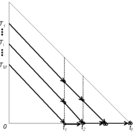
In Section 3.3 and 3.2, we suppose thatN > M. When less than or equal toM tokens only exist, they are always locally feasible by LLREF in the T-L plane.
Theorem 10(Local Feasibility with Small Number of To-kens). WhenN ≤M, tokens are always locally feasible by LLREF.
Proof. We assume that ifN ≤M, then tokens are not lo-cally feasible by LLREF. If it is not lolo-cally feasible, then there should exist at least one critical moment in the T-L plane by Theorem 2. Critical moment implies at least one non-selected token, which contradicts our assumption since all tokens are selectable.
Figure 11:Token Flow whenN≤M
Theorem 10 is illustrated in Figure 11. When the number of tasks is less than the number of processors, LLREF can select all tasks and execute them until their local remaining execution times become zero.
We also observe that at every event B, the number of ac-tive tokens is decreasing. In addition, the number of events B in this case is at mostN, since it cannot exceed the num-ber of tokens. Another observation is that event C never happens whenN ≤M since all tokens are selectable and move diagonally.
Now, we discuss the local feasibility whenN > M.
Theorem 11(Local Feasibility with Large Number of To-kens). WhenN > M, tokens are locally feasible by LLREF ifS0≤M.
Proof. We prove this by induction, based on Theorems 6 and 9. Those basically show that if Sj−1 ≤ M, then
Sj ≤M, wherejis the moment of secondary events. Since we assume thatS0 ≤M,Sj for allj never exceedsM at any secondary event including C and B events. WhenSj
is at mostM for allj, there should be no critical moment in the T-L plane, according to the contraposition of Corol-lary 3. By Theorem 2, no critical moment implies that they are locally feasible.
WhenN(> M)number of tokens are given in the T-L plane and theirS0is less thanM, event C and B occur with-out any critical moment according to Theorem 11. When-ever event B happens, the number of active tokens decreases until there areM remaining active tokens. Then, according to Theorem 10, all tokens are selectable so that they arrive at the rightmost vertex of the T-L plane with consecutive event B’s.
Recall that we consider periodically arriving tasks, and the scheduling objective is to complete all tasks before their deadlines. With continuous T-L planes, if the total utiliza-tion of tasksNi=1uiis less thanM, then tokens are locally feasible in the first T-L plane based on Theorems 10 and 11.
The initialS0for the second consecutive T-L plane is less thanM by Theorem 1 and inductively, LLREF guarantees the local feasibility for every T-L plane, which makes all tasks satisfy their deadlines.
3.5
Algorithm Overhead
One of the main concerns against global scheduling algo-rithms (e.g., LLREF, global EDF) is their overhead caused by frequent scheduler invocations. In [14], Srinivasanet al.
identify three specific overheads:
1. Scheduling overhead, which accounts for the time spent by the scheduling algorithm including that for constructing schedules and ready-queue operations; 2. Context-switching overhead, which accounts for the
time spent in storing the preempted task’s context and loading the selected task’s context; and
3. Cache-related preemption delay, which accounts for the time incurred in recovering from cache misses that a task may suffer when it resumes after a preemption. Note that when a scheduler is invoked, the context-switching overhead and cache-related preemption delay may not happen. Srinivasanet al. also show that the num-ber of task preemptions can be bounded by observing that when a task is scheduled (selected) consecutively for execu-tion, it can be allowed to continue its execution on the same processor. This reduces the number of context-switches and possibility of cache misses. They bound the number of task preemptions under Pfair, illustrating how much a task’s ex-ecution time inflates due to the aforementioned overhead. They show that, for Pfair, the overhead depends on the time quantum size.
In contrast to Pfair, LLREF is free from time quanta. However, it is clear that LLREF yields more frequent sched-uler invocations than global EDF. Note that we use the number of scheduler invocations as a metric for overhead measurement, since it is the scheduler invocation that con-tributes to all three of the overheads previously discussed. We now derive an upper bound for the scheduler invocations under LLREF.
Theorem 12 (Upper-bound on Number of Secondary Events in T-L plane). When tokens are locally feasible in the T-L plane, the number of events in the plane is bounded withinN+ 1.
Proof. We consider two possible cases, when a token Ti hits the NLLD, and it hits the bottom. After Ti hits the NLLD, it should move along the diagonal to the rightmost vertex of the T-L plane, because we assume that they are locally feasible. In this case,Tiraises one secondary event, event C. Note that its final event B at the rightmost vertex occurs together with the next releasing event of another task (i.e., beginning of the new T-L plane). IfTihits the bottom,
then the token becomes inactive and will arrive at the right vertex after a while. In this case, it raises one secondary event, event B. Therefore, eachTican cause one secondary event in the T-L plane. Thus,Nnumber of tokens can cause
N+1number of events, which includesNsecondary events and a task release at the rightmost vertex.
Theorem 13(Upper-bound of LLREF Scheduler Invoca-tion over Time). When tasks can be feasibly scheduled by LLREF, the upper-bound on the number of scheduler invo-cations in a time interval [ts,te] is:
(N+ 1)· 1 +N i=1 t e−ts pi ,
wherepiis the period ofTi.
Proof. Each T-L plane is constructed between two consec-utive events of task release, as shown in Section 2.2. The number of task releases during the time betweentsandteis
N
i=1tep−its. Thus, there can be at most1+
N
i=1tep−its
number of T-L planes betweents and te. Since at most
N+1events can occur in every T-L plane (by Theorem 12), the upper-bound on the scheduler invocations between ts
andteis(N+ 1)·(1 +Ni=1te−ts
pi ).
Theorem 13 shows that the number of scheduler invoca-tions of LLREF is primarily dependent onN and eachpi
— i.e., more number of tasks or more frequent releases of tasks results in increased overhead under LLREF.
3.5.1 Experimental Evaluation
We conducted simulation-based experimental studies to val-idate our analytical results on LLREF’s overhead. We con-sider an SMP machine with four processors. We concon-sider eight tasks running on the system. Their execution times and periods are given in Table 1. The total utilization is ap-proximately 3.72, which is less than 4, the capacity of pro-cessors. Therefore, LLREF can schedule all tasks to meet their deadlines. Note that this task set’sα(i.e.,maxN{ui}) is 0.824, but it does not affect the performance of LLREF, as opposed to that of global EDF.
Table 1:Task Parameters (8 Task Set)
Tasks ci pi ui T1 3 7 0.429 T2 1 16 0.063 T3 5 19 0.263 T4 4 5 0.8 T5 2 26 0.077 T6 15 26 0.577 T7 20 29 0.69 T8 14 17 0.824
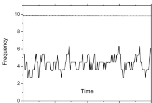
Figure 12:Scheduler Invocation Frequency with 8 Tasks
To evaluate LLREF’s overhead in terms of the number of scheduler invocations, we define the scheduler invocation frequency as the number of scheduler invocations during a time interval ∆t divided by ∆t. We set ∆t as 10. Ac-cording to Theorem 13, the upper-bound on the number of scheduler invocations in this case is(8 + 1)·(1 +10/7+
10/16+ 10/19+10/5+10/26+ 10/26+
10/29+10/17) = 99. Therefore, the upper-bound on the scheduler invocation frequency is 9.9 per tick.
Thus, our experimental results validate our analytical re-sults on LLREF’s overhead.
4
Conclusions and Future Work
We present an optimal real-time scheduling algorithm for multiprocessors, which is not based on time quanta. The algorithm called LLREF, is designed based on our novel technique of using the T-L plane abstraction for reasoning about multiprocessor scheduling. We show that scheduling for multiprocessors can be viewed as repeatedly occurring T-L planes, and correct scheduling on a single T-L plane leads to the optimal solution for all times. We analytically establish the optimality of our algorithm. We also estab-lish that the algorithm overhead is bounded in terms of the number of scheduler invocations, which is validated by our experimental (simulation) results.
We have shown that LLREF guarantees local feasibility in the T-L plane. This result can be intuitively understood in that, the algorithm first selects tokens which appear to be going out of the T-L plane because they are closer to the NLLD.
However, we perceive that there could be other possi-bilities. Theorems 6 and 9 are fundamental steps toward establishing the local feasibility in the T-L plane. We ob-serve that the two theorems’ proofs are directly associated with the LLREF policy in two ways: one is that they de-pend on the critical moment, and the other is that the range allowed forSj−1is computed under the assumption of LL-REF, wherej iscorb. This implies that scheduling
poli-cies other than LLREF may also provide local feasibility, as long as they maintain the critical moment concept. (The range allowed forSj−1could be recomputed for each differ-ent scheduling evdiffer-ent.) The rules of such scheduling policies can include: (1) selecting as many active tokens as possible up toM at every secondary event; and (2) including all to-kens on the NLLD for selection at every secondary event. A good and simple example could be just selecting all to-kens on the NLLD at every event. (i.e., if the number of tokens on the NLLD is less thanM, any token that is not on the NLLD can be selected.) This strategy has the compu-tational complexity reduced as compared to LLREF since it omits the sorting process. Instead, it just needs several queue operations, e.g., to put the tokens on the NLLD into the queue, etc.
When such algorithms can be designed, then tradeoffs can be established between them and LLREF — e.g., on al-gorithm complexity, frequency of event C, etc. Note that even in such cases, the upper-bound of scheduler invoca-tions given in Theorems 12 and 13 hold, because those the-orems are not derived under the assumption of LLREF. De-signing such algorithms is a topic for further study.
We also regard that each task’s scheduling parameters in-cluding execution times and periods are sufficiently longer than the system clock tick, so that they can be assumed as floating point numbers rather than integers. This assump-tion may not be sufficient for the case when task execuassump-tion time is shorter so that integer execution times are a better assumption. However, our intuition strongly suggests that even when task parameters are considered as integers, it should be possible to extend our algorithm to achieve a cer-tain level of optimality—e.g., the error between each task’s deadline and its completion time is bounded within a finite number of clock ticks.
Many other aspects of our task model such as arrival model, time constraints, and execution time model can be relaxed. All these extensions are topics for further study.
5. Acknowledgements
This work was supported by the U.S. Office of Naval Re-search under Grant N00014-00-1-0549 and by The MITRE Corporation under Grant 52917.
References
[1] J. Anderson, V. Bud, and U. C. Devi. An edf-based scheduling algorithm for multiprocessor soft real-time systems. InIEEE ECRTS, pages 199–208, July 2005.
[2] S. Baruah, N. Cohen, C. G. Plaxton, and D. Varvel. Proportionate progress: A notion of fairness in
re-source allocation. InAlgorithmica, volume 15, page 600, 1996.
[3] M. Bertogna, M. Cirinei, and G. Lipari. Improved schedulability analysis of edf on multiprocessor plat-forms. InIEEE ECRTS, pages 209– 218, 2005. [4] J. Carpenter, S. Funk, et al. A categorization of
retime multiprocessor scheduling problems and al-gorithms. In J. Y. Leung, editor, Handbook on Scheduling Algorithms, Methods, and Models, page 30.130.19. Chapman Hall/CRC, Boca Raton, Florida, 2004.
[5] A. Chandra, M. Adler, and P. Shenoy. Dead-line fair scheduling: Bridging the theory and prac-tice of proportionate-fair scheduling in multiprocessor servers. In Proceedings of the 21st IEEE Real-Time Technology and Applications Symposium, 2001. [6] M. L. Dertouzos and A. K. Mok. Multiprocessor
on-line scheduling of hard real-time tasks. IEEE Trans-actions on Software Engineering, 15(12):1497–1506, December 1989.
[7] U. C. Devi and J. Anderson. Tardiness bounds for global edf scheduling on a multiprocessor. In IEEE RTSS, 2005.
[8] S. K. Dhall and C. L. Liu. On a real-time scheduling problem.Operations Research, 26(1):127140, 1978. [9] J. Goossens, S. Funk, and S. Baruah. Priority-driven
scheduling of periodic tasks systems on multiproces-sors. Real-Time Systems, 25(2-3):187–205, 2003. [10] P. Holman and J. Anderson. Adapting pfair scheduling
for symmetric multiprocessors. Journal of Embedded Computing, To appear. Available at: http://www.
cs.unc.edu/˜anderson/papers.html.
[11] K. Lin, Y. Wang, T. Chien, and Y. Yeh. Designing mul-timedia applications on real-time systems with smp ar-chitecture. InIEEE Fourth International Symposium on Multimedia Software Engineering, page 17, 2002. [12] QNX. Symmetric multiprocessing. http://www.
qnx.com/products/rtos/smp.html. Last
accessed October 2005.
[13] A. Srinivasan and S. Baruah. Deadline-based schedul-ing of periodic task systems on multiprocessors. In In-formation Processing Letters, pages 93–98, Nov 2002. [14] A. Srinivasan, P. Holman, J. Anderson, and S. Baruah. The case for fair multiprocessor scheduling. In
IEEE International Parallel and Distributed Process-ing Symposium, page 1143, 2003.