Differentially Private Trajectory Analysis for
Points-of-Interest Recommendation
Chao Li
School of Information Sciences University of Pittsburgh
Pittsburgh, USA Email: [email protected]
Balaji Palanisamy School of Information Sciences
University of Pittsburgh Pittsburgh, USA Email: [email protected]
James Joshi
School of Information Sciences University of Pittsburgh
Pittsburgh, USA Email: [email protected]
Abstract—Ubiquitous deployment of low-cost mobile posi-tioning devices and the widespread use of high-speed wireless networks enable massive collection of large-scale trajectory data of individuals moving on road networks. Trajectory data mining finds numerous applications including understanding users’ historical travel preferences and recommending places of interest to new visitors. Privacy-preserving trajectory mining is an important and challenging problem as exposure of sensitive location information in the trajectories can directly invade the location privacy of the users associated with the trajectories. In this paper, we propose a differentially private trajectory analysis algorithm for points-of-interest recommendation to users that aims at maximizing the accuracy of the recommendation results while protecting the privacy of the exposed trajectories with differential privacy guarantees. Our algorithm first transforms the raw trajectory dataset into a bipartite graph with nodes representing the users and the points-of-interest and the edges representing the visits made by the users to the locations, and then extracts the association matrix representing the bipartite graph to inject carefully calibrated noise to meet -differential privacy guarantees. A post-processing of the perturbed associa-tion matrix is performed to suppress noise prior to performing a Hyperlink-Induced Topic Search (HITS) on the transformed data that generates an ordered list of recommended points-of-interest. Extensive experiments on a real trajectory dataset show that our algorithm is efficient, scalable and demonstrates high recommendation accuracy while meeting the required differential privacy guarantees.
I. INTRODUCTION
Ubiquitous deployment of mobile positioning devices and the widespread use of high-speed wireless networks enable massive collection of large-scale trajectory data of individuals moving on road networks. The rapid proliferation of low-cost GPS-supported mobile devices enables a wide range of based service (LBS) applications including location-based social networks [10], [30], location-location-based advertis-ing [2], [22], location-based information sharadvertis-ing [9], [24] and navigation applications [28], [32]. A trajectory represents a sequence of location information formed by a series of
(latitude, longitude, timestamp) triple that captures a
va-riety of travel information of the users including user’s move-ment pattern [17], travel paths [36] and travel destination [34], [35]. Each travel destination in a trajectory reveals that the user has made a visit to the place. In addition to this information, a trajectory may also include temporal information such as the
visiting times of the users. While trajectories of an individual mobile user can be analyzed to understand her personal travel recommendations comprehensively, aggregate analysis of historical trajectory data belonging to different mobile users can provide more generalized travel recommendations such as ‘Where are the top-10 points-of-interest in a given city?’, ‘Which shopping mall is the most popular in this area?’ and ‘Which users have frequently visited this restaurant?’.
Although historical personal trajectory data provide im-mense information to generate accurate and useful points-of-interest recommendation, the exposure of the sensitive trajectory information can pose significant privacy risks that can invade the location privacy of the users. In particular, the location information of the travel destination, represented as a two-dimensional geographical region, is often associated with a semantic meaning, such as a university, a shopping mall or a hospital. The disclosure of the association between a mobile user and such a location may reveal private information about the health conditions, life style and social and political beliefs of the user. For example, if an adversary infers the association between a user and a treatment center, the health state of the user may be revealed.
Privacy-preserving trajectory mining is an important and challenging problem as exposure of sensitive location informa-tion in the trajectories can directly invade the locainforma-tion privacy of the users associated with the trajectories. Differential pri-vacy [12], [13], as a state-of-the-art pripri-vacy paradigm, provides a model to quantify the disclosure risks by ensuring that the published statistical data does not depend on the presence or absence of an individual record in the dataset. By carefully applying differential privacy mechanisms [12], [13], [25] on trajectory data, the personal trajectory information, such as the travel destination of the users, can be protected from the malicious or curious inference from the recommendation results, thus protecting the location privacy of the mobile users. In this paper, we propose a differentially private trajectory analysis algorithm for points-of-interest recommendation to users that aims at maximizing the accuracy of the recom-mendation results while protecting the privacy of the exposed trajectories with differential privacy guarantees. Our algorithm first transforms the raw trajectory dataset into a bipartite graph with nodes representing the users and the points-of-interest
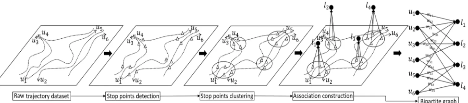
Fig. 1: User-location bipartite graph construction and the edges representing the visits made by the users to the
locations, and then extracts the association matrix representing the bipartite graph to inject carefully calibrated noise to meet
-differential privacy guarantees. A post-processing of the perturbed association matrix is performed to suppress noise prior to performing a Hyperlink-Induced Topic Search (HITS) on the transformed data that generates an ordered list of recommended points-of-interest. We perform extensive exper-iments on the GeolifeGPS trajectory dataset [34], [35], [36] which contains 17621 trajectories collected from 182 users for five years. Our results show that the proposed algorithm is efficient, scalable and demonstrates good recommendation accuracy while guaranteeing differential privacy.
The rest of the paper is organized as follows: We first discuss the related work in Section II. Then, in Section III, we present the definitions of trajectory processing and differential privacy and the model to transfer a raw trajectory dataset to a user-location bipartite graph. In Section IV, we introduce our privacy goal and explain the proposed differentially private trajectory analysis algorithm for travel recommendation. We experimentally evaluate our algorithm in Section V under varying differential privacy budgets, global sensitivity levels and database scale. Finally, we conclude in Section VI.
II. RELATED WORK
Location privacy has been an active research area for a long time. In the past, the location privacy protection mechanisms mainly focused on prevention by protectively processing and perturbing the location information prior to disclosure. De-pending on processing location data discretely or continuously, the location privacy protection mechanisms can be roughly classified to location data perturbation techniques represented by [16], [23], [27], [31], and trajectory inference prevention techniques represented by [3], [4], [5], [6]. The latter can be further broken down into trajectory perturbation [6] and Mix-zone [3], [4], [5] techniques. However, all these techniques assume to restrict the background knowledge of the adver-sary, which fails to provide strong and quantifiable privacy guarantee.
Differential privacy [12], [13], as a state-of-the-art privacy paradigm, provides a model to quantify the disclosure risks by ensuring that the published statistical data does not depend on the presence or absence of an individual record in the dataset. Differential privacy can dispense with the restriction of the adversary background knowledge and quantify the privacy
in a mathematically provable manner. By carefully applying differential privacy mechanisms [12], [13], [25] to the trajec-tory data, the personal trajectrajec-tory information can be protected from malicious inference from the statistical outputs. Usually, the raw trajectory dataset is first transferred to special data structures, such as Prefix tree [8], [19] or N-gram [7]. Then, the differential privacy protection mechanisms (e.g. Laplace Mechanism [12], Exponential Mechanism [25]) inject noises to the data structures before releasing them for further processing. To the best of our knowledge, the work presented in this paper is the first differential privacy protection mechanism aimed at processing trajectories modeled as bipartite graphs to generate accurate travel recommendation while protecting the location privacy of the users in the trajectories.
III. CONCEPTS ANDMODEL
In this section, we first present the background concepts and the bipartite graph model used to model raw trajectory datasets and the user-location associations in the dataset. We then discuss the differential privacy model and mechanisms for achieving differential privacy.
A. User-location bipartite graph representation
The trajectory dataset analysis typically consists of two ma-jor components, namely trajectory preprocessing and trajectory analysis [33]. Depending on the objective of the analysis, the output of trajectory preprocessing can be organized as graphs [34], matrix [35] or tensors [29]. For the purpose of points-of-interest recommendation considered in this work, the raw trajectory dataset is transformed to be processed as a bipartite graph [33]. A bipartite graph can be represented by a graph, G = (U, L, E), containing m = |U| nodes on the left side, n = |L| nodes on the right side and a set of edges E ⊆ U ×L between the two sets of nodes. This structure naturally meets the objectives of the points-of-interest recommendation problem as the left nodes and right nodes can respectively represent users and point-of-interest (POI) locations to be recommended. Here an edgeeij = (ui, lj)∈E indicates that the user ui visited the POI location lj. In addition, we expect to know the frequency of visit between useruiand locationlj modeled as the edge weightwij of the edgeeij.
To construct such a user-location bipartite graph from the raw trajectory dataset, we follow a sequence of three steps as shown in Figure 1. We start from the raw trajectory dataset:
Definition 1 (RAW TRAJECTORY DATASET). The raw trajec-tory dataset RT D = {(ui, T Di)|1 ≤ i ≤ m} contains the
trajectory data (T Di) for m users (ui). The trajectory data
T Di ={(xj, yj, tj)|1 ≤j ≤ki} of user ui is formed by ki
triple, consisting of latitude xj, longitude yj and timestamp
tj (tj< tj+1).
In the example shown in Figure 1, we find the trajectory data for users u1 to u6 as six dotted lines as the trajectory
data is always discretely captured by GPS devices. In the first step, we identify the stop points for all the users. A stop point is defined as a spatial region that the trajectory data fluctuates within a distance thresholdDtfor at least a time thresholdTt.
Definition 2(STOP POINTS SET). The stop points setSP S=
{(ui, SPi)|1 ≤i ≤m} contains the stop points information
(SPi) for the m users (ui). The stop points information
SPi = {spj = (xj, yj)|1 ≤ j ≤ pi} for user ui is
formed by pi stop points. A stop point sp is detected when
a subset of sequential triple of T Di,{(xj, yj, tj)|a≤j≤b}
follows ∀a < j ≤ b, p(xj−xa)2+ (yj−ya)2 ≤ Dt,
p
(xb+1−xa)2+ (yb+1−ya)2> Dt,tb−ta≥Tt.
In Figure 1, the stop points are identified as triangles. Subsequently in the second step, these stop points (triangles) are clustered through well-known clustering techniques such as k-means [15], DBSCAN [14] or OPTICS [1] clustering algorithms. These clustered stop points implicitly recommend those regions covered by the clusters as attractive places as multiple users in the RTD dataset have historically visited (stopped at) them. As can be seen in Figure 1, the stop points of the six users form four clusters, represented by l1
to l4. We denote each cluster as a location as we need to
assign a geographically semantic meaning to the cluster for travel recommendation. In practice, these locations can be represented by the landmarks (e.g. tourist attractions, shopping malls) within the clusters.
Finally, in the third step, we need to construct the as-sociations between the users and the locations to build the user-location bipartite graph. We can connect each stop point with its associated location with an arrow line pointing to the location, which denotes that the user of this stop point has visited the location once. Actually, a user may have more than one stop points within one cluster, which indicates that this user visited this location multiple times. This information, called frequency of visit, is important for travel recommen-dation since a more frequent visit can implicitly represent a stronger recommendation. Therefore, if we denote an edge in the user-location bipartite graph to mean that the user visited the location, we can apply the frequency of visit as the weight of the edge to indicate that the user has visited the location multiple times. Based on this assumption, we define the user-location bipartite graph as:
Definition 3(USER-LOCATION BIPARTITE GRAPH). The user-location bipartite graph U LBG = (U, L, E) consists of the left set of user nodes U = {ui|1 ≤ i ≤ m}, the right set
of location nodes L ={lj|1 ≤j ≤ n} and the set of visits
represented as edgesE={eij = (ui, lj, wij)|1≤i≤m,1≤
j≤n} ⊆U×L, wherewij is the frequency of the visit. We next introduce the notion of differential privacy and the mechanisms required to achieve differential privacy guarantees in a dataset.
B. Differential privacy
Differential privacy is a classical privacy definition [12] that makes conservative assumptions about the adversary’s background knowledge and bounds the allowable error in a quantified manner. In general, differential privacy is designed to protect a single individual’s privacy by considering adjacent data sets which differ only in one record. Before presenting the formal definition of -differential privacy, we first define the notion of adjacent datasets in the context of differential privacy. A data setDcan be considered as a subset of records from the universeU, represented byD∈N|U|, whereNstands for the non-negative set and Di is the number of element
i in N. For example, if U = {a, b, c}, D = {a, b, c} can be represented as {1,1,1} as it contains each element of U
once. Similarly, D0 = {a, c} can be represented as {1,0,1}
as it does not contain b. Based on this representation, it is appropriate to usel1distance (Manhattan distance) to measure
the distance between data sets.
Definition 4 (DIFFERENTIAL PRIVACY [12]). A randomized
algorithm Aguarantees -differential privacy if for all adja-cent datasetsD1 andD2differing by at most one record, and
for all possible resultsS ⊆Range(A),
P r[A(D1) =S]≤e×P r[A(D2) =S]
where the probability space is over the randomness ofA. In other words, the possible results of the randomized algorithm, given a dataset and a query, can form a distribution and differential privacy guarantees that the change of the distribution for two input databases differing in one record is bounded by a threshold. Many randomized algorithms have been proposed to guarantee differential privacy [12], [25]. In our work, we use the most commonly used differential privacy mechanism namely the Laplace Mechanism [12]. Given a data setD, a functionf and the budget, the Laplace Mechanism first calculates the actual f(D) and then perturbs this true answer by adding a carefully calibrated noise [12]. The noise is calculated based on a Laplace random variable, with the variance λ=4f /, where4f is thel1 sensitivity, which is
defined as follows.
Definition 5 (l1 SENSITIVITY [13]). Given a function f :
N|U|→Rd, thel1 sensitivity is measured as:
4f = max
D1,D2∈N|U|
||D1−D2||1=1
||f(D1)−f(D2)||1
where||f(D1)−f(D2)||1=|f(D1)−f(D2)|is the
Manhat-tan DisManhat-tance andU stands for the record universe.
In other words,l1sensitivity measures the maximum impact
Fig. 2: Differentially private bipartite graph mining
is only related to the functionf itself, but independent of the data sets.
Definition 6(LAPLACEMECHANISM[12]). Given a function
f :N|U|→
Rd, a budgetand a data setD, for each output,
ALM(D, f, ) =f(D) +Lap(4f /)
where Lap(4f /) is a random variable sampled from the Laplace distribution with0 mean and4f /variance.
We next discuss the proposed differentially private bipartite graph analysis techniques for trajectory analysis that employs a Laplace Mechanism to achieve differential privacy guarantees in the exposed points-of-interest recommendation.
IV. DIFFERENTIALLYPRIVATETRAJECTORYANALYSIS
The proposed differentially private trajectory analysis tech-nique analyzes the user-location bipartite graph obtained from the raw trajectories to generate a list of ordered recommended locations (points-of-interest) and another list of ordered rec-ommended users based on their frequency of visits to a location. We start from presenting the privacy goal, namely what is identified as a ‘record’ in Definition 4 that needs to be protected by the differential privacy mechanism. We then present the proposed differentially private algorithm for bipartite graph analysis that generates the two recommendation lists from the user-location bipartite graph.
A. Privacy goal
By considering the user-location bipartite graph as a dataset, a ‘record’ in Definition 4 has the form ‘< ui, lj >’, repre-senting user ui visited location lj once, namely a stop point defined in Definition 2. Therefore, an edgeeij = (ui, lj, wij) in the bipartite graph, which can be considered as a group of
wij of (ui, lj,1), results in wij of same < ui, lj > records in the dataset. The entire bipartite graph can be transferred to a dataset with Pm,n
i=1,j=1wij records. Then, by setting the globall1sensitivity4f in Definition 5 to different values, we
can protect different levels of differential privacy. We define
4f ∈[1, wmax], wherewmaxrepresents the maximum weight
among the edges. The proposed differentially private trajectory analysis algorithm with sensitivity 4f ∈ [1, wmax] can thus protect differential privacy of a group of4f records. In other words, the differential privacy of any edge eij = (ui, lj, wij) in the bipartite graph with wij ≤ 4f can be protected. When
4f = 1, the edges withwij = 1, namely the visits that only
happened once, can be protected. When4f =wmax, all the edges in the bipartite graph corresponding to the association between each pair of user and location, can be protected. To sum up, a larger4f results in more noisy edges in the bipartite graph to be protected but results in lower recommendation results due to higher injected noise. We will evaluate the varying4f later in Section V.
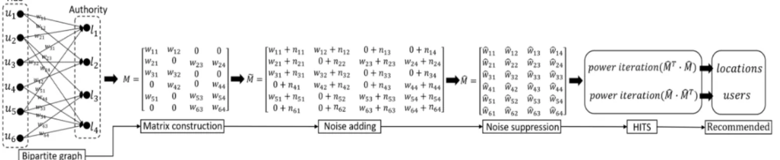
B. Differentially private Points-of-Interest Recommendation Among the recommendation algorithms [11], [20], [26], [35], the one that fits the bipartite graph structure best is the HITS-based algorithm [35]. Hyperlink-Induced Topic Search (HITS) is a link analysis algorithm originally designed for web pages rating [21]. It defines a hub as a web page with many links pointing to other web pages and an authority as a web page pointed by many other web pages. It assumes a good hub points to many good authorities and a good authority is pointed by many good hubs. In the user-location bipartite graph, edges point to locations from users. Therefore, by considering users and locations as hubs and authorities respectively, we can apply HITS algorithm to score every user and location. A user with higher score represents a more experienced user who has more knowledge about the given city and a location with higher score indicates a more popular place that is worth being visited. Therefore, with the user-location bipartite graph as input, we expect the algorithm to output the user and location lists ordered by the scores while preserving differential privacy. We present a pseudocode of the differentially private mining algorithm in Algorithm 1 and illustrate the process in Figure 2.
The differentially private mining algorithm consists of four steps, namely matrix construction (line 1-2), noise addition (line 3-9), noise suppression (line 10) and HITS (line 11-12). In the first step, the bipartite graph structure is transformed into an association matrix M. The matrix M has m = |U|
rows and n =|L| columns. Each entry in M is denoted by the weight wij of the edge between user ui and location lj. If userui never visited locationlj,wij is set to 0.
Then, in the second step, each entry wij is perturbed using noise calculated by Laplace Mechanism [12] to become
e
wij = wij+Lap(4f) so that M becomes Mf. Each noise
is a random variable sampled from Laplace distribution with variance sensitivitybudget . The privacy budgetis typically consid-ered to be 1 in many differential privacy settings [12], [13]. A
Algorithm 1:Differentially private bipartite graph mining
Input :User-location bipartite graphU LBG= (U, L, E), expected privacy levellv∈[1, wmax], budget.
Output:Recommended authority (locations) listA, recommended hub (users) listH.
1 Initialize matrixM[m=|U|][n=|L|],Mf[m][n],Mc[m][n]
with 0s;
2 TransferU LBGto matrixM by fillingM with
{wij|1≤i≤m,1≤j≤n}; 3 4f=lv; 4 δ=4f ; 5 fori= 1to mdo 6 fori= 1to ndo 7 Mf[i][j] =M[i][j] +Lap(δ); 8 end 9 end 10 Mc=Sup(Mf); 11 A=powerIte(McT·Mc); 12 H =powerIte(Mc·McT);
smaller indicates that the difference between the statistical query replies caused by the change of one record in the dataset is smaller, thus providing better privacy protection. We will evaluate the impact of different values of in Section V. In our algorithm, all the entries share the same privacy budget
because of their independence and the composition property of differential privacy:
Theorem 1 (COMPOSITION THEOREM [13]). Let Ai be
i-differential private algorithms applying to independent
datasets Di for i ∈ [1, k]. Then their combination APk i=1
is max(i)-differential private.
The sensitivity 4f can be selected from the range
[1, wmax]. However, we note that the noise can be significantly
high without further post-processing. Due to higher noises, the accuracy of recommendation can actually become too low to be acceptable. Therefore, in the third step, we apply consistency constraints to post-process the matrix from Mf
to Mc to suppress noise and improve the recommendation
accuracy.
Theorem 2 (POST-PROCESSING [13]). Let A be a
-differentially private algorithm andgbe an arbitrary function. Then g(A)is also-differentially private.
We propose three consistency constraints, named zero con-sistency constraint(zero-CC), up concon-sistency constraint (up-CC) and down consistency constraint(down-(up-CC). In zero-CC, since all the entries wij inM are non-negative, the negative
e
wij inMfafter perturbation is constrained to be wbij = 0in
c
M to ensure consistency while the non-negative weij keeps same in Mcas wbij =weij. The up-CC and down-CC follow
the isotonic regression [18]. Specifically, in up-CC, the entries
wij inM are sorted from0towmaxin non-decreasing order. After adding noises to the non-decreasing list of entries, the perturbed entries weij should also keep the non-decreasing order to ensure consistency. If one perturbed entry is smaller
0 10 20 30 40 50 60 70 80 0 10 20 30 40 50 60 70 80 90 100
number
weightFig. 3: Edge weight distribution
than the one before it in the list, this perturbed entry will be adjusted to be equal to the one before it, thus making the list non-decreasing. After adjusting all weij to wbij, the
non-decreasing list is transferred back to matrix, namely Mc. The
down-CC is similar to up-CC, but the list is constrained to follow a non-increasing order fromwmax to0.
Finally, after generatingMc, we apply the HITS algorithm to
calculate the recommended authority (locations) listAand the recommended hub (users) list H. Precisely, we can initialize
AandH to be vectors of1s with sizenandmrespectively. Then, by applying power iteration method [35], we can get the eigenvectors of McT ·McandMc·McT as the final A andH
respectively. We refer the interested readers to [21] for more details on HITS.
V. EXPERIMENTAL EVALUATION
In this section, we experimentally evaluate the performance offered by the proposed differentially private trajectory anal-ysis algorithm. Before reporting our results, we first present our experimental setup.
A. Experimental setup
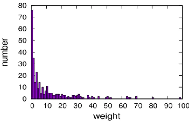
Our experiments were programmed in Java language and implemented on an Intel Core i7 2.70GHz PC with 16GB RAM. In our experiments, we apply theGeolifeGPS trajectory dataset [34], [35], [36], which contains 17621 trajectories collected from 182 users for five years. We first follow the user-location bipartite graph construction scheme shown in Figure 1 to process the raw trajectory dataset and generate the user-location bipartite graph. The sizes of node sets, edge set and stop point set are shown in Table I (some users are abundant during clustering). Each edge in the user-location bipartite graph is assigned a weightwrepresenting the number of visits. The distribution of weights among the 316 edges is shown in Figure 3 (we just show the part forw≤100) and the statistics of weights is shown in Table II. As can be seen, most edges have small weights, indicating that users have many rarely visited locations. This suggests the intuition behind our privacy goal. That is, we can inject little noise to protect most of the edges in the bipartite graph. Typically, these protected edges have lower weights but higher sensitivity.
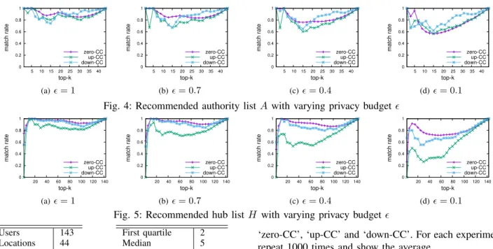
0 0.2 0.4 0.6 0.8 1 5 10 15 20 25 30 35 40 match rate top-k zero-CC up-CC down-CC (a)= 1 0 0.2 0.4 0.6 0.8 1 5 10 15 20 25 30 35 40 match rate top-k zero-CC up-CC down-CC (b)= 0.7 0 0.2 0.4 0.6 0.8 1 5 10 15 20 25 30 35 40 match rate top-k zero-CC up-CC down-CC (c) = 0.4 0 0.2 0.4 0.6 0.8 1 5 10 15 20 25 30 35 40 match rate top-k zero-CC up-CC down-CC (d)= 0.1
Fig. 4: Recommended authority listAwith varying privacy budget
0 0.2 0.4 0.6 0.8 1 20 40 60 80 100 120 140 match rate top-k zero-CC up-CC down-CC (a)= 1 0 0.2 0.4 0.6 0.8 1 20 40 60 80 100 120 140 match rate top-k zero-CC up-CC down-CC (b)= 0.7 0 0.2 0.4 0.6 0.8 1 20 40 60 80 100 120 140 match rate top-k zero-CC up-CC down-CC (c) = 0.4 0 0.2 0.4 0.6 0.8 1 20 40 60 80 100 120 140 match rate top-k zero-CC up-CC down-CC (d)= 0.1
Fig. 5: Recommended hub listH with varying privacy budget
Users 143 Locations 44 Stop points 8017 Edges 316 TABLE I: No. of First quartile 2 Median 5 Third quartile 18 Max 591
TABLE II:w statistics
B. Experimental results
The goal of our experiments is to evaluate the performance of the proposed differentially private user-location bipartite graph analysis algorithm under various privacy budgets and sensitivity values. That is, we evaluate the accuracy of the recommendation results while simultaneously meeting the differential privacy guarantees. We define top-k match rate to measure the recommendation results. If we denote the recommended authority (location) list asA={a1, a2, ..., an} and the recommended hub (user) list asH ={h1, h2, ..., hn}, where the elements with smaller index have higher score, and represent the top-k elements in the list asAk={a1, a2, ..., ak}
and Hk ={h1, h2, ..., hk} respectively, the top-k match rate
forAisM Rk(A) =org(Ak)
Tnoised(A k)
org(Ak) and the top-k match rate for H is M Rk(H) = org(Hk)
Tnoised(H k)
org(Hk) , where org() denotes the original lists without injected noise to protect differential privacy and noised()stands for the differentially private lists with noise. In other words, for a query like ‘show me top-5 recommended locations in this city’, we expect the replied 5 locations do not change after adding noise. Our experiments consist of three components. The noise calibrated by the Laplace mechanismLap(4f)is affected by the two parameters, privacy budget and global sensitivity
4f. Therefore, in the first part, we adjust the privacy budget
to observe the change ofM Rk(A)andM Rk(H). Then, in the second part, we adjust the global sensitivity4f to evaluate the algorithm performance. Finally, to evaluate the scalability of the algorithm, we reduce the raw dataset scale by only using the 100-day trajectory data and only using the first-90-user trajectory data respectively. In all the experiments, we evaluate the three consistency constraint schemes, denoted by
‘zero-CC’, ‘up-CC’ and ‘down-CC’. For each experiment, we repeat 1000 times and show the average.
In the first set of experiments, we change the value of privacy budget from 1 to 0.7, 0.4 and 0.1 and show the results with varying k of M Rk(A)and M Rk(H) as Figure 4 and Figure 5 respectively. In differential privacy, a smaller privacy budget means the difference between query replies from two datasets differing in at most one record is smaller, which implies higher privacy requirement and requires more noise to guarantee better privacy protection. For this part, we fix the global sensitivity to be 1 to protect differential privacy of individual stop point or the 76 weight-1 edges. When
= 1, Figure 4(a) and Figure 5(a) show that for most values of k, M Rk(A) and M Rk(H) for all the three consistency constraint schemes are larger than 80%. If we keep choosing the consistency constraint scheme giving the best results, the match rates can even be larger than 90%. As= 1is typical in most differential privacy settings [12], [13], the 90% accuracy shows that our differentially private bipartite graph analysis algorithm for travel recommendation is practical and effective. In Figure 4(a), we can see that zero-CC provides best match rate whenk≤20, which is defeated by down-CC fork >20. In Figure 5(a), although down-CC is very close to zero-CC, zero-CC gives best results for nearly all the values of k. In both the two figures, up-CC shows worst performance. All the above observations can be explained by the principles of the three consistency constraint schemes and the features of the dataset. The matrix M (input of HITS algorithm) is sparse because most of its entries are 0, indicating no edge between corresponding user and location. In Figure 3, we see that most edges have very small weights and only a small number of edges have outstanding weights. Therefore, the entries inM
can be divided into three classes, entries with high weights, entries with low weights and entries with 0 weights. After adding noise to each entry, the perturbed low-weight entries (e.g. w = 1 +noise) are almost indistinguishable from the perturbed 0-weight entries (e.g. w = 0 + noise), but the perturbed high-weight entries (e.g. w = 100 +noise) still
0 0.2 0.4 0.6 0.8 1 5 10 15 20 25 30 35 40 match rate top-k zero-CC up-CC down-CC (a)4f= 2 0 0.2 0.4 0.6 0.8 1 5 10 15 20 25 30 35 40 match rate top-k zero-CC up-CC down-CC (b)4f= 5 0 0.2 0.4 0.6 0.8 1 5 10 15 20 25 30 35 40 match rate top-k zero-CC up-CC down-CC (c)4f= 18 0 0.2 0.4 0.6 0.8 1 5 10 15 20 25 30 35 40 match rate top-k zero-CC up-CC down-CC (d)4f= 591
Fig. 6: Recommended authority listAwith varying sensitivity 4f
0 0.2 0.4 0.6 0.8 1 20 40 60 80 100 120 140 match rate top-k zero-CC up-CC down-CC (a)4f= 2 0 0.2 0.4 0.6 0.8 1 20 40 60 80 100 120 140 match rate top-k zero-CC up-CC down-CC (b)4f= 5 0 0.2 0.4 0.6 0.8 1 20 40 60 80 100 120 140 match rate top-k zero-CC up-CC down-CC (c)4f= 18 0 0.2 0.4 0.6 0.8 1 20 40 60 80 100 120 140 match rate top-k zero-CC up-CC down-CC (d)4f= 591
Fig. 7: Recommended hub listH with varying sensitivity 4f
0 0.2 0.4 0.6 0.8 1 5 10 15 20 25 30 35 match rate top-k zero-CC up-CC down-CC (a) M Rk(A), 100 days 0 0.2 0.4 0.6 0.8 1 20 40 60 80 100 120 match rate top-k zero-CC up-CC down-CC (b)M Rk(H), 100 days 0 0.2 0.4 0.6 0.8 1 5 10 15 20 25 30 match rate top-k zero-CC up-CC down-CC (c)M Rk(A), 90 users 0 0.2 0.4 0.6 0.8 1 10 20 30 40 50 60 70 match rate top-k zero-CC up-CC down-CC (d)M Rk(H), 90 users
Fig. 8: Varying scalability have outstanding weights. In noise suppression, the zero-CC
tends to makew= 0−noisetow= 0and has little influence to the high-weight entries, low-weight entries and difference between low-weight entries and 0-weight entries. Both the up-CC and down-up-CC have greater influence to the high-weight entries and low-weight entries (makes their order changed). Also, the up-CC reduces the difference between low-weight entries and 0-weight entries while down-CC increases the difference by making w = 0 +noise to w = 0. In HITS, if a user or location is linked by more edges with high weights, it has more chance to be recommended. In Figure 4(a), the locations can be divided into two sets. The first set of locations has higher scores determined by high-weight entries and low-weight entries while the second set of locations have lower scores determined by low-weight entries and 0-weight entries. Therefore, zero-CC, which has little influence to the high-weight entries and low-weight entries, dominates the first set while down-CC, which makes low-weight entries distinguishable from 0-weight entries, dominates the second set. The handover point between zero-CC and down-CC grad-ually decreases from 20 when = 1 to 9 when = 0.1
as shown in Figure 4(b) to 4(d). In Figure 5(a), unlike the locations, most users visited the very popular locations, so their scores are mainly affected by the high-weight entries and low-weight entries, which makes zero-CC to dominate the entire set. The reduction of from Figure 5(b) to 5(d) only makes the advantage of zero-CC more transparent. To sum up, we recommend zero-CC as default consistency scheme for 4f = 1 case.
In the second set of experiments, we adjust the global sensitivity4f from 2 to 5, 18 and 591 and show the results with varying k of M Rk(A) and M Rk(H) in Figure 6 and Figure 7 respectively. The selected sensitivities are the first quartile, median, third quartile and max of weight w in its distribution, shown in Table II and Figure 3, which can protect 1/4, 1/2, 3/4 and all edges in the bipartite graph respectively. In this part, the objective is to evaluate the algorithm performance with varying sensitivity and fixed = 1. As can be seen, we can achieve about 80%, 60%, 50% and 40% match rate for all values ofkto protect 1/4, 1/2, 3/4 and all edges. Surprisingly, our algorithm still achieves 40% match rate for our ultimate privacy goal. However, in most cases, we recommend setting
4f = 1to protect the 23.4% weight-1 edges and have match rate higher than 90%. In addition, we find that when 4f
is large in Figure 6(c), 6(d), 7(c) and 7(d), the down-CC beats zero-CC. A big sensitivity results in a huge injected noise, which makes the perturbed high-weight entries start to be indistinguishable from the perturbed low-weight entries. The zero-CC has little influence to this while the down-CC can again make the perturbed high-weight entries start distinguishable from the perturbed low-weight entries start, thus dominating the entire set. To sum up, for very large sensitivity4f, we recommend the down-CC.
Finally, in the last set of experiments, we change the scale of the dataset to evaluate the performance of our algorithm over databases with different size. We first limit the timestamp of trajectory data from 5 years to the first 100 days and show the results of M Rk(A) andM Rk(H) with = 1 and
4f = 1 in Figure 8(a) and Figure 8(b) respectively. The new user-location bipartite graph contains 123 users and 39 locations. As can be seen, both the M Rk(A)and M Rk(H) become worse, compared with Figure 4(a) and 5(a). Then, we limit the user number from 182 to 90 and show the results of M Rk(A) andM Rk(H) with = 1 and4f = 1 in Figure 8(c) and Figure 8(d) respectively. The new user-location bipartite graph contains 78 users and 31 user-locations. As can be seen, compared with Figure 4(a) and 5(a), the
M Rk(A) becomes worse while M Rk(H) becomes slightly better. From the results, we can see that the data volume does impact the accuracy of recommendation. Specifically, the track of individuals for a longer period of time can help to improve the accuracy of recommendation in terms of both users and locations. However, a dataset with more users can only enhance the accuracy for location recommendation, but reduce the accuracy for user recommendation.
VI. CONCLUSION
In this paper, we propose a differentially private trajectory analysis algorithm for travel recommendation that aims at increasing the accuracy of the recommendation results while protecting the differential privacy of the trajectory data. The proposed approach transforms the raw trajectory dataset into a user-location bipartite graph and injects a carefully calibrated noise to meet the required differential privacy guarantees. We propose three consistency constraint schemes to suppress the noise added in the process which improves the accuracy of the obtained recommendation results. Our extensive experiments on a real trajectory dataset show that our algorithm is efficient, scalable and demonstrates good recommendation accuracy while meeting the required differential privacy guarantees.
ACKNOWLEDGMENT
This work was performed under a partial support by the National Science Foundation under the grant DGE-1438809.
REFERENCES
[1] Ankerst, Mihael,et al. OPTICS: ordering points to identify the clustering structure.ACM Sigmod record, Vol. 28. No. 2. ACM, 1999.
[2] Banerjee, Syagnik Sy, and Ruby Roy Dholakia. Mobile advertising: Does location based advertising work?. 2008.
[3] B. Palanisamy and L. Liu. Attack-resilient mix-zones over road networks: architecture and algorithms. IEEE Transactions on Mobile Computing (TMC 2015), 14(3), 495-508.
[4] B. Palanisamy, L. Liu. Mobimix: Protecting location privacy with mix-zones over road networks. in27th International Conference on Data Engineering (ICDE 2011), 494-505.
[5] A. Beresford and F. Stajano. Location Privacy in Pervasive Computing (2003). inPervasive Computing, 46-55.
[6] Cicek, A. Ercument, Mehmet Ercan Nergiz, and Yucel Saygin Ensuring location diversity in privacy-preserving spatio-temporal data publishing.
The VLDB Journal, 23.4 (2014): 609-625.
[7] Chen, Rui, Gergely Acs, and Claude Castelluccia. Differentially private sequential data publication via variable-length n-grams.Proceedings of the 2012 ACM conference on Computer and communications security, ACM, 2012.
[8] Chen, Rui, et al. Differentially private transit data publication: a case study on the montreal transportation system. Proceedings of the 18th ACM SIGKDD international conference on Knowledge discovery and data mining, ACM, 2012.
[9] Cheng, Zhiyuan, et al. Exploring millions of footprints in location sharing services. ICWSM 2011, (2011): 81-88.
[10] Cho, Eunjoon, Seth A. Myers, and Jure Leskovec. Friendship and mobility: user movement in location-based social networks.Proceedings of the 17th ACM SIGKDD, ACM, 2011.
[11] Dai, Jian,et al. Personalized route recommendation using big trajectory data. Data Engineering (ICDE), 2015 IEEE 31st International Confer-ence on, IEEE, 2015.
[12] Dwork C, McSherry F, Nissim K,et al. Calibrating noise to sensitivity in private data analysis. Theory of cryptography, Springer Berlin Heidelberg, 265-284, 2006.
[13] Dwork C, Roth A. The algorithmic foundations of differential privacy.
Theoretical Computer Science, 9(3-4), 211-407, 2013.
[14] Ester, Martin,et al. A density-based algorithm for discovering clusters in large spatial databases with noise. Kdd, Vol. 96. No. 34. 1996. [15] Forgy, Edward W. Cluster analysis of multivariate data: efficiency versus
interpretability of classifications. Biometrics, 21 (1965): 768-769. [16] B. Gedik, L. Liu. A customizable k-anonymity model for protecting
location privacy, 2004.
[17] Giannotti, Fosca,et al. Trajectory pattern mining. Proceedings of the 13th ACM SIGKDD international conference on Knowledge discovery and data mining, ACM, 2007.
[18] Hay, Michael, et al. Accurate estimation of the degree distribution of private networks. Data Mining, 2009. ICDM’09. Ninth IEEE International Conference on, IEEE, 2009.
[19] He, Xi, et al. Dpt: Differentially private trajectory synthesis using hierarchical reference systems. Proceedings of the VLDB Endowment, 8.11 (2015): 1154-1165.
[20] Ho, Shen-Shyang, and Shuhua Ruan. Preserving privacy for interesting location pattern mining from trajectory data. 2013.
[21] Kleinberg, Jon M. Authoritative sources in a hyperlinked environment.
Journal of the ACM (JACM), 46.5 (1999): 604-632.
[22] Klmel, Bernhard, and Spiros Alexakis. Location based advertising.
Mobile Business, 2002.
[23] Li Chao, and Balaji Palanisamy. ReverseCloak: Protecting Multi-level Location Privacy over Road Networks. in Proc. of 24th ACM International Conference on Information and Knowledge Management (CIKM), 2015.
[24] Li, Nan, and Guanling Chen. Sharing location in online social networks.
IEEE network, 24.5 (2010).
[25] McSherry, Frank, and Kunal Talwar. Mechanism design via differential privacy. FOCS’07, 48th Annual IEEE Symposium on. IEEE, 2007. [26] McSherry, Frank, and Ilya Mironov. Differentially private recommender
systems: building privacy into the net. Proceedings of the 15th ACM SIGKDD international conference on Knowledge discovery and data mining, 2009.
[27] M.F. Mokbel, C.Y. Chow, W.G. Aref. The new Casper:query processing for location services without compromising privacy.VLDB Endowment (2006), 763-774.
[28] Schiller, Jochen, and Agns Voisard, eds. Location-based services. Elsevier. Elsevier, 2004.
[29] Wang, Yilun, Yu Zheng, and Yexiang Xue. Travel time estimation of a path using sparse trajectories. Proceedings of the 20th ACM SIGKDD, ACM, 2014.
[30] Ye, Mao, Peifeng Yin, and Wang-Chien Lee. Location recommendation for location-based social networks. Proceedings of the 18th SIGSPA-TIAL, ACM, 2010.
[31] Z. Xiao, X. Meng, J. Xu. Quality aware privacy protection for location-based services.Advances in Databases: Concepts, Systems and Applications (2007), Springer Berlin Heidelberg, 434-446.
[32] Zhao, Yilin. Vehicle location and navigation systems. 1997.
[33] Zheng, Yu. Trajectory data mining: an overview.ACM Transactions on Intelligent Systems and Technology (TIST), 6.3 (2015): 29.
[34] Zheng, Yu,et al. Mining interesting locations and travel sequences from GPS trajectories. Proceedings of the 18th international conference on World wide web, ACM, 2009.
[35] Zheng, Yu, and Xing Xie. Learning travel recommendations from user-generated GPS traces. ACM Transactions on Intelligent Systems and Technology (TIST), 2.1 (2011): 2.
[36] Zheng, Yu, Xing Xie, and Wei-Ying Ma. GeoLife: A Collaborative Social Networking Service among User, Location and Trajectory.IEEE Data Eng. Bull., 33.2 (2010): 32-39.