biclustermd: An R Package for Biclustering with Missing Values

(1)

2019

biclustermd: An R Package for Biclustering with Missing Values

John Reisner

Iowa State University

Hieu Pham

Iowa State University

Sigurdur Olafsson

Iowa State University, [email protected]

Stephen B. Vardeman

Iowa State University, [email protected]

Jing Li

Boehringer Ingelheim Animal Health

Follow this and additional works at:

https://lib.dr.iastate.edu/imse_pubs

Part of the

Operations Research, Systems Engineering and Industrial Engineering Commons

, and the

Statistics and Probability Commons

The complete bibliographic information for this item can be found at https://lib.dr.iastate.edu/

imse_pubs/225. For information on how to cite this item, please visit http://lib.dr.iastate.edu/

howtocite.html.

This Article is brought to you for free and open access by the Industrial and Manufacturing Systems Engineering at Iowa State University Digital Repository. It has been accepted for inclusion in Industrial and Manufacturing Systems Engineering Publications by an authorized administrator of Iowa State University Digital Repository. For more information, please contact [email protected].

(2)

Abstract

Biclustering is a statistical learning technique that attempts to find homogeneous partitions of rows and

columns of a data matrix. For example, movie ratings might be biclustered to group both raters and

movies. biclust is a current R package allowing users to implement a variety of biclustering algorithms.

However, its algorithms do not allow the data matrix to have missing values. We provide a new R package,

biclustermd, which allows users to perform biclustering on numeric data even in the presence of missing

values.

Disciplines

Operations Research, Systems Engineering and Industrial Engineering | Statistics and Probability

Comments

This is a manuscript of an article published as Reisner, John, Hieu Pham, Sigurdur Olafsson, Stephen

Vardeman, and Jing Li. "biclustermd: An R Package for Biclustering with Missing Values." (2019). Posted

with permission.

Creative Commons License

This work is licensed under a

Creative Commons Attribution 4.0 License

.

(3)

biclustermd: An R Package for

Biclustering with Missing Values

by John Reisner, Hieu Pham, Sigurdur Olafsson, Stephen Vardeman and Jing Li

Abstract Biclustering is a statistical learning technique that attempts to find homogeneous partitions of rows and columns of a data matrix. For example, movie ratings might be biclustered to group both raters and movies.biclustis a current R package allowing users to implement a variety of biclustering algorithms. However, its algorithms do not allow the data matrix to have missing values. We provide a new R package,biclustermd, which allows users to perform biclustering on numeric data even in the presence of missing values.

Introduction

Traditional (one-way) clustering (such as with complete-link hierarchical clustering or k-means) aims to partition only rows (or columns) of a data matrix into homogeneous subsets. Rows or columns are clustered simply based upon their relational similarity to other observations. Biclustering simultaneously groups rows and columns to identify homogeneous “cells”. Biclustering is known to be NP-hard; as such, every existing algorithm approaches this problem heuristically. This methodology was first investigated byHartigan(1972) but was not given much attention until applied to gene expression data (Cheng and Church,2000). Today, biclustering is applied across many areas such as biomedicine, text mining, and marketing (Busygin et al.,2008).

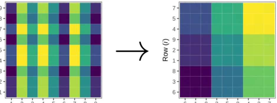
For our purposes, we consider rearranging a data matrix to obtain a checkerboard-like structure where each cell is as homogeneous as possible. In this regard, our algorithm has the same goal as spectral biclustering (Kluger et al.,2003), but approaches the problem in a different way. In contrast to clustering with the end goal being a checkerboard-like structure, other techniques have been proposed based on the singular value decomposition (Lazzeroni and Owen,2002;Bergmann et al.,2003) and others are based on a graph-theoretic approach (Tan and Witten,2014). Although each technique is different, each has the goal of finding substructure within the data matrix. In Figure1we provide a visual suggestion of our biclustering goal. The color scheme represents similar numeric values and our goal is to rearrange the data matrix so that these values form homogeneous cells.

1 2 3 4 5 6 7 8 9 1 2 3 4 5 6 7 8 9 Column (j ) Ro w ( i)

Raw Data Matrix

→

6 3 8 1 2 9 4 5 7 6 1 9 3 5 8 4 2 7 Column (j ) Ro w ( i)

Shuffled Data Matrix

Figure 1:Biclustering withcheckerboard-likestructure

A publicly available R package for biclustering isbiclustbyKaiser and Leisch(2008). This appears to be a commonly used package developed with the intent of allowing users to choose from a variety of algorithms and renderable visualizations. Other biclustering packages includesuperbiclust,iBBiG QUBIC,s4vd,BiBitRwhich each provide unique algorithms and implementations (Khamiakova,

2014;Gusenleitner and Culhane,2019;Zhang et al.,2017;Sill and Kaiser,2015;Ewoud,2017). However, from an implementation and algorithmic standpoint, the methods implemented in these packages fail when given a data matrix with missing values. This is clearly a limitation since there exist many rectangular datasets with missing values. For handling missing data, many imputation methods exist in the literature. While this does produce a complete two-way data table, which can subsequently be fully analyzed using existing biclustering algorithms, it has inherent limitations. When large percentages of data are missing, such as is, for example, common in plant breeding and movie rating applications to be discussed later, it is difficult and impossible to reasonably infer missing values.

(4)

Even if a small number of values are missing values those are potentially missing not-at-random due to non-random and unknown devices. For example, in plant breeding, observation may be missing because it is unreasonable to plant a crop in a particular environment or simply because a plant breeder decides to not plant in certain environments. In these cases, imputing missing values would imply that one can confidently estimate the performance of (say) crop yield in an environment where it was never observed growing. There is a large body of literature on the difficult nature of this problem. With this as motivation, our goal was to produce a biclustering algorithm which can successfully deal with data with missing values without applying imputation or making any assumptions about why data are missing.

Biclustering with missing data

The package described in this paper,biclustermd, implements the biclustering algorithm ofLi et al.

(2020) and their paper gives a thorough explanation of the proposed biclustering algorithm as well as its applicability. For completeness we give an overview of their algorithm here.

Notation

• Xis a data matrix withIrows andJcolumns.Xijis a response measure of rowiin columnjfor

i∈ {1, 2, . . . ,I}andj∈ {1, 2, . . . ,J}.

• Row index setI ={1, 2, . . . ,I}is partitioned intormutually exclusive and exhaustive sets T1,T2, . . . ,Tr.Q ≡partition of the row index set.

• Column index setJ ={1, 2, . . . ,J}is partitioned intocmutually exclusive and exhaustive sets S1,S2, . . . ,Sc.P ≡partition of the column index set.

Our goal for biclustering is to generate a rearranged data matrix with a checkerboard structure such that each “cell” of the matrix defined byQandPis as homogeneous as possible. Depending on specifics of a real problem, “homogeneous” can have different subject matter meanings, and hence optimization of different objective functions can be appropriate. We present our algorithm here with the goal of optimizing a total within-cluster sum of squares given both the row groups inQand column groups inP. This can be interpreted as the total sum of squared errors between cell means and data values within cells. Hence we refer to this as SSE. Using the above notations we haverrow groups (or row clusters) andccolumn groups (or column clusters). LetAdenote anr×c“cell-average matrix” with entries

Amn≡ 1

|{Xij:i∈Tm; j∈Sn; Xij6=N A}|_{_X

∑

ij:i∈Tm;j∈Sn;Xij6=N A}

Xij (1)

form∈1, 2, . . . ,randn∈1, 2, . . . ,c. Here,|·|is the set cardinality function andNAdenotes a missing value. Then, the within-cluster sum of squares function to be minimized is

SSE≡

∑

m,n Xij

∑

6=N A i∈Tm j∈Sn Xij−Amn 2 . (2)

Biclustering with missing data algorithm

1. Randomly generate initial partitionsQ(0)_and_P(0)_{with respectively}_r_{row groups and}_c_column

groups.

2. Create a matrixA(0)_{using Equation (}₁_{) and the initial partitions. In the event that a “cell”}₍_m_,_n₎

defined by{(i,j)|i∈Tmandj∈Sn}is empty,Amncan be set to some pre-specified constant

or some function of the numerical values corresponding to the non-empty cells created by the partition. (For example, the mean of the values coming from non-empty cells in rowmor in columnncan be used.) This algorithmic step should not be seen as imputation of responses for the cell under consideration, but rather only a device to keep the algorithm running.

3. At iterationsof the algorithm, with partitionsP(s−1)_and_Q(s−1)_{and corresponding matrix}

A(s−1)in hand, fori=1, 2, . . . ,Ilet

MR_in= 1 n j∈Sn|Xij6=N A o

∑

j∈Sn s.t.Xij6=N A Xij

(5)

for eachn=1, 2, . . . ,cand compute form=1, 2, . . . ,r d_imR = c

∑

n=1 Amn−MinR 2 · n j∈Sn|Xij6=N A o .

Then createQ(s)∗_{by assigning each row}_i_to_T

mwith minimumdR_im.

4. If forQ(s)∗_every_T

mis non-empty, proceed to Step 5. If at least oneTm=∅do the following:

(a) Randomly choose a row groupTm0with|T_m0|>kR

min(a user-specified positive integer

parameter) and choosekRmove<kRminrow indices to move to one emptyTm. Choose those

indicesifromTm0with the largestkR_movecorresponding values of the sum of squares

c

∑

n=1 j

∑

∈Sn s.t.Xij6=N A Xij−MRin 2 .

(b) If after the move in (a) no empty row group remains, proceed to Step 5. Otherwise return to (a).

5. ReplaceQ(s−1)_{in Step 3 with the updated version of}_Q(s)∗_{and cycle through Steps 3 and 4}

α

times, whereαis a user-specified integer parameter.Ifrow_shuffles>1, replaceQ(s−1)in 3.

with the updated version ofQ(s)∗and cycle through steps 3. and 4.row_shuffles−1times.

6. SetQ(s)₌_Q(s)∗_{. Then update}_A(s−1)_to_A(s)∗_{using the partitions}_Q(s)_and_P(s−1)_{in Equation}

(1). 7. Forj=1, 2, . . . ,Jlet MC_jm= 1 n i∈Tm|Xij6=N A o

∑

i∈Tm s.t.Xij6=N A Xij

for eachm=1, 2, . . . ,rand compute forn=1, 2, . . . ,c dC_jn= r

∑

m=1 Amn−MCjm 2 · n i∈Tm|Xij6=N A o .

Then createP(s)∗_{by assigning each column}_j_to_S

nwith minimumdC_jn.

8. If forP(s)∗_every_S

nis non-empty, proceed to Step 9. If at least oneSn=∅do the following:

(a) Randomly choose a column groupSn0with|S_n0|>kC

min(a user-specified positive integer

parameter) and choosekCmove<kCmincolumn indices to move to one emptySn. Choose

those indicesjfromSn0with the largestkC_movecorresponding values of the sum of squares

r

∑

m=1 i∈

∑

Tm s.t.Xij6=N A Xij−MCjm 2 .

(b) If after the move in (a) no empty column group remains, proceed to Step 9. Otherwise return to (a).

9. ReplaceP(s−1)_{in Step 3 with the updated version of}_P(s)∗_{and cycle through Steps 7 and 8}

β

times, whereβis a user-specified integer parameter. Ifcol_shuffles>1, replaceP(s−1)in 3.

with the updated version ofP(s)∗_{and cycle through steps 7. and 8.}_{col_shuffles}₋_{1 times.}

10. SetP(s) ₌_P(s)∗_{and we have new partitions}_Q(s)_and_P(s)_{. Then update}_A(s)∗_to_A(s)_using

the partitionsQ(s)_and_P(s)_{in Equation (}₁_).

11. Steps 3–10 are executedNtimes or until the algorithm converges, which is when the Rand Indices for successive row and column partitions are both 1. (See the description of the Rand Index below.)

Intuitively, our proposed algorithm is nothing more than a rearrangement of rows and columns with the objective to minimize the objectives given in Steps 3 and 7. We consider Step 1 (the random generation of initial cluster assignments) to be of high importance to avoid any bias in the original structure of the data. As a quantitative way to measure the effectiveness of our biclustering, we consider the sum of squared errors (SSE) as the measure of within cell homogeneity. Paired with the SSE, we allow for three different convergence criteria, the Rand Index (Rand,1971), the Adjusted Rand Index (Hubert and Arabie,1985), and the Jaccard Index (Goodall,1966). These indices provide measures for the similarity between two clusterings.

(6)

Overview of biclustermd

Thebiclustermdpackage consists of six main functions with the most important beingbicluster(). This function is where the algorithmic process is embedded and contains numerous tunable parame-ters.

• data: dataset to bicluster. Must be a data matrix/table with only numbers and missing values in the dataset. It should have row names and column names.

• row_clusters: The number of clusters to partition the rows into. Default isj√Ik • col_clusters: The number of clusters to partition the columns into. Default is√

J

• missing_val: Value or function used to represent empty cells of the data matrix. If a value, a random normal variable centered at itself with standard deviationmiss_val_sdis used each iteration. Note that this is not data imputation but a temporary value used by the algorithm. • missing_val_sd: Standard deviation of the normal distributionmiss_valfollows ifmiss_valis

a number. By default this equals 1.

• similarity: The metric used to compare two successive clusterings. Can be "Rand" (default), "HA" for the Hubert and Arabie adjusted Rand index or "Jaccard". Seecluesfor details. • row_min_num: Minimum row cluster size in order to be eligible to be chosen when filling an

empty row cluster. Default isbI/rc.

• col_min_num: Minimum column cluster size in order to be eligible to be chosen when filling an empty column cluster. Default isbJ/cc.

• row_num_to_move: Number of rows to remove from the sampled cluster to put in an empty row cluster. Default is 1.

• col_num_to_move: Number of columns to remove from the sampled cluster to put in an empty column cluster. Default is 1.

• row_shuffles: Number of times to shuffle rows in each iteration. Default is 1. • col_shuffles: Number of times to shuffle columns in each iteration. Default is 1. • max.iter: Maximum number of iterations to let the algorithm run.

• verbose: Logical. If TRUE, will report iteration progress.

In the following sections, we provide an overview of the functionality ofbiclustermd. For the first dataset, we display the array of visualizations available, in the second example we demonstrate the impact of numerous tunable parameters, our final example demonstrates the computational times of our algorithm.

Example with NYCflights13

For a first example, we will utilize the flights dataset from Wickham’s packagenycflights13(Wickham,

2017). Per the package documentation,flightscontains data on all flights in 2013 that departed NYC via JFK, LaGuardia, or Newark. The variables of interest aremonth,dest, andarr_delaythese are the rows, columns and response value, respectively. In a dataset such as this, an application of biclustering would be to determine if there exist subsets of months and airports with similar numbers of delays. From a pragmatic perspective, this discovery may allow for air officials to investigate the connection between these airports and months and why delays are occurring.

Using functions fromtidyverse(?), we generate a two-way data table such that rows represent months, columns represent destination airports, and the numeric response values are the average arrival delays in minutes. This data matrix contains 12 rows (months), 105 columns (destination airports), and approximately 11.7% missing observations. Below is a snippet of our data matrix.

> flights[1:5,1:5]

ABQ ACK ALB ANC ATL

January NA NA 35.17460 NA 4.152047

February NA NA 17.38889 NA 5.174092

March NA NA 17.16667 NA 7.029286

April 12.222222 NA 18.00000 NA 11.724280

(7)

The first step is to determine the number of clusters for months and the number of clusters for destination airports. Since we are clustering months, in this analysis, choosingr =4 row clusters seems reasonable (create a group for each season/quarter of the year). Although this is arbitrary, we choosec=6 column clusters. Since this algorithm incorporates purposeful randomness (by row and column cluster initialization),biclustermd()should be run multiple times keeping the result with the lowest sum of squared errors (SSE) since it may be expected that for different initialization one can obtain a different local minimum (Li et al.,2020).

> bc <- biclustermd(data = flights, col_clusters = 6, row_clusters = 4,

+ miss_val = mean(flights, na.rm = TRUE), miss_val_sd = 1,

+ col_min_num = 5, row_min_num = 3,

+ col_num_to_move = 1, row_num_to_move = 1,

+ col_shuffles = 1, row_shuffles = 1,

+ max.iter = 100)

> bc

Data has 1260 values, 11.75% of which are missing 10 Iterations

Initial SSE = 186445; Final SSE = 82490

Rand similarity used; Indices: Columns (P) = 1, Rows (Q) = 1

The output ofbiclustermd()is a list of class “biclustermd” and “list” containing the following: • The two-way table of data provided to the function.

• The final column and row partition matrices. • SSE generated from the initial partitioning.

• SSE of each iteration, as an “biclustermd_sse” object.

• Similarity measures for rows and columns for each iteration, as an “biclustermd_sim” object. • The number of iterations to convergence.

• A table of resulting cell means.

Analyzing the NYCflights13 biclustering

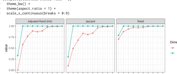
The list output ofbiclustermd()is used for rendering plots and to obtain cell information. One such visual aid is a plot of the convergence indices versus iteration, given in Figure2. From this graphic, we can determine the rate at which convergence occurs for both row and column clusters. Moreover, this provides confirmation that our algorithm can indeed achieve good clusterings along both dimen-sions. Plotting of the similarity measures and SSE is done withautoplot.biclustermd_sim()and

autoplot.biclustermd_sse(), methods added toautoplot()ofggplot2(Wickham,2009).

> autoplot(bc$Similarities, ncol = 3) + + theme_bw() + + theme(aspect.ratio = 1) + + scale_x_continuous(breaks = 0:9) ● ● ● ● _● ● ● ● ● ● ● ● ● ● ● ● ● ● ● ● ● ● ● ● ● ● ● ● ● ● ● ● ● ● ● ● ● ● ● ● ● ● ● ● ● ● ● ● ● ● ● ● ● ● ● ● ● ● ● ●

Adjusted Rand (HA) Jaccard Rand

0 1 2 3 4 5 6 7 8 9 0 1 2 3 4 5 6 7 8 9 0 1 2 3 4 5 6 7 8 9 0.00 0.25 0.50 0.75 1.00 Iteration v alue Dimension ● ● Column Row

Figure 2:Plot of similarity measures for the flights biclustering

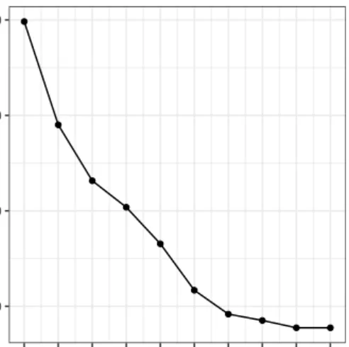
In addition to the similarity plots, one can utilize the SSE graphic as an indication of convergence to a (local) minimum biclustering. This can be seen in Figure3. From this we can observe the rate of

(8)

decrease of the SSE as well as the relative difference between the first and final iteration. Observing closely each of the three convergence criteria suddenly decrease in value along the columns, namely from iteration three to four. The algorithm is simply (attempting to) obtain a lower SSE which may result in column shuffles which differ from iteration to iteration.

> autoplot(bc$SSE) + + theme_bw() + + theme(aspect.ratio = 1) + + scale_y_continuous(labels = comma) + + scale_x_continuous(breaks = 0:9) ● ● ● ● ● ● ● ● ● ● 85,000 90,000 95,000 100,000 0 1 2 3 4 5 6 7 8 9 Iteration SSE

Figure 3:SSE plot of flights biclustering

Traditionally visualizations of biclustering plots are in a heat map fashion.autoplot.biclustermd() makes visual analysis of biclustering results easy by rendering a heat map of the biclustered data and allows for additional customization. Each of Figure4–7provide an example of the flexibility of this function. Recall that the algorithm uses purposeful randomness, so a replicated result may look different.

In Figure4, we provide the default visualization without additional parameters. The white space represent cells without any observations which is directly useful for our interpretation, and the color scale is represented on the same spread as the numerical response.

> autoplot(bc) +

+ scale_fill_viridis_c(na.value = 'white') +

+ labs(x = "Destination Airport",

+ y = "Month",

+ fill = "Average Delay")

Often it may aid in interpretation to run the data through anS-shaped function before plotting. Two parameter arguments inautoplot()aretransform_colors = TRUEandcwherecis the constant to scale the data by before running it through a standard normal cumulative distribution function. See Figure5for an illustration. Applying this transformation, one can immediately notice the distinct dissimilarity between cells that were not clearly present in Figure4.

> autoplot(bc, transform_colors = TRUE, c = 1/15) +

+ y = "Month",

To further aid interpretations, we make use ofreorder_biclustin Figure6. This command reorders row and column clusters from increasing to decreasing mean. In our fights dataset, this may be particularly useful to determine if there is a slow shift in airport locations moving from a high to low number of delays.

> autoplot(bc, reorder = TRUE, transform_colors = TRUE, c = 1/15) +

(9)

Destination Airport Month −30 0 30 60 90 Average Delay

Figure 4:A heat map of the flights biclustering without transforming colors.

Destination Airport Month 0.25 0.50 0.75 Average Delay

(10)

+ y = "Month",

Destination Airport Month 0.25 0.50 0.75 Average Delay

Figure 6:An ordered heat map of the flights biclustering after transforming colors.

Lastly, with large heat maps the authors have found it useful to zoom into selected row and column clusters. In Figure7, row clusters three and four and column clusters one and four are shown, using

therow_clustsandcol_clustsarguments ofautoplot(). Colors are not transformed.

> autoplot(bc, col_clusts = c(3, 4), row_clusts = c(1, 4)) +

+ y = "Month",

Destination Airport Month −20 0 20 40 Average Delay

Figure 7:A zoomed in view of the heat map of the biclustering.

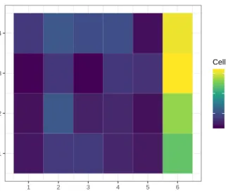
There are two additional visualizations that provide insight into the quality of each cell:mse_heatmap()

andcell_heatmap(). mse_heatmap()gives the mean squared error (MSE) of each cell. Here, MSE

is defined as the mean squared difference between data values and the mean in each cell. Whereas

cell_heatmap()provides a heatmap with the total number of observations in the given cell. Combined, these tools provide valuable insight into the homogeneity of each cell.

(11)

> mse_heatmap(bc) +

+ theme_bw() +

+ scale_fill_viridis_c() +

+ labs(fill = "Cell MSE") +

+ scale_x_continuous(breaks = 1:6) 1 2 3 4 1 2 3 4 5 6

Column Cluster Index

Ro w Cluster Inde x 100 200 300 Cell MSE

Figure 8:A heat map of cell MSEs for the flights biclustering

> cell_heatmap(bc) + + theme_bw() + + scale_fill_viridis_c() 1 2 3 4 1 2 3 4 5 6

Column Cluster Index

Ro w Cluster Inde x 30 60 90 Cell Size

Figure 9:A heat map of cell sizes for the flights biclustering

Finally, for interpretation purposes, retrieving row or column names and their corresponding clusters is easily done using thebiclustermdmethod ofrow.names()(for rows) and use of a new genericcol.names()and its methodcol.names.biclustermd()(for columns). Two final examples are given below showing the output of each function, which have classdata.frame.

> row.names(bc) %>% head() row_cluster name 1 1 January 2 1 April 3 2 February 4 2 March 5 2 August 6 3 May

(12)

> col.names(bc) %>% head() col_cluster name 1 1 ABQ 2 1 ACK 3 1 AUS 4 1 AVL 5 1 BGR 6 1 BQN Further capabilities

As previously mentioned, due to the purposeful randomness of initial row and column clusterings, multiple runs of the algorithm can produce different results. Hence it is recommended to perform several trials (with various parameters) and store the result which obtains the lowest SSE. These multi-ple runs can easily be done in parallel using thetune_biclustermd()function with the parameters as listed below. To utilize this, first a tuning grid must be defined as an input fortune_biclustermd(). Below we provide an illustration of the process.

• data: Dataset to bicluster. Must to be a data matrix with only numbers and missing values in the data set. It should have row names and column names.

• nrep: dataset to bicluster. The number of times to repeat the biclustering for each set of parameters. Default 10.

• parallel: Logical indicating if the user would like to utilize theforeachparallel backend. Default is FALSE.

• ncores: The number of cores to use if parallel computing. Default 2.

• tune_grid: A data frame of parameters to tune over. The column names of this must match the arguments passed tobiclustermd().

> flights_grid <- expand.grid(

+ row_clusters = 4,

+ col_clusters = c(6, 9, 12),

+ miss_val = fivenum(flights),

+ similarity = c("Rand", "Jaccard") + ) > flights_tune <- tune_biclustermd( + flights, + nrep = 10, + parallel = TRUE, + tune_grid = flights_grid + )

The output oftune_biclustermd()is a list of class “biclustermd” and “list” containing the following: • best_combn: The best combination of parameters

• best_bc: The minimum SSE biclustering using the parameters inbest_combn

• grid:tune_gridwith columns giving the minimum, mean, and standard deviation of the final SSE for each parameter combination

• runtime: CPU runtime & elapsed time.

Users can easily identify which set of tuning parameters gives the best results and corresponding performance with the below code. The minimum SSE is obtained when 12 column clusters are used, the missing value used is−34, and the Rand similarity is used. A minimum SSE of 70,698 was obtained in the 10 repeats with that combination, which is a 16% reduction in SSE from our original parameter guesses above. Due to the unsupervised nature of biclustering, ultimately, it is the user’s responsibility to choose reasonable number of row and column clusters for interpretations. Each domain and application of biclustering may lead to a different number of desired row or column clusters for a given array size. We simply utilize the SSE and convergence criteria as quantitative measures in determining the quality of the biclustering result.

> flights_tune$grid[trimws(flights_tune$grid$best_combn) == '*',]

row_clusters col_clusters miss_val similarity min_sse mean_sse sd_sse best_combn

(13)

Any of the previously discussed exploratory functions can be used on the biclustering fit with the best tuning parameters by accessing thebest_bcelement offlights_tunesince it is a biclustermd object:

> flights_tune$best_bc

Initial SSE = 184165; Final SSE = 69586

Rand similarity used; Indices: Columns (P) = 1, Rows (Q) = 1

Finally,biclustermdalso possesses a method forgather()(Wickham and Henry,2019) which provides the name of the row and column a data point comes from as well as its corresponding row and column group association. This is particularly useful since we can easily determine the cell membership of each row and column to do further analysis. Namely, given these associations one can further analyze the quality of each cell and paired with domain knowledge of their data make informed judgments about the value of the biclustering. The following output was created from

flights_tune$best_bc.

> gather(flights_tune$best_bc) %>% head()

row_name col_name row_cluster col_cluster bicluster_no value

1 January ABQ 1 1 1 NA 2 March ABQ 1 1 1 NA 3 April ABQ 1 1 1 12.22222 4 January ACK 1 1 1 NA 5 March ACK 1 1 1 NA 6 April ACK 1 1 1 NA

Example with soybean yield data

For our next example, we perform biclustering on a dataset which has a larger fraction of missing data to further show the practicability of our algorithm. Using data from a commercial soybean breeding program, we consider 132 soybean varieties as rows, 73 locations as columns, and yield in bushels per acre as the response. The locations span across the Midwestern United States and includes parts of Illinois, Iowa, Minnesota, Nebraska, and South Dakota, and each of the 132 soybean varieties represent a different genetic make-up. As one can imagine, not every soybean is grown in each location, as such we obtain a dataset with approximately 72.9% missing values. One application of a dataset such as this would be to determine if there are some subset of soybeans that perform consistently better (or worse) in some locations than others. From a plant breeding perspective, it is of vital importance to understand the relationship between the genetics and environments of crops, and identifying cells non-overlapping homogeneous cells from biclustering can provide insights into this matter (Malosetti et al.,2013).

The main purpose of this dataset is to demonstrate our algorithm on a dataset with a large amount of missing values as well as show the usefulness of the tuning parameters. Below is our first trial on the soybean yield data where we partition into 10 column clusters, 11 row clusters, and use the Jaccard similarity measure. > yield_bc <- biclustermd( + yield, + col_clusters = 10, + row_clusters = 11, + similarity = "Jaccard",

+ miss_val_sd = sd(yield, na.rm = TRUE),

+ col_min_num = 3,

+ row_min_num = 3

+ ) > yield_bc

Initial SSE = 239166; Final SSE = 51813, a 78.3% reduction Jaccard similarity used; Indices: Columns (P) = 1, Rows (Q) = 1

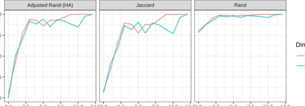
In observing Figure10, we notice that perfect convergence through the Rand Index, adjusted Rand Index, and Jaccard similarity; however, the similarities suggest that the columns converge more

(14)

quickly than the rows. This may be attributed to the high percentage of missing values in the rows of the data table. That is, for each location there is more data available than there is for each soybean variety. Again we notice decreases in the values for each of the three indices, but observing Figure

11, we are assured that the algorithm is only making a column/row swap because a lower SSE is obtainable.

> autoplot(yield_bc$Similarities, facet = TRUE, ncol = 3, size = 0) +

+ theme_bw() + + theme(aspect.ratio = 1) ● ● ● ● ● ● ● ● ● ● ● ● ● ● ● ● ● ● ● ● ● ● ● ● ● ● ● ● ● ● ● ● ● ● ● ● ● ● ● ● ● ● ● ● ● ● ● ● ● ● ● ● ● ● ● ● ● ● ● ● ● ● ● ● ● ● ● ● ● ● ● ● ● ● ● ● ● ●

Adjusted Rand (HA) Jaccard Rand

0.0 2.5 5.0 7.5 10.0 12.50.0 2.5 5.0 7.5 10.0 12.50.0 2.5 5.0 7.5 10.0 12.5 0.00 0.25 0.50 0.75 1.00 Iteration v alue Dimension ● ● Column Row

Figure 10:Plot of similarity measures for the soybean yield biclustering

> autoplot(yield_bc$SSE, size = 1) + + theme_bw() + + theme(aspect.ratio = 1) + + scale_y_continuous(labels = comma) ● ● ● ● ● ● ● ● ● ● ● ● ● 60,000 70,000 80,000 0.0 2.5 5.0 7.5 10.0 12.5 Iteration SSE

Figure 11:SSE plot of soybean yield biclustering

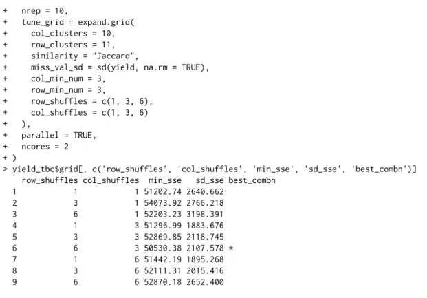
For the initial trial we observe that the Jaccard index converges in 13 iterations to an SSE value of 51,813. To see if it is possible to decrease this SSE even further, we test the impact ofcol_shufflesand

row_shuffles. Recall that these parameters determine how many row and column rearrangements

the algorithm makes before completingoneiteration. Below we usetune_biclustermd() to test combinations ofcol_shufflesandrow_shufflesas well as its corresponding SSE. We define the tune grid to mimic that of theyield_bccreation above, but letcol_shufflesandrow_shufflestake on values in{1, 3, 6}independent of each other. We repeat the biclustering ten times for each parameter, specified bynrep = 10. Note thatparallel = TRUEallows us to tune over the grid in parallel.

> yield_tbc <- tune_biclustermd(

(15)

+ nrep = 10,

+ tune_grid = expand.grid(

+ col_clusters = 10,

+ row_clusters = 11,

+ similarity = "Jaccard",

+ miss_val_sd = sd(yield, na.rm = TRUE),

+ col_min_num = 3, + row_min_num = 3, + row_shuffles = c(1, 3, 6), + col_shuffles = c(1, 3, 6) + ), + parallel = TRUE, + ncores = 2 + )

> yield_tbc$grid[, c('row_shuffles', 'col_shuffles', 'min_sse', 'sd_sse', 'best_combn')]

row_shuffles col_shuffles min_sse sd_sse best_combn

1 1 1 51202.74 2640.662 2 3 1 54073.92 2766.218 3 6 1 52203.23 3198.391 4 1 3 51296.99 1883.676 5 3 3 52869.85 2118.745 6 6 3 50530.38 2107.578 * 7 1 6 51442.19 1895.268 8 3 6 52111.31 2015.416 9 6 6 52870.18 2652.400

Algorithm time study with movie ratings data

For our last example, we focus our attention on a movie ratings dataset obtained from MovieLens (Harper and Konstan,2015). If we consider movie raters as defining rows, movies as defining columns, and a rating from 1–5 (with 5 being the most favorable) as a response, then biclustering can be used to determine subsets of raters who have similar preferences towards some subset of movies.

The main topic of this section will be to perform time studies to test the scalability of our proposed algorithm. In some applications, it is not uncommon to have a two-way data table with 10,000+ rows or columns. Intuitively as the dimensions of the two-way data table increases so will the computational time. In it is not uncommon for other biclustering algorithms to run for 24+ hours (?). We ran the biclustering over a grid of 80 combinations ofIrows,Jcolumns,rrow clusters, andccolumn clusters with 30 replications for each combination. In addition to the four grid parameters, we consider the following metrics which are byproducts of the four parameters: the size of the datasetN = I×J, average row cluster sizeI/r, and average column cluster size J/c. Table1summarizes the grid parameters, their byproducts and the defined lower and upper limits on each.

N

=

I

×

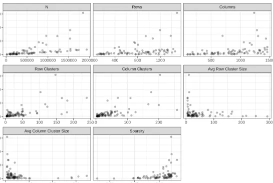
J I J r c I/r J/c Lower Limit 2,500 50 50 4 4 5 5 Min 18,146 86 98 4 4 5 5 Mean 665,842 784 839 42 45 49 47 Max 1,929,708 1,495 1,457 239 258 293 346 Upper Limit 2,225,000 1,500 1,500 300 300 375 375

Table 1:Summary of the movie data runtime grid with defined lower and upper limits Table2gives a five number summary and the mean runtime in seconds paired with the parameters which produced run times closest to each statistic. In all, we see that the algorithm can take less than a second to run, while in the other extreme the algorithm requires 39 minutes to converge. It is particularly interesting that for the two parameter combinations closest to the median run time, one dataset is nearly twice the size of the other. Furthermore, note than the mean run time is more than twice that of the median, but the size of the dataset is just 38% of that at the median. However, at the mean, 3744=72·52 biclusters are computed, while at the medians, only 80=20·4 and 481=13·37 biclusters are computed. For a visual summary of the results, we point the reader to Figure12.

Figure12plots run times versus the five parameters controlled for in the study as well as average row cluster size, average column cluster size, and sparsity. We encourage the reader to personally

(16)

Seconds I J N r c Sparsity Min 0.4 210 98 20,580 10 9 96.2% Q1 24.7 820 184 150,880 53 12 98.2% Median 63.6 988 1,240 1,225,120 20 4 98.5% Median 63.5 501 1,302 652,302 13 37 98.0% Mean 137.5 1,084 427 462,868 72 52 98.4% Q3 141.0 485 875 424,375 36 126 98.0% Max 2,369.0 1,495 1,233 1,843,335 147 204 98.5%

Table 2:Five number summary and mean runtime in seconds along with parameters achieved at

explore the results; the run time data is theruntimesdataset in the package. Moreover,Li et al.(2020), provides further insights into the effect of sparsity on runtimes.

Avg Column Cluster Size Sparsity

Row Clusters Column Clusters Avg Row Cluster Size

N Rows Columns 0 100 200 300 0.96 0.97 0.98 0 50 100 150 200 250 0 100 200 0 100 200 300 0 500000 1000000 1500000 2000000 400 800 1200 500 1000 1500 0 500 1,000 1,500 0 500 1,000 1,500 0 500 1,000 1,500 value A v er

age Time (sec)

Figure 12:Relationship between movie grid parameters and elapsed time

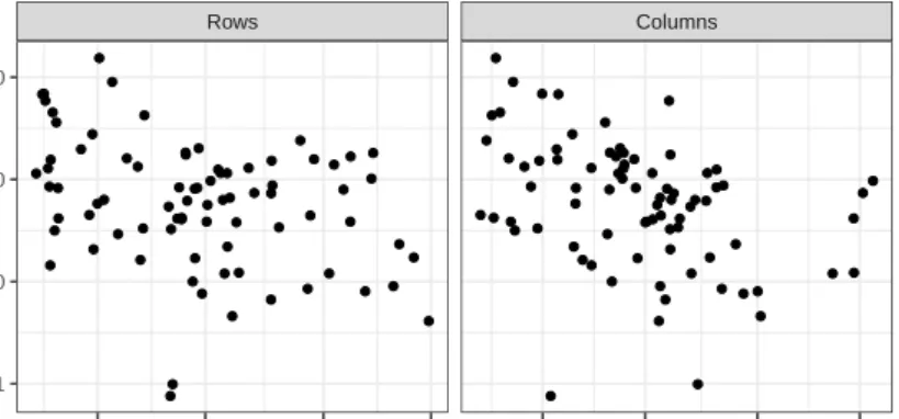
Finally, we address the trade-off between interpretability and computation time. Figure13plots elapsed time versus average cluster size on a doubly log 10 scales for row clusters (left) and column clusters (right). Clearly, computation time can be decreased by increasing the average cluster size, but doing so potentially reduces the interpretability of results; biclusters may be too large for certain use cases. Keeping in mind that they-axis is on a log 10 scale, increasing average cluster size will have diminishing returns. Reviewing the plot on the right-hand side of the second row and the left-hand side of row three in Figure12sheds more light into this notion.

Summary

Based on the work of (Li et al.,2020) we provide a user-friendly R implementation of their proposed biclustering algorithm for missing data as well as a variety of visual aids that are helpful for biclustering in general and biclustering with missing data specifically. The unique benefitbiclustermdprovides is in its ability to operate with missing values. Compared to other packages which do not allow incomplete data or make use of some sort of imputation, we approach this problem with a novel framework that does not alter the structure of an inputted data matrix. Moreover, given the tunability of our biclustering algorithm, users are able to run trials on numerous combinations in an attempt to best bicluster their data.

(17)

● ●●_● ● ● ● ● ● ● ● ● ● ● ● ● ● ● ● ● ● ● ● ● ● ● ● ● ● ● ● ● ● ● ● ● ● ● ● ● ● ● ● ● ● ● ●●● ● ● ● ● ● ● ● ● ● ● ● ● ● ● ● ● ● ● ● ● ● ● ● ● ● ● ● ● ● ● ● ● ● ● _● ● ● ● ● ● ● ● ● ● ● ● ● ● ● ● ● ● ● ● ● ● ● ● ● ● ● ● ● ● ● ● ● ● ● ● ● ● ● ● ● ● ● ● ● ● ● ● ● ● ● ● ● ● ● ● ● ● ● ● ● ● ● ● ● ● ● ● ● ● ● ● ● ● ● ● ● Rows Columns 10 30 100 300 10 30 100 300 1 10 100 1,000

Average Cluster Size

A

v

er

age Time (sec)

Figure 13:Relationship between average cluster sizes and elapsed time

Acknowledgments

This research was supported in part by Syngenta Seeds and by a Kingland Data Analytics Faculty Fellowship at Iowa State University.

Bibliography

S. Bergmann, J. Ihmels, and N. Barkai. Iterative Signature Algorithm for the Analysis of Large-Scale Gene Expression Data. Physical Review E - Statistical Physics, Plasmas, Fluids, and Related Interdisciplinary Topics, 2003. ISSN 1063651X. URLhttps://doi.org/10.1103/PhysRevE.67.031902. [p1]

S. Busygin, O. Prokopyev, and P. M. Pardalos. Biclustering in Data Mining.Computers and Operations Research, 35(9), 2008. URLhttps://doi.org/10.1016/j.cor.2007.01.005. [p1]

Y. Cheng and G. M. Church. Biclustering of Expression Data. Proceedings International Conference on Intelligent Systems for Molecular Biology ; ISMB. International Conference on Intelligent Systems for Molecular Biology, 8, 2000. [p1]

D. T. Ewoud.BiBitR: R Wrapper for Java Implementation of BiBit, 2017. R package version 0.4.2. [p1] D. W. Goodall. A new similarity index based on probability.Biometrics, 22:882–907, 1966. [p3] D. Gusenleitner and A. Culhane. iBBiG: Iterative Binary Biclustering of Genesets, 2019. URLhttp:

//bcb.dfci.harvard.edu/~aedin/publications/. R package version 1.28.0. [p1]

F. M. Harper and J. A. Konstan. The MovieLens Datasets.ACM Transactions on Interactive Intelligent Systems, 2015. [p13]

J. A. Hartigan. Direct Clustering of a Data Matrix.Journal of the American Statistical Association, 67(337): 123–129, 1972. URLhttps://doi.org/10.1080/01621459.1972.10481214. [p1]

L. Hubert and P. Arabie. Comparing Partitions.Journal of Classification, 1985. ISSN 01764268. URL

https://doi.org/10.1007/bf01908075. [p3]

S. Kaiser and F. Leisch. A Toolbox for Bicluster Analysis in {R}. Compstat 2008—Proceedings in Computational Statistics, pages 201–208, 2008. [p1]

T. Khamiakova. Superbiclust: Generating Robust Biclusters from a Bicluster Set (Ensemble Biclustering), 2014. URLhttps://CRAN.R-project.org/package=superbiclust. R package version 1.1. [p1] Y. Kluger, R. Basri, J. T. Chang, and M. Gerstein. Spectral Biclustering of Microarray Data: Coclustering

Genes and Conditions.Genome Research, 13(4):703–716, 2003. URLhttps://doi.org/10.1101/gr.

648603. [p1]

L. Lazzeroni and A. Owen. Plaid Models for Gene Expression Data.Statistica Sinica, 12:61–86, 2002. ISSN 10170405. URLhttps://doi.org/10.1017/CBO9781107415324.004. [p1]

J. Li, J. Reisner, H. Pham, S. Olafsson, and S. Vardeman. Biclustering for Missing Data. Information Sciences, 510:304–316, 2020. URLhttps://doi.org/10.1016/j.ins.2019.09.047. [p2,5,14]

(18)

M. Malosetti, J. M. Ribaut, and F. A. van Eeuwijk. The Statistical Analysis of Multi-Environment Data: Modeling Genotype-by-Environment Interaction and Its Genetic Basis.Frontiers in Physiology, 4(44), 2013. URLhttps://doi.org/10.3389/fphys.2013.00044. [p11]

M. Rand. Objective Criteria for the Evaluation of Methods Clustering.Journal of the American Statistical Association, 66(336):846–850, 1971. URLhttps://doi.org/10.1080/01621459.1971.10482356. [p3] M. Sill and S. Kaiser.S4vd: Biclustering via Sparse Singular Value Decomposition Incorporating Stability Selection, 2015. URLhttps://CRAN.R-project.org/package=s4vd. R package version 1.1-1. [p1] K. M. Tan and D. M. Witten. Sparse Biclustering of Transposable Data.Journal of Computational and

Graphical Statistics, 2014. ISSN 15372715. URLhttps://doi.org/10.1080/10618600.2013.852554. [p1]

H. Wickham.Ggplot2: Elegant Graphics for Data Analysis. Springer-Verlag, 2009. ISBN 978-0-387-98140-6. URLhttp://ggplot2.org. [p5]

H. Wickham. Nycflights13: Flights That Departed NYC in 2013, 2017. URLhttps://CRAN.R-project.

org/package=nycflights13. R package version 0.2.2. [p4]

H. Wickham and L. Henry.Tidyr: Easily Tidy Data with ’Spread()’ and ’Gather()’ Functions, 2019. URL

https://CRAN.R-project.org/package=tidyr. R package version 0.8.3. [p11]

Y. Zhang, J. Xie, J. Yang, A. Fennell, C. Zhang, and Q. Ma. QUBIC: a bioconductor package for qualitative biclustering analysis of gene co-expression data.Bioinformatics, 33(3):450–452, 2017. URL

https://doi.org/10.1093/bioinformatics/btw635. [p1] John Reisner

Department of Statistics Iowa State University United States

[email protected]

Hieu Pham

Department of Industrial and Manufacturing Systems Engineering Iowa State University

United States

[email protected]

Sigurdur Olafsson

United States

[email protected]

Stephen Vardeman Department of Statistics

United States