SORT 38 (2) July-December 2014, 161-180 c Institut d’Estad´ıstica de CatalunyaOperations ResearchTransactions [email protected] ISSN: 1696-2281
eISSN: 2013-8830 www.idescat.cat/sort/
Estimators for the parameter mean of
Morgenstern type bivariate generalized
exponential distribution using ranked set sampling
Saeid Tahmasebi1and Ali Akbar Jafari2Abstract
In situations where the sampling units in a study can be more easily ranked based on the measurement of an auxiliary variable, ranked set sampling provides unbiased estimators for the mean of a population that are more efficient than unbiased estimators based on simple random sampling. In this paper, we consider the Morgenstern type bivariate generalized exponential distribution and obtain several unbiased estimators for the mean parameter of its marginal distribution, based on different ranked set sampling schemes. The efficiency of all considered estimators are evaluated and several numerical illustrations are given.
MSC: 62D05; 62F07;62G30.
Keywords: Concomitants of order statistics, Morgenstern type bivariate generalized exponential distribution, ranked set sampling.
1. Introduction
Ranked set sampling (RSS) was first suggested by McIntyre (1952) for estimating mean pasture and forage yields. RSS is applicable whenever ranking of a set of sampling units can be done easily by a judgement method with respect to the variable of interest. Later, Takahasi and Wakimoto (1968) provided the statistical foundation and necessary math-ematical properties of the method. They indicated that in situations where the sampling units in a study can be more easily ranked based on the measurement of an auxiliary
∗Corresponding author e-mail: [email protected]
1Department of Statistics, Persian Gulf University, Bushehr, Iran. 2Department of Statistics, Yazd University, Yazd, Iran.
Received: August 2013 Accepted: May 2014
variable, RSS provides unbiased estimators for the mean of a population, and these estimators are more efficient than unbiased estimators based on simple random sampling (SRS).
The RSS technique is composed of two stages in a sample selection procedure: At
the first stage,nsimple random samples of sizenare drawn from a population and each
sample is called a set. Then, each of the units are ranked from the smallest to the largest
according to a variable of interest, sayY, in each set based on a low-level measurement
such as a concomitant variable or previous experience. At the second stage, the first unit
from the first set, the second unit from the second set and going on like this till thenth
unit from thenth set are taken and measured according to the variableY. The obtained
sample is called a RSS. It can be noted that the units of this sample are independent order statistics but not identically distributed. The reader can refer to the book of Chen et al. (2004) for details of RSS and its applications.
Other schemes and modifications of RSS were investigated in the literature: A mod-ified RSS procedure is introduced by Stokes (1980) and only the largest or the smallest judgment ranked unit is chosen for quantification in each set. In estimating the popu-lation mean, Samawi et al. (1996) suggested the extreme ranked set sampling (ERSS), Muttlak (1997) suggested the median RSS, Jemain and Al-Omari (2006) suggested dou-ble quartile ranked set samples, and Al-Odat and Al-Saleh (2001) suggested moving extreme ranked set sampling (MERSS). Yu and Tam (2002) considered the problem of estimating the mean of a population based on RSS with censored data. Al-Saleh and Al-Kadiri (2000) considered double RSS (DRSS), and Al-Saleh and Al-Omari (2002) generalized the DRSS to the multistage ranked set sampling (MSRSS) method. For the mean normal or exponential, Sinha et al. (1996) used median ranked set sampling (MRSS) to modify the RSS estimators Muttlak (2003) introduced percentile ranked set sampling (PRSS). Al-Nasser (2007) proposed a generalized robust sampling method called L ranked set sampling (LRSS) and showed that the estimator for the mean based on the LRSS is unbiased if the underlying distribution is symmetric. A robust extreme ranked set sampling (RERSS) is proposed by Al-Nasser and Mustafa (2009) for esti-mating the population mean.
RSS and its modifications are applied for estimating a parameter in a bivariate
population(X,Y), whereY is the variable of interest and X is a concomitant variable
that is not of direct interest but is relatively easy to measure or to order by judgment: Stokes (1977) studied RSS with concomitant variables. Barnett and Moore (1997)
derived the best linear unbiased estimator (BLUE) for the mean of Y, based on a
ranked set sample obtained using an auxiliary variableX. Al-Saleh and Al-Ananbeh
(2007) estimated the means of the bivariate normal distribution using moving extremes RSS. Chacko and Thomas (2008) and Al-Saleh and Diab (2009) considered estimation of a parameter of Morgenstern type bivariate exponential distribution and Downton’s bivariate exponential distribution, respectively. Tahmasebi and Jafari (2012) assumed the Morgenstern type bivariate uniform distribution and obtained several estimators for a scale parameter.
The distribution function of a Morgenstern type bivariate generalized exponential distribution (MTBGED) is defined as
FX,Y(x,y) = (1−e−θ1x)α1(1−e−θ2y)α2[1+λ(1−(1−e−θ1x)α1)(1−(1−e−θ2y)α2)], (1)
x,y>0,−1≤λ≤1,α1,α2,θ1,θ2>0,
with the corresponding probability density function (pdf)
fX,Y(x,y) = α1α2θ1θ2e−θ1x−θ2y(1−e−θ1x)α1−1(1−e−θ2y)α2−1
×n1+λ[2(1−e−θ1x)α1−1][2(1−e−θ2y)α2−1]
o
. (2)
Note that when (X,Y) has MTBGED, the marginal distribution ofX andY is the
generalized exponential distribution with the expected values
µx= B(α1) θ1 , µy= B(α2) θ2 ,
respectively, whereB(α) =ψ(α+1)−ψ(1)andψ(.)is the digamma function. Also,
the correlation coefficient betweenX andY is obtained as (see Tahmasebi and Jafari,
2013)
ρ= pλD(α1)D(α2)
C(α1)C(α2) =λg(α1)g(α2), (3)
whereD(α) =B(2α)−B(α),C(α) =ψ′(1)−ψ′(α+1),ψ′(.)is the derivative of the digamma function, andg(α) =√D(α)
C(α).
In this paper, we consider estimation of the parameterµy whenα2 is known, and
propose several estimator based on the RSS idea. Also, we suggest some improved version of these estimators. In Section 2, we present unbiased estimators for the
parameter µy in MTBGED based on the RSS, LRSS, ERSS, MERSS, and MSRSS
methods. We evaluate the efficiency of all considered estimators in Section 3.
2. Unbiased estimators for
µµµyyybased on different RSS schemes
Suppose that the random variable (X,Y) has a MTBGED as defined in (1). In this
section, we find unbiased estimators for the parameterµy based on different sampling
schemes. In each case, first the general pattern of sampling is presented, and then an
unbiased estimator with its variance is given for the parameterµy. Also, the efficiency
2.1. RSS estimation
The procedure of RSS is described by Stokes (1977) for a bivariate random variable by the following steps:
Step 1. Randomly selectnindependent bivariate samples, each of sizen.
Step 2. Rank the units within each sample with respect to variableX together with the
Y variate associated.
Step 3. In the rth sample of size n, select the unit (X(r)r,Y[r]r), r =1,2, . . . ,n, where
X(r)r is the measured observation on the variableX in therth unit andY[r]r is the
corresponding measurement made on the study variableY of the same unit.
Therefore,Y[r]r, r =1,2,3, . . . ,n, are the RSS observations made on the units of the
RSS regarding the study variableY which is correlated with the auxiliary variableX.
Therefore, clearlyY[r]r is the concomitant of rth order statistic arising from the rth sample.
From Scaria and Nair (1999) the pdf ofY[r]rfor 1≤r≤nis given by
h[r]r(y) =α2θ2e−θ2y(1−e−θ2y)α2−1[1+δr(1−2(1−e−θ2y)α2)], 1≤r≤n, (4)
whereδr=λ(
n−2r+1)
n+1 and its mean and variance ofY[r]rare obtained by Tahmasebi and
Jafari (2013) as E[Y[r]r] = 1 θ2 [B(α2)−δrD(α2)], Var[Y[r]r] = 1 θ2 2 [C(α2) +δr(C(2α2)−C(α2))]. (5)
SinceY[r]randY[s]sforr6=sare drawn from two independent samples, so we have
Cov(Y[r]r,Y[s]s) =0, r6=s.
Theorem 1 Based on the RSS procedure, an unbiased estimator forµyis given by
ˆ µRSS= 1 n n
∑
r=1 Y[r]r,and its variance is
Var(µˆRSS) =
C(α2)
nθ2 2
Proof.Since∑nr=1δr=∑nr=1 λ(n−2r+1) n+1 =0, using (5) E(µˆRSS) = 1 n n
∑
r=1 E Y[r]r = 1 nθ2 n∑
r=1 (B(α2)−δrD(α2)) = B(α2) θ2 =µy, and Var(µˆRSS) = 1 n n∑
r=1 Var Y[r]r = 1 n2θ2 2 n∑
r=1 [C(α2) +δr(C(2α2)−C(α2))] = 1 n2θ2 2 n∑
r=1 [C(α2) +δr(C(2α2)−C(α2))] = C(α2) nθ2 2 .Now, we study the efficiency of ˆµRSSrelative to the BLUE ofµy, ˜µ, based onY[r]r,
r=1,2,3, . . . ,n, for MTBGED, whenλis known. From David and Nagaraja (2003, p.
185) the BLUE ofµyis derived as
˜ µ= n
∑
r=1 arY[r]r, where ar= H(α2,r) W(α2,r) ( n∑
j=1 [H(α2,j)]2 W(α2,j) )−1, r=1,2,3, . . . ,n,H(α2,r) =1−δBrD(α(α2)2) andW(α2,r) =C(α2) +δr[C(2α2)−C(α2)]. The variance of ˜µ is Var[µ˜] = v2 θ2 2 , wherev2= n ∑ r=1 [H(α2,r)]2 W(α2,r) −1
, and therefore, the relative efficiency of ˆµRSSto ˜µis given by e1=e(µ˜ |µˆRSS) = C(α2) n n
∑
r=1 [H(α2,r)]2 W(α2,r) .In Section 3, we calculate the relative efficiency of ˆµRSSto ˜µ,e1, for some values of the parameters and sample size.
Remark 2 We know that the correlation coefficient between X and Y in MTBGED is
λg(α1)g(α2). So whenα1andα2are known, by using the sample correlation coefficient q of the RSS observations(X(r)r,Y[r]r), r=1,2,3, . . . ,n an estimator forλis given by
ˆ λ= −1 q<−g(α1)g(α2) q g(α1)g(α2) −g(α1)g(α2)≤q≤g(α1)g(α2) 1 g(α1)g(α2)<q
Sometimes, k units of observations are censored in the RSS schemes. LetY[mr]mr,
r=1,2, . . . ,n−k, be the ranked set sample observations on the study variableY, which
results from censoring and ranking on the auxiliary variableX. We can represent the
ranked set sample observations on the study variateY as p1Y[1]1, p2Y[2]2, . . . ,pnY[n]n,
where pr=0 if the rth unit is censored, and pr=1 otherwise. Consider k units are
censored. Hence∑nr=1pr=n−k. if we writemr,r=1,2, . . . ,n−k, as the integers such that 1≤m1<m2<···<mn−k≤nandpmr=1, then
E ∑nr=1prY[r]r n−k = 1 θ2 B(α2)−D(α2) n−k n−k
∑
r=1 δmr ! ,Therefore, the ranked set sample mean in the censored case is not an unbiased estimator forµy. However, we can construct an unbiased estimator based on this expected value.
Theorem 3 An unbiased estimator forµybased on the censored RSS is given by
ˆ µCRSS= 1 w n−k
∑
r=1 Y[mr]mr, where w=n−k+1−B(2α2) B(α2)∑nr=−1kδmr, and its variance is
Var(µˆCRSS) = v3 θ2 2 , where v3=w12∑ n−k r=1[C(α2) +δmr(C(2α2)−C(α2))]. Proof E(µˆCRSS) = 1 w n−k
∑
r=1 E(Y[mr]mr) = ∑nr=−1k(B(α2)−δmrD(α2)) (n−k−D(α2) B(α2)∑ n−k r=1δmr)θ2 =B(α2) θ2 =µy,2.2. LRSS estimation
Al-Nasser (2007) proposed a generalized robust sampling method called L ranked set sampling (LRSS) for estimating population mean. The procedure of LRSS with a concomitant variable is as follows:
Step 1. Randomly selectnindependent bivariate samples, each of sizen.
Step 2. Rank the units within each sample with respect to variableX together with the
Y variate associated.
Step 3. Select the LRSS coefficient, k= [nγ], such that 0≤γ< .5, where[x] is the largest integer value less than or equal tox.
Step 4. For each of the firstk+1 ranked samples of sizen, select the unit(X(k+1)r,Y[k+1]r),
r=1,2, . . . ,k.
Step 5. For each of the lastk+1 ranked samples of sizen, i.e., the(n−k)th to thenth ranked sample, select the unit(X(n−k)r,Y[n−k]r),r=n−k+1, . . . ,n.
Step 6. For j=k+2, . . . ,n−k−1, select the unit(X(r)r,Y[r]r),r=k+1, . . . ,n−k.
Note that this LRSS scheme leads to the RSS when k=0, and to the traditional
MRSS whenk=n−1
2
. Also, the PRSS could be considered as a special case of this scheme.
Theorem 4 An unbiased estimator ofµy in MTBGED based on LRSS scheme is given
by ˆ µLRSS= 1 n k
∑
r=1 Y[k+1]r+ n−k∑
r=k+1 Y[r]r+ n∑
r=n−k+1 Y[n−k]r ! , with variance Var(µˆLRSS) =Var(µˆRSS) = C(α2) nθ2 2 . (7) Proof.Since k∑
r=1 δk+1= λ n+1 k∑
r=1 (n−2(k+1) +1) = λk n+1(n−2k−1), k∑
r=1 δn−k= λ n+1 n∑
r=n−k+1 (n−2(n−k) +1) = λk n+1(−n+2k+1), n−k∑
r=k+1 δr= λ n+1 n−k∑
r=k+1 (n−2r+1) =0,we have E(µˆLRSS) = 1 n kB(α2) θ2 − D(α2) θ2 λk n+1(n−2k−1) + kB(α2) θ2 −D(θα2) 2 λk n+1(−n+2k+1) + (n−2k)B(α2) θ2 = B(α2) θ2 =µy, and Var(µˆLRSS) = 1 n2 kC(α2) θ2 2 −C(2α2)θ−C(α2) 2 λk n+1(n−2k−1) + kC(α2) θ2 2 −C(2α2)θ−2C(α2) 2 λk n+1(−n+2k+1) + (n−2k)C(α2) θ2 2 =C(α2) nθ2 2 . 2.3. ERSS estimation
The extreme ranked set sampling (ERSS) method with concomitant variable, introduced by Samawi et al. (1996), can be described as follows:
Step 1. Selectnrandom samples each of sizenbivariate units from the population.
Step 2. If the sample sizenis even, then select fromn2samples the smallest ranked unit
X together with the associatedY and from the other n2 samples the largest ranked
unitX together with the associatedY. These selected observations (X(1)1,Y[1]1), (X(n)2,Y[n]2),(X(1)3, Y[1]3), . . . ,(X(1)n−1,Y[1]n−1),(X(n)n,Y[n]n) can be denoted by ERSS1.
Step 3. If n is odd then select from n−21 samples the smallest ranked unitX together with the associatedY and from the other n−21samples the largest ranked unitX
to-gether with the associatedY and from one sample the median of the sample for
ac-tual measurement. In this case the selected observations(X(1)1,Y[1]1),(X(n)2,Y[n]2), (X(1)3,Y[1]3), . . . ,(X(n)n−1,Y[n]n−1),(
X(1)n+X(n)n
2 ,
Y[1]n+Y[n]n
2 )can be denoted ERSS2and
(X(1)1,Y[1]1),(X(n)2,Y[n]2),(X(1)3,Y[1]3), . . . ,(X(n)n−1,Y[n]n−1),(X(n+1
2 )n,Y[n+21]n)can be
denoted by ERSS3.
Theorem 5 (i) if n is even, then an unbiased estimator forµyusing ERSS1is defined as
ˆ µERSS1= 1 n n/2
∑
r=1 (Y[1]2r−1+Y[n]2r),with variance
Var(µˆERSS1) =Var(µˆRSS) =
C(α2)
nθ2 2
.
(ii) If n is odd then unbiased estimators forµyusing ERSS2and ERSS3are obtained as
ˆ µERSS2= 1 n (n−1)/2
∑
r=1 (Y[1]2r−1+Y[n]2r) + Y[1]n+Y[n]n 2n , ˆ µERSS3= 1 n (n−1)/2∑
r=1 (Y[1]2r−1+Y[n]2r) + Y[n+1 2 ]n n , with variance Var(µˆERSS2) = v4 θ2 2 , (8)Var(µˆERSS3) =Var(µˆERSS1) =
C(α2) nθ2 2 , (9) respectively, where v4=21n2{(2n−1)C(α2) + 4λ 2D2(α 2) (n+1)2(n+2)}.
Proof.(i) Since
n/2
∑
r=1 δ1= λn(n−1) 2(n+1) , n/2∑
r=1 δn= λn(−n+1) 2(n+1) , we have E(µˆERSS1) = 1 n( nB(α2) 2θ2 − D(α2) θ2 λn(n−1) 2(n+1) + nB(α2) 2θ2 − D(α2) θ2 λn(−n+1) 2(n+1) ) = B(α2) θ2 , Var(µˆERSS1) = 1 n2( nC(α2) 2θ2 2 +C(2α2)−C(α2) θ2 2 λn(n−1) 2(n+1) + nC(α2) 2θ2 2 +C(2α2)−C(α2) θ2 2 λn(−n+1) 2(n+1) ) = C(α2) nθ2 2 .(ii) In the estimator ˆµERSS2, it is easy to see thatY[1]1,Y[n]2,Y[1]3, . . . ,Y[n]n−1are indepen-dent ofY[1]nandY[n]n, but the random variablesY[1]nandY[n]nare dependent. From Scaria and Nair (1999) the joint density function of(Y[1]n,Y[n]n)is given by
h[1,n]n(z,w) = (α2θ2)2e−θ2(z+w)[(1−e−θ2z)(1−e−θ2w)] α2−1 {1+2λ(n−1) n+1 [(1−e −θ2w)α2 −(1−e−θ2z)α2] +δ 1,n[1−2(1−e−θ2w) α2 ][1−2(1−e−θ2z)α2]}, whereδ1,n=λ 2(−n2+n+2) (n+1)(n+2) . Therefore, Cov(Y[1]n,Y[n]n) =E[Y[1]nY[n]n]−E[Y[1]n]E[Y[n]n] = D2(α2) θ2 2 [δ1,n−δ1δn] =λ 2D2(α 2) θ2 2 [ −n 2+n+2 (n+1)(n+2)+ ( n−1 n+1) 2] = 4λ2D2(α2) (n+1)2(n+2)θ2 2 . Also,Y[1]1,Y[n]2,Y[1]3, . . . ,Y[n]n−1andY[n+1
2 ]nare all independent in ˆµERSS3. Since
(n−1)/2
∑
r=1 δ1= λ(n−1)2 2(n+1) , (n−1)/2∑
r=1 δn=− λ(n−1)2 2(n+1) , δ(n+1)/2=0, we have E(µˆERSS2) = 1 n (n−1)B(α2) 2θ2 − D(α2) θ2 λ(n−1)2 2(n+1) + (n−1)B(α2) 2θ2 +D(α2) θ2 λ(n−1)2 2(n+1) +B(α2) 2θ2 − D(α2) 2θ2 λ(n−1) (n+1) + B(α2) 2θ2 +D(α2) 2θ2 λ(n−1) (n+1) =B(α2) θ2 , E(µˆERSS3) = 1 n (n−1)B(α2) 2θ2 − D(α2) θ2 λ(n−1)2 2(n+1) + (n−1)B(α2) 2θ2 +D(α2) θ2 λn(n−1)2 2(n+1) + B(α2) θ2 =B(α2) θ2 , Var(µˆERSS2) = 1 n2 (n−1)C(α2) 2θ2 2 +C(2α2)−C(α2) θ2 2 λ(n−1)2 2(n+1) + (n−1)C(α2) 2θ2 2 −C(2α2)θ−2C(α2) 2 λ(n−1)2 2(n+1) + C(α2) 4θ2 2 +C(2α2)−C(α2) 4θ2 2 λ(n−1) 2(n+1) +C(α2) 4θ2 2 −C(2α24)θ−2C(α2) 2 λ(n−1) 2(n+1) + 1 2Cov(Y[1]n,Y[n]n) = 1 2θ2 2n2 (2n−1)C(α2) + 4λ2D2(α 2) (n+1)2(n+2) ,Var(µˆERSS3) = 1 n2 (n−1)C(α2) 2θ2 2 +C(2α2)−C(α2) θ2 2 λ(n−1)2 2(n+1) + (n−1)C(α2) 2θ2 2 −C(2α2)θ−2C(α2) 2 λ(n−1)2 2(n+1) + C(α2) θ2 2 ! =C(α2) nθ2 2 .
By using (6) and (8) the efficiency of ˆµRSSrelative to the estimator ˆµERSS2 is given by e2=e(µˆERSS2|µˆRSS) = 2nC(α2) (2n−1)C(α2) + 4λ 2D2(α 2) (n+1)2(n+2) .
Note thate2decreases with respect to|λ|for fixedn. Also, limn→∞e2=1.In Section 3, we calculate the relative efficiency of ˆµERSS2 to ˆµRSS, e2, for some values of the parameters and sample size.
2.4. MERSS estimation
Al-Odat and Al-Saleh (2001) suggested the MERSS, and Al-Saleh and Al-Ananbeh (2007) used the concept of MERSS with concomitant variable for the estimation of the means of the bivariate normal distribution. The procedure of MERSS with concomitant variable in MTBGED is as follows:
Step 1. Select n units each of size n from the population using SRS. Identify by
judgment the minimum of each set with respect to the variable X together with
the associatedY.
Step 2. Repeat step 1, but for the maximum.
Note that the 2n pairs of set {(X(1)r,Y[1]r),(X(n)r,Y[n]r);r=1,2, . . . ,n} that are ob-tained using the above procedure, are independent but not identically distributed.
Theorem 6 An unbiased estimator forµybased on MERSS is given by
ˆ µMERSS= 1 2n n
∑
r=1 (Y[1]r+Y[n]r),and its variance is
Var(µˆMERSS) = C(α2) 2nθ2 2 = 1 2Var(µˆRSS).
Proof.The proof is similar to proof of Theorem 5, part (i).
2.5. MSRSS estimation
Al-Saleh and Al-Kadiri (2000) have considered DRSS to increase the efficiency of
the RSS estimator without increasing the set size n. Al-Saleh and Al-Omari (2002)
generalized DRSS to MSRSS. The MSRSS scheme can be described as follows:
Step 1. Randomly selectednl+1sample units from the population, wherelis the number of stages, andnis the set size.
Step 2. Allocate thenl+1selected units randomly intonl−1sets, each of sizen2.
Step 3. For each set in Step 2, apply the procedure of ranked set sampling method with
respect to variableX to obtain a (judgment) ranked set, of sizen; this step yields
nl−1(judgment) ranked sets, of sizeneach.
Step 4. Without doing any actual quantification on these ranked sets, repeat Step 3 on thenl−1ranked sets to obtainnl−2second stage (judgment) ranked sets, of sizen each.
Step 5. This process is continued, without any actual quantification, until we end up with thelth stage (judgement) ranked set of sizen.
Step 6. Finally, thenidentified in step 5 are now quantified for the variableX together with the associatedY. Show the value measured for(X,Y)on the units selected at therth stage of the MSRSS by(X((rl))r,Y[r(l])r),r=1, ...n.
For λ>0, letY[(nl])r,r=1,2, . . . ,n, be the value measured on the units selected at
therth stage of the unbalanced MSRSS (Similar to suggestion by Chacko and Thomas,
2008). It is easily to see that eachY[(nl])ris the concomitant of the largest order statistic of
nrindependently and identically distributed bivariate random variables with MTBGED,
and therefore, the pdf ofY[(nl])ris given by
h([nl)]r(y) =α2θ2e−θ2y(1−e−θ2y)α2−1[1+λ(n l
−1)
nl+1 (2(1−e
−θ2y)α2−1)].
Thus the mean and variance ofY[(nl])rforr=1,2, . . . ,n, are given as
E[Y[(nl])r] =µyξnl, Var[Y( l) [n]r] = γnl θ2 2 , (10) respectively, whereξnl =1+λ(n l−1)D(α 2) (nl+1)B(α2) andγnl=C(α2) +λ(n l−1) nl+1 (C(α2)−C(2α2)).
Theorem 7 Ifα2andλare known then the BLUE ofµyis ˆ µMSRSS= 1 nξnl n
∑
r=1 Y[(nl])r, (11) with variance Var(µˆMSRSS) = γnl nξ2 nlθ22 . (12)Proof.It can easily be proved using (10).
If we takel=1 in (11) and (12), then we get the BLUE ofµybased the usual single
stage unbalanced RSS (URSS) as
ˆ µURSS= 1 nξn n
∑
r=1 Y[n]r,where its variance is given as
Var(µˆURSS) =
γn
nξ2 nθ22
. (13)
If we letl→∞in the MSRSS method described above, thenY[n(∞]r),r=1,2, . . . ,nare
unbalanced steady-state ranked set samples (USSRSS) of sizenwith the following pdf
(Al-Saleh, 2004):
h([n∞]r)(y) =α2θ2e−θ2y(1−e−θ2y)α2−1[1+λ(2(1−e−θ2y)α2−1)].
The mean and variance ofY[(n∞]r)are obtained as
E[Y[(n∞]r)] =µyZ(α2,λ), Var[Y( ∞) [n]r] = I(α2,λ) θ2 2 , (14) whereZ(α2,λ) =1+λ D(α2) B(α2) andI(α2,λ) =C(α2) +λ(C(α2)−C(2α2)).
Theorem 8 The BLUE ofµybased on USSRSS is given by
ˆ µUSSRSS= 1 nZ(α2,λ) n
∑
r=1 Y[(n∞]r),with variance
Var(µˆUSSRSS) =
I(α2,λ)
n(Z(α2,λ))2θ22
. (15)
Proof.It can easily be proved using (14).
From (6), (13), and (15), we get efficiency of unbiased estimators ˆµUSSRSSand ˆµURSS relative to ˆµRSSas e3=e(µˆURSS|µˆRSS) = C(α2)ξ2n γn , e4=e(µˆUSSRSS|µˆRSS) = C(α2)(Z(α2,λ))2 I(α2,λ) .
Note thate4does not depend on the value ofn. In Section 3, we calculate the relative
efficiencies of estimators forµybased on the MSRSS scheme to ˆµRSS for some values
of the parameters and sample size.
3. Efficiency of estimators
In this section, we compare the efficiency of the proposed estimators in Section 2 for
µybased on different RSS schemes; usual RSS, ERSS, and MSRSS. These evaluations
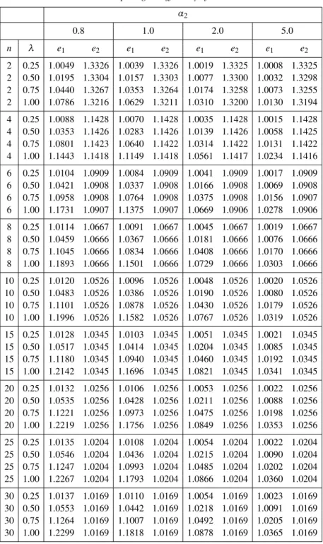
are based numerical computation, and we did not consider LRSS and MERSS schemes. Here, we considern=2(2)10(5)25,α2=0.8,1.0,2.0,5, andλ=±.25,±.5,±.75,±1. In Table 1, we calculate the relative efficiencye1of ˆµRSSto ˜µ, and we can conclude that i) ˜µ is more efficient than ˆµRSS, ii) the efficiency increases with respect to|λ|for fixednandα, iii) the efficiency increases with respect tonfor fixedλandα, and iv) the
efficiency decreases with respect toαfor fixedλandn.
In Table 1, we calculate the relative efficiency e2 of ˆµERSS2 to ˆµRSS, and we can conclude that i) ˆµERSS2 is more efficient than ˆµRSS, ii) the efficiency decreases with respect to|λ|andαfor fixedn, iii) the efficiency decreases with respect tonfor fixed
λandα, iv) the efficiency closes to one for very largen, and v) the efficiency decreases with respect toαfor fixedλandn. Also, ˆµERSS2is more efficient than ˜µ.
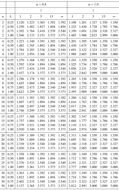
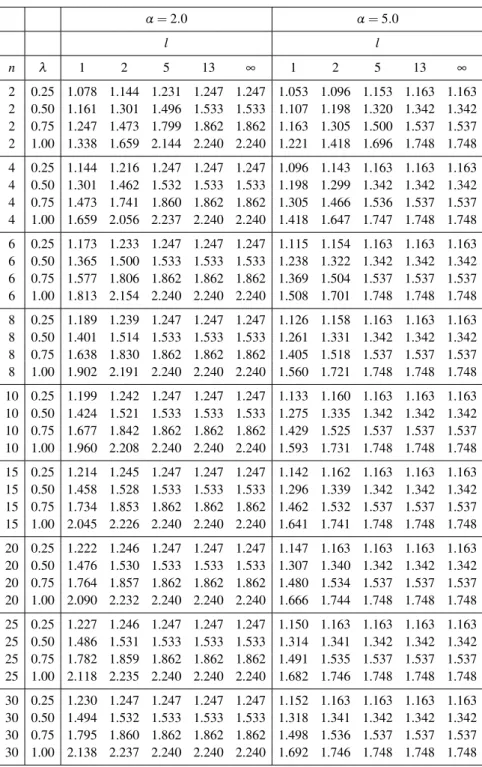
In Tables 2 and 3, for different values forl, we calculate the relative efficiency of
ˆ µMSRSSto ˆµRSS, e5=e(µˆMRRSS|µˆRSS) = C(α2)ξ2nl γnl .
Table 1: Comparing the efficiency of estimations. α2 0.8 1.0 2.0 5.0 n λ e1 e2 e1 e2 e1 e2 e1 e2 2 0.25 1.0049 1.3326 1.0039 1.3326 1.0019 1.3325 1.0008 1.3325 2 0.50 1.0195 1.3304 1.0157 1.3303 1.0077 1.3300 1.0032 1.3298 2 0.75 1.0440 1.3267 1.0353 1.3264 1.0174 1.3258 1.0073 1.3255 2 1.00 1.0786 1.3216 1.0629 1.3211 1.0310 1.3200 1.0130 1.3194 4 0.25 1.0088 1.1428 1.0070 1.1428 1.0035 1.1428 1.0015 1.1428 4 0.50 1.0353 1.1426 1.0283 1.1426 1.0139 1.1426 1.0058 1.1425 4 0.75 1.0801 1.1423 1.0640 1.1422 1.0314 1.1422 1.0131 1.1422 4 1.00 1.1443 1.1418 1.1149 1.1418 1.0561 1.1417 1.0234 1.1416 6 0.25 1.0104 1.0909 1.0084 1.0909 1.0041 1.0909 1.0017 1.0909 6 0.50 1.0421 1.0908 1.0337 1.0908 1.0166 1.0908 1.0069 1.0908 6 0.75 1.0958 1.0908 1.0764 1.0908 1.0375 1.0908 1.0156 1.0907 6 1.00 1.1731 1.0907 1.1375 1.0907 1.0669 1.0906 1.0278 1.0906 8 0.25 1.0114 1.0667 1.0091 1.0667 1.0045 1.0667 1.0019 1.0667 8 0.50 1.0459 1.0666 1.0367 1.0666 1.0181 1.0666 1.0076 1.0666 8 0.75 1.1045 1.0666 1.0834 1.0666 1.0408 1.0666 1.0170 1.0666 8 1.00 1.1893 1.0666 1.1501 1.0666 1.0729 1.0666 1.0303 1.0666 10 0.25 1.0120 1.0526 1.0096 1.0526 1.0048 1.0526 1.0020 1.0526 10 0.50 1.0483 1.0526 1.0386 1.0526 1.0190 1.0526 1.0080 1.0526 10 0.75 1.1101 1.0526 1.0878 1.0526 1.0430 1.0526 1.0179 1.0526 10 1.00 1.1996 1.0526 1.1582 1.0526 1.0767 1.0526 1.0319 1.0526 15 0.25 1.0128 1.0345 1.0103 1.0345 1.0051 1.0345 1.0021 1.0345 15 0.50 1.0517 1.0345 1.0414 1.0345 1.0204 1.0345 1.0085 1.0345 15 0.75 1.1180 1.0345 1.0940 1.0345 1.0460 1.0345 1.0192 1.0345 15 1.00 1.2142 1.0345 1.1696 1.0345 1.0821 1.0345 1.0341 1.0345 20 0.25 1.0132 1.0256 1.0106 1.0256 1.0053 1.0256 1.0022 1.0256 20 0.50 1.0535 1.0256 1.0428 1.0256 1.0211 1.0256 1.0088 1.0256 20 0.75 1.1221 1.0256 1.0973 1.0256 1.0475 1.0256 1.0198 1.0256 20 1.00 1.2219 1.0256 1.1756 1.0256 1.0849 1.0256 1.0353 1.0256 25 0.25 1.0135 1.0204 1.0108 1.0204 1.0054 1.0204 1.0022 1.0204 25 0.50 1.0546 1.0204 1.0436 1.0204 1.0215 1.0204 1.0090 1.0204 25 0.75 1.1247 1.0204 1.0993 1.0204 1.0485 1.0204 1.0202 1.0204 25 1.00 1.2267 1.0204 1.1793 1.0204 1.0866 1.0204 1.0360 1.0204 30 0.25 1.0137 1.0169 1.0110 1.0169 1.0054 1.0169 1.0023 1.0169 30 0.50 1.0553 1.0169 1.0442 1.0169 1.0218 1.0169 1.0091 1.0169 30 0.75 1.1264 1.0169 1.1007 1.0169 1.0492 1.0169 1.0205 1.0169 30 1.00 1.2299 1.0169 1.1818 1.0169 1.0878 1.0169 1.0365 1.0169
Table 2: Comparing the efficiency of estimations. α=0.8 α=1.0 l l n λ 1 2 5 13 ∞ 1 2 5 13 ∞ 2 0.25 1.120 1.223 1.365 1.392 1.392 1.108 1.201 1.327 1.350 1.350 2 0.50 1.250 1.482 1.827 1.894 1.894 1.225 1.430 1.728 1.785 1.786 2 0.75 1.392 1.784 2.410 2.539 2.540 1.350 1.691 2.220 2.326 2.327 2 1.00 1.546 2.133 3.151 3.372 3.373 1.485 1.988 2.823 2.999 3.000 4 0.25 1.223 1.340 1.391 1.392 1.392 1.201 1.305 1.349 1.350 1.350 4 0.50 1.482 1.765 1.892 1.894 1.894 1.430 1.675 1.784 1.786 1.786 4 0.75 1.784 2.293 2.536 2.540 2.540 1.691 2.122 2.323 2.327 2.327 4 1.00 2.133 2.954 3.366 3.373 3.373 1.988 2.665 2.994 3.000 3.000 6 0.25 1.270 1.368 1.392 1.392 1.392 1.242 1.329 1.350 1.350 1.350 6 0.50 1.592 1.834 1.894 1.894 1.894 1.525 1.734 1.785 1.786 1.786 6 0.75 1.977 2.424 2.539 2.540 2.540 1.856 2.231 2.326 2.327 2.327 6 1.00 2.437 3.174 3.372 3.373 3.373 2.242 2.842 2.999 3.000 3.000 8 0.25 1.296 1.378 1.392 1.392 1.392 1.265 1.338 1.350 1.350 1.350 8 0.50 1.655 1.860 1.894 1.894 1.894 1.580 1.756 1.786 1.786 1.786 8 0.75 2.092 2.473 2.540 2.540 2.540 1.953 2.272 2.327 2.327 2.327 8 1.00 2.622 3.259 3.373 3.373 3.373 2.395 2.909 3.000 3.000 3.000 10 0.25 1.313 1.383 1.392 1.392 1.392 1.280 1.342 1.350 1.350 1.350 10 0.50 1.697 1.872 1.894 1.894 1.894 1.616 1.767 1.786 1.786 1.786 10 0.75 2.168 2.497 2.540 2.540 2.540 2.017 2.291 2.327 2.327 2.327 10 1.00 2.746 3.299 3.373 3.373 3.373 2.496 2.941 3.000 3.000 3.000 15 0.25 1.337 1.388 1.392 1.392 1.392 1.302 1.347 1.350 1.350 1.350 15 0.50 1.757 1.884 1.894 1.894 1.894 1.668 1.777 1.786 1.786 1.786 15 0.75 2.279 2.521 2.540 2.540 2.540 2.110 2.311 2.327 2.327 2.327 15 1.00 2.930 3.340 3.373 3.373 3.373 2.645 2.974 3.000 3.000 3.000 20 0.25 1.350 1.389 1.392 1.392 1.392 1.313 1.348 1.350 1.350 1.350 20 0.50 1.789 1.889 1.894 1.894 1.894 1.695 1.781 1.786 1.786 1.786 20 0.75 2.339 2.529 2.540 2.540 2.540 2.160 2.318 2.327 2.327 2.327 20 1.00 3.030 3.354 3.373 3.373 3.373 2.726 2.985 3.000 3.000 3.000 25 0.25 1.358 1.390 1.392 1.392 1.392 1.320 1.349 1.350 1.350 1.350 25 0.50 1.809 1.891 1.894 1.894 1.894 1.712 1.783 1.786 1.786 1.786 25 0.75 2.376 2.533 2.540 2.540 2.540 2.191 2.321 2.327 2.327 2.327 25 1.00 3.093 3.361 3.373 3.373 3.373 2.777 2.990 3.000 3.000 3.000 30 0.25 1.363 1.391 1.392 1.392 1.392 1.325 1.349 1.350 1.350 1.350 30 0.50 1.822 1.892 1.894 1.894 1.894 1.724 1.784 1.786 1.786 1.786 30 0.75 2.402 2.535 2.540 2.540 2.540 2.213 2.323 2.327 2.327 2.327 30 1.00 3.137 3.365 3.373 3.373 3.373 2.812 2.993 3.000 3.000 3.000
Table 3: Comparing the efficiency of estimations. α=2.0 α=5.0 l l n λ 1 2 5 13 ∞ 1 2 5 13 ∞ 2 0.25 1.078 1.144 1.231 1.247 1.247 1.053 1.096 1.153 1.163 1.163 2 0.50 1.161 1.301 1.496 1.533 1.533 1.107 1.198 1.320 1.342 1.342 2 0.75 1.247 1.473 1.799 1.862 1.862 1.163 1.305 1.500 1.537 1.537 2 1.00 1.338 1.659 2.144 2.240 2.240 1.221 1.418 1.696 1.748 1.748 4 0.25 1.144 1.216 1.247 1.247 1.247 1.096 1.143 1.163 1.163 1.163 4 0.50 1.301 1.462 1.532 1.533 1.533 1.198 1.299 1.342 1.342 1.342 4 0.75 1.473 1.741 1.860 1.862 1.862 1.305 1.466 1.536 1.537 1.537 4 1.00 1.659 2.056 2.237 2.240 2.240 1.418 1.647 1.747 1.748 1.748 6 0.25 1.173 1.233 1.247 1.247 1.247 1.115 1.154 1.163 1.163 1.163 6 0.50 1.365 1.500 1.533 1.533 1.533 1.238 1.322 1.342 1.342 1.342 6 0.75 1.577 1.806 1.862 1.862 1.862 1.369 1.504 1.537 1.537 1.537 6 1.00 1.813 2.154 2.240 2.240 2.240 1.508 1.701 1.748 1.748 1.748 8 0.25 1.189 1.239 1.247 1.247 1.247 1.126 1.158 1.163 1.163 1.163 8 0.50 1.401 1.514 1.533 1.533 1.533 1.261 1.331 1.342 1.342 1.342 8 0.75 1.638 1.830 1.862 1.862 1.862 1.405 1.518 1.537 1.537 1.537 8 1.00 1.902 2.191 2.240 2.240 2.240 1.560 1.721 1.748 1.748 1.748 10 0.25 1.199 1.242 1.247 1.247 1.247 1.133 1.160 1.163 1.163 1.163 10 0.50 1.424 1.521 1.533 1.533 1.533 1.275 1.335 1.342 1.342 1.342 10 0.75 1.677 1.842 1.862 1.862 1.862 1.429 1.525 1.537 1.537 1.537 10 1.00 1.960 2.208 2.240 2.240 2.240 1.593 1.731 1.748 1.748 1.748 15 0.25 1.214 1.245 1.247 1.247 1.247 1.142 1.162 1.163 1.163 1.163 15 0.50 1.458 1.528 1.533 1.533 1.533 1.296 1.339 1.342 1.342 1.342 15 0.75 1.734 1.853 1.862 1.862 1.862 1.462 1.532 1.537 1.537 1.537 15 1.00 2.045 2.226 2.240 2.240 2.240 1.641 1.741 1.748 1.748 1.748 20 0.25 1.222 1.246 1.247 1.247 1.247 1.147 1.163 1.163 1.163 1.163 20 0.50 1.476 1.530 1.533 1.533 1.533 1.307 1.340 1.342 1.342 1.342 20 0.75 1.764 1.857 1.862 1.862 1.862 1.480 1.534 1.537 1.537 1.537 20 1.00 2.090 2.232 2.240 2.240 2.240 1.666 1.744 1.748 1.748 1.748 25 0.25 1.227 1.246 1.247 1.247 1.247 1.150 1.163 1.163 1.163 1.163 25 0.50 1.486 1.531 1.533 1.533 1.533 1.314 1.341 1.342 1.342 1.342 25 0.75 1.782 1.859 1.862 1.862 1.862 1.491 1.535 1.537 1.537 1.537 25 1.00 2.118 2.235 2.240 2.240 2.240 1.682 1.746 1.748 1.748 1.748 30 0.25 1.230 1.247 1.247 1.247 1.247 1.152 1.163 1.163 1.163 1.163 30 0.50 1.494 1.532 1.533 1.533 1.533 1.318 1.341 1.342 1.342 1.342 30 0.75 1.795 1.860 1.862 1.862 1.862 1.498 1.536 1.537 1.537 1.537 30 1.00 2.138 2.237 2.240 2.240 2.240 1.692 1.746 1.748 1.748 1.748
Note that e5 is the relative efficiency of ˆµUSSRSS to ˆµRSS, i.e. e4, whenl=∞. We can conclude that i) ˆµMSRSSis more efficient than ˆµRSS, ii) the efficiency increases with
respect to λ>0 for fixed n andα, iii) the efficiency increases with respect to n for
fixedλandα, and iv) the efficiency decreases with respect toαfor fixedλandn. Also,
the efficiency increases when the number of stages,l, increases, and ˆµUSSRSS is more
efficient than ˆµMSRSSfor alll.
Acknowledgements
The authors would like to thank an anonymous reviewer of this journal for many constructive suggestions and comments for improving this manuscript.
References
Al-Nasser, A. D. (2007). L ranked set sampling: A generalization procedure for robust visual sampling. Communications in Statistics-Simulation and Computation, 36, 33–43.
Al-Nasser, A. D. and Mustafa, A. B. (2009). Robust extreme ranked set sampling. Journal of Statistical Computation and Simulation, 79, 859–867.
Al-Odat, M. and Al-Saleh, M. F. (2001). A variation of ranked set sampling.Journal of Applied Statistical Science, 10, 137–146.
Al-Saleh, M. F. (2004). Steady-state ranked set sampling and parametric estimation.Journal of Statistical Planning and Inference, 123, 83–95.
Al-Saleh, M. F. and Al-Ananbeh, A. M. (2007). Estimation of the means of the bivariate normal using moving extreme ranked set sampling with concomitant variable.Statistical Papers, 48, 179–195. Al-Saleh, M. F. and Al-Kadiri, M. A. (2000). Double-ranked set sampling.Statistics and Probability
Let-ters, 48, 205–212.
Al-Saleh, M. F. and Al-Omari, A. I. (2002). Multistage ranked set sampling.Journal of Statistical Planning and Inference, 102, 273–286.
Al-Saleh, M. F. and Diab, Y. A. (2009). Estimation of the parameters of Downton’s bivariate exponential distribution using ranked set sampling scheme.Journal of Statistical Planning and Inference, 139, 277–286.
Barnett, V. and Moore, K. (1997). Best linear unbiased estimates in ranked-set sampling with particular reference to imperfect ordering.Journal of Applied Statistics, 24, 697–710.
Chacko, M. and Thomas, P. Y. (2008). Estimation of a parameter of Morgenstern type bivariate exponential distribution by ranked set sampling.Annals of the Institute of Statistical Mathematics, 60, 301–318. Chen, Z., Bai, Z. and Sinha, B. (2004).Lecture Notes in Statistics, Ranked Set Sampling: Theory and
Ap-plications. Springer, New York.
David, H. A. and Nagaraja, H. (2003).Order Statistics. John Wiley and Sons.
Jemain, A. A. and Al-Omari, A. I. (2006). Double quartile ranked set samples.Pakistan Journal of Statis-tics, 22, 217–228.
McIntyre, G. A. (1952). A method for unbiased selective sampling, using ranked sets.Australian Journal of Agricultural Research, 3, 385–390.
Muttlak, H. A. (1997). Median ranked set sampling.Journal of Applied Statistical Sciences, 6, 245–255. Muttlak, H. A. (2003). Modified ranked set sampling methods.Pakistan Journal of Statistics, 19, 315–324.
Samawi, H. M., Ahmed, M. S. and Abu-Dayyeh, W. (1996). Estimating the population mean using extreme ranked set sampling.Biometrical Journal, 38, 577–586.
Scaria, J. and Nair, N. U. (1999). On concomitants of order statistics from Morgenstern family.Biometrical Journal, 41, 483–489.
Sinha, B. K., Sinha, B. K. and Purkayastha, S. (1996). On some aspects of ranked set sampling for estima-tion of normal and exponential parameters.Statistics and Decisions, 14, 223–240.
Stokes, S. L. (1977). Ranked set sampling with concomitant variables.Communications in Statistics-Theory and Methods, 6, 1207–1211.
Stokes, S. L. (1980). Inferences on the correlation coefficient in bivariate normal populations from ranked set samples.Journal of the American Statistical Association, 75, 989–995.
Tahmasebi, S. and Jafari, A. A. (2012). Estimation of a scale parameter of Morgenstern type bivariate uniform distribution by ranked set sampling.Journal of Data Science, 10, 129–141.
Tahmasebi, S. and Jafari, A. A. (2013). Concomitants of order statistics and record values from Morgen-stern type bivariate generalized exponential distribution.Bulletin of the Malaysian Mathematical Sciences Society, (Accepted for publication).
Takahasi, K. and Wakimoto, K. (1968). On unbiased estimates of the population mean based on the sample stratified by means of ordering.Annals of the Institute of Statistical Mathematics, 20, 1–31. Yu, P. L. and Tam, C. Y. (2002). Ranked set sampling in the presence of censored data.Environmetrics, 13,