FPGA-BASED CASCADE SUPPORT VECTOR MACHINE WITH INTEGRATED TRAINING
A Thesis by YEN-JU LIN
Submitted to the Office of Graduate and Professional Studies of Texas A&M University
in partial fulfillment of the requirements for the degree of MASTER OF SCIENCE
Chair of Committee, Peng Li Committee Members, Gwan Choi
Ricardo Gutierrez-Osuna Head of Department, Miroslav M. Begovic
August 2016
Major Subject: Computer Engineering
ii ABSTRACT
Machine learning algorithms allow us to reason about and analyze large amounts of data. The support vector machine (SVM) is one popular learning algorithm, which has been applied to a broad range of applications. To this end, hardware-based SVM processors are very appealing due to their improved runtime and energy efficiency.
This research proposes an FPGA-based parallel support vector machine processor, which is capable of processing multi-dimensional data sets. The proposed FPGA SVM is based upon the cascade SVM algorithm, which is leveraged to allow efficient parallel processing of data on the FPGA platform, leading to significant processing efficiency.
iii DEDICATION
I would like to dedicate my thesis work to my family, for my parents and grandmother’s selfless support and my brother’s academic help since we were kids to now, which has made my graduate studies and accomplishment possible.
iv
ACKNOWLEDGEMENTS
I would like to thank my committee chair, Dr. Li, my committee members, Dr. Choi, Dr. Gutierrez-Osuna, and my committee substitute Dr. Khatri, for their help and guidance through this research work.
I would also like to thank Qian Wang, Youjie Li and other peers from Dr. Li’s research group, thanks to all for their help and time spent in discussions with me. Finally, I would like to thank all of my peers and friends, both present and past, for helping and supporting me throughout my graduate studies.
v
NOMENCLATURE
ANN Artificial Neural Network
ASIC Application-Specific Integrated Circuit
AXI Advanced eXtensible Interface
BRAM Block RAM
CF card Compact Flash Card
FAT File Allocation Table
FPGA Field-Programmable Gate Array
GPU Graphics Processing Units
KKT Karush-Kuhn-Tucker
PCIe Peripheral Component Interconnect Express
SMO Sequential Minimal Optimization
SV Support Vector
SVM Support Vector Machine
System ACE System Advanced Configuration Environment UART Universal Asynchronous Receiver/Transmitter
vi TABLE OF CONTENTS Page ABSTRACT ... ii DEDICATION ... iii ACKNOWLEDGEMENTS ... iv NOMENCLATURE ... v TABLE OF CONTENTS ... vi
LIST OF FIGURES ... viii
LIST OF TABLES ... x
1. INTRODUCTION ... 1
1.1 Background and Motivation ... 1
1.2 Classification in Machine Learning ... 3
1.3 Overview of Support Vector Machine ... 6
1.3.1 Applications ... 7
1.3.2 Hardware Implementation ... 10
1.4 Research Objective ... 11
2. ALGORITHMS OF SUPPORT VECTOR MACHINE ... 13
2.1 Basic Support Vector Machine ... 13
2.1.1 Kernel Method ... 17
2.1.2 Classification Checking ... 18
2.2 Cascade Support Vector Machine ... 20
3. HARDWARE IMPLEMENTATIONS ... 23
3.1 Support Vector Machine Structure ... 23
3.1.1 SVM Unit Structure ... 23
3.1.2 Cascade SVM Unit Setup ... 26
3.2 UART System Implementation ... 29
3.2.1 Hardware Structure Overview ... 30
vii
3.3 Memory Card System Implementation ... 37
3.3.1 Hardware Structure Overview ... 38
3.3.2 Experimental Setup of the FPGA ... 43
3.4 Memory Improvement and Comparison ... 45
4. EXPERIMENTAL RESULTS ... 47
4.1 Runtime Comparison ... 47
4.1.1 Hardware Speedup ... 49
4.1.2 Basic and Cascade SVM Comparison ... 50
4.2 Non-artificial Data Sets Training and Execution Time Comparison ... 51
4.2.1 Pima Indians Diabetes Data Set ... 52
4.2.2 Vertebral Column Data Set ... 53
4.2.3 Mammographic Data Set ... 54
4.2.4 Execution Time Discussion ... 55
4.3 Device Utilization and Power/Energy Consumption ... 60
5. SUMMARY AND CONCLUSIONS ... 63
5.1 Summary and Conclusions ... 63
5.2 Future Work ... 64
viii
LIST OF FIGURES
Page
Figure 1.1 A demonstration of linear classification ... 5
Figure 1.2 A training model with binary classification data set ... 7
Figure 1.3 A difficult separating training model ... 8
Figure 2.1 Hyperplane demonstration ... 13
Figure 2.2 Soft-margin SVM with SVs in darker shades ... 16
Figure 2.3 Cascade SVM versus single SVM ... 21
Figure 3.1 A SVM unit structure ... 23
Figure 3.2 Data storage demonstration ... 24
Figure 3.3 A two dimension training model and its result ... 25
Figure 3.4 A cascade SVM structure ... 27
Figure 3.5 A reusable cascade SVM unit structure ... 28
Figure 3.6 Memory management units implementation ... 28
Figure 3.7 UART data frame... 30
Figure 3.8 Hardware structure in the FPGA with UART ... 31
Figure 3.9 An 8-dimension SVM unit. ... 34
Figure 3.10 Slices registers of distribution for two dimensions SVM unit ... 35
Figure 3.11 Slices registers distribution a two dimensions basic SVM FPGA implementation ... 36
Figure 3.12 Device utilization in different dimensions ... 37
ix
Figure 3.14 A BRAM buffer ... 39
Figure 3.15 Data storage change ... 40
Figure 3.16 Data division in the Microblaze control ... 41
Figure 3.17 Data path ... 43
Figure 3.18 Possible data size in the built-in BRAMs ... 45
Figure 4.1 A training result for a training model using a data set with 100 samples in -UART version of cascade SVM training ... 48
Figure 4.2 Runtime of 50, 100, 200 samples ... 49
Figure 4.3 Execution time distributions in UART implementation for benchmark 1 ... 56
Figure 4.4 Execution time distributions in memory card implementation for -benchmark 1 ... 57
x
LIST OF TABLES
Page
Table 4.1 Comparison of classification time ... 50
Table 4.2 Training runtime comparison ... 51
Table 4.3 The memory card implementation execution time ... 59
Table 4.4 Device utilization ... 60
Table 4.5 Device utilization without the Microblaze system ... 61
1
1. INTRODUCTION 1.1 Background and Motivation
In the world nowadays, human comes across with a lot of information every day. A biological research may have more than millions of data at a time. For example, in order to understand how computed tomography scans influence health, it requires the health records tracking for 11 millions of people [1]. With such amount of data, it shows its consequence and influence on human bodies. As another example, in meteorology studies, a lot of climate data are collected to understand the weather in recent years [2]. By long term climate changes and the current environment observation, future climate changes and possible dangers are predicted. These data show important information about the unknown in the world, while machine learning algorithms show a way to explore and make use of those data.
By machine learning algorithms, the relationship between those data and their outcomes are disclosed. Therefore, results of new samples can be predicted, while features and behaviors of original data can be understood. For example, by collecting common features of cancer patients can predict the tendency in cancer. With machine learning algorithms, those parts of gene, which play an important role on cancer development, can be distinguished from a huge amount of other irrelevant gene parts [3]. For another example, it is also applied in the radar image reading, while these radar images show where the oil spitted causing the environmental issues are [4]. Those radar images were observed and studied manually in the past, it took experience and heavy
2
work load to identify current situation in radar images. However, with machine learning technology, the oil spitted can be detected from radar images in an efficient way and at an early stage. Therefore people are able to take actions immediately to the situation and stop worsening the damage to the ocean.
Machine learning technology has these benefits in the research purpose; however, it requires a huge amount of time, from hours to weeks, and a lot of power to make use of these data in software implementations. To solve these issues and make machine learning algorithms more accessible, researchers have been dedicated to shorting the runtime and reducing power consumptions. For instance, it takes around 5 hours to train a model over a data set with 481,000 samples in a traditional machine learning algorithm. By improving the algorithm, the runtime may be reduced from 5 hours to less than 1 minute [5]. Apart from runtime speedup, some research has been done on power reduction by using different technology and designing power-aware algorithms [6].
On the other hand, a specific designed hardware is faster and consumes less power compared with same software logic performed on a general purpose CPU. Here are the reasons. Firstly, for the same logic, a hardware implementation is able to implement it in a parallel manner, where a parallel architecture is explored. Secondly, a hardware implementation does not need instruction memories to store computation instructions, which is necessary for the software. In the hardware, only those logic gates required by the design exist, but for software, it requires all the general logics implementation in a general purpose CPU.
3
To enjoy those benefits from machine learning algorithms and hardware implementations, a specific ASIC design of support vector machine algorithm (SVM) is developed in the previous research [7]. It is able to achieve five hundred times speedup and approximately twenty thousand times energy reduction compared with a software SVM algorithm. But due to the limited storage and the restricted design flow of the ASIC platform, only limited amount of data and those training models with two dimensions can easily be trained. If the structure needs to be modified for higher dimensions or improved, it requires a lot of time for modification and testing. Therefore, the main motivations and challenges for this thesis research are to maintain the benefits from the hardware design and a flexible version of hardware implementation.
1.2 Classification in Machine Learning
With machine learning algorithms, different kinds of training models can be trained and used, in order to get the specific feature in a model.
There are few kinds of machine learning algorithms in terms of the outputs relation with inputs in the training model, which are classification, regression, clustering, density estimation and dimension reduction [8]. With different kinds of training models, the corresponding learning algorithm is chosen. For example, a regression method predicts the output from a new sample in a continuous training model [9]. On the other hand, by clustering, it distinguishes different kinds unknown of data types for a given training model. The clustering method and regression can be applied in decease detection technology [10].
4
Apart from other methods, for the data set of a training model with known classifications, a new sample can be assigned to one of those classifications with classification algorithms. With the help of classification algorithms, classifications of unknown samples are predicted from the training model. There are different kinds of classification algorithms, and the linear classification is one of the commonly used classification algorithms. A linear classifier separates data according to the linear combination of samples from the training model.
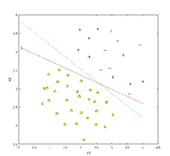
From Figure 1.1, two linear classifications have been performed to separate different classifications of a training model. Because of the complexity of computation in linear combinations, it requires less time in the training process to reach the similar accuracy compared with a non-linear classifier. Though it is able to approximate a non-linear training model as a linear classification problem, it is not applicable for those training models which have complicated non-linear characteristic [11].
5
Figure 1.1 A demonstration of linear classification
For example, with linear classifiers, text categorization can be performed in a training model, which is able to separate text contents [12]. This is widely used in separating spam emails and regular emails for users in a huge amount of incoming emails.
On the other hand, artificial neural network (ANN) is also a widely used classification learning algorithm. It is inspired by the neural network of animals, in animals’ brain, a series of connected neurons exchange messages by transmitting electrics signals. With those signals, animals are able to react to messages from outside world, including thinking, acting with emotions, and learning. By the concept of neurons, ANN constructs a large numbers of nodes, named neurons, connecting with one another. In each connection, it has a numerical number working as a weighed number. With those
6
nodes and weighed connections, it is able to adjust to the incoming unknown data, aiming to working as a biological neuron network [13]. For example, lung cancers are able to be identified via ANN [14]. By obtaining the image of lungs, it is possible to tell whether it is a healthy cell or a cancer cell by ANN.
With these classification algorithms in machine learning technology, it is possible to learn from those data, and explore the unknown of the world. Linear classifiers present a relative fast and easy way to distinguish a training model compared with non-linear classifiers. By the inspiration of biological neuron networks, ANN learns from training models. These algorithms contribute to all the aspects in the world, from separating spam emails in email boxes, to identifying cancer cells.
Finally, another widely used algorithm in classification is the support vector machine, which is the algorithm used in the research. More details would be addressed in the next section.
1.3 Overview of Support Vector Machine
Support vector machine, known as SVM, is one of the commonly used learning algorithms in classification and it predicts future samples from the training model [15]. SVM analyzes data for classification analysis; it distinguishes different features in a training model and predicts the result. That is, for instance, for the data set of a training model, it is able to assign a new sample into one of those different categories after the SVM training process. In this research, it is a parallel SVM algorithm implemented by the FPGA.
7
1.3.1 Applications
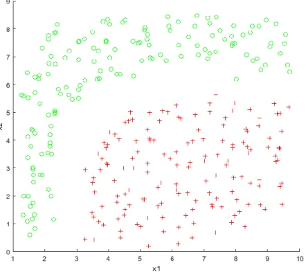
There are some typical uses for SVMs. For example, it separates a training model with a binary data set according to its classifications. If there is a new sample, it is able to predict the classification of that new sample. In Figure 1.2, it is a training model with two kinds of classifications, circle and plus sign. With SVM, whether circle or plus sign classification of a new sample can be predicted.
Figure 1.2 A training model with binary classification data set
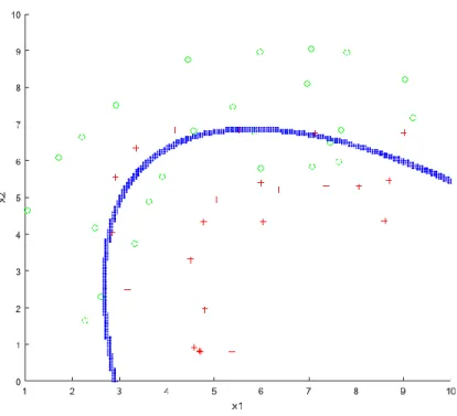
On the other hand, for a training model which is not easily separable, SVM is still able to generate a suitable boundary for the training model according to the user’s
8
need. By modifying the setup in the algorithm, the boundary is tuned in order to have a separating boundary that meets the requirement.
Figure 1.3 A difficult separating training model
In the Figure 1.3, these two categories are not as clearly divided in the Figure 1.2. However, it is still able to generate a boundary that separates most of the samples by SVM.
With the help of SVM, it is not only possible to separate linear training models as linear classifiers, but it is also possible to separate those training models in a more complex form, like Figure 1.3.
9
For example, by SVM, tissues are separated accurately according to the difference in normal and cancer tissues. Furthermore, with the help of SVM, it is also able to distinguish mistakenly labels tissues. Finally, it separates not only normal tissues and cancer ovarian tissues, but also those tissues from other part of the human body [15]. With more accurate ways proposed to distinguish cancers and diseases, it provides more precise and correct treatments compared with the past. Therefore more lives can be saved in the future as the technology developed.
Apart from medical use as the example above, SVM is also used in image retrieval [16]. With a big database of images, it is time-consuming to label and make description for each image manually. And it is also difficult for image searchers to be specific on picture features, while colors or sizes of the picture may not play an important role in terms of searching. For example, if an image of a rabbit is needed, the image of a rabbit may have different colors in the background or the rabbit itself has more than one color according to its species; on the other hand, the image may be a hand drawing rabbit uploaded by a scanner with low quality, it may also be a high quality picture taken by a professional camera. With SVM, it is able to create a boundary between targeted images and other images in the database. Therefore, it saves time and the work of labeling images manually, and it has a better outcome if images are found with a different classification way from labels. This method helps in the picture preservation and search.
From these applications of SVM, SVM plays an important role in current technology and human lives. Therefore to make SVM more efficient in data training,
10
researchers have dedicated their time and efforts to transfer it from the software platform to hardware implementations in order to enjoy benefits of the hardware characteristics.
1.3.2 Hardware Implementation
Because of time reduction from hardware implementations and benefits of SVM achieved in research works, some research has been proposed on hardware implementations of SVM.
For example, an analog VLSI design of a SVM algorithm has been proposed [17]. By implementing the kernel of a SVM algorithm, it provides a faster solution for the SVM algorithm. On the other hand, with the trade-off with power, it is also a power efficient solution. With a SVM algorithm implemented on chip, it is portable and flexible for users. In order to have a great power efficiency improvement, another design in the analog VLSI of SVM has been proposed [18]. Instead of a traditional MOS transistor dependence method, by adopting the margin propagation in design gives the analog VLSI implementation a better performance in power efficiency.
Apart from analog VLSI, some works in digital architecture are proposed, by implementing a SVM algorithm in other ways, different benefits are achieved. By implementing the sequential minimal optimization SVM in a digital VLSI, it provides the retraining flexibility to the implementation, noted that it is only applicable for a linear kernel [19]. In the future, it may be further developed as a system on a chip. With a system on a chip implemented SVM, it gives more opportunities and convenience for those using SVM algorithms.
11
Finally, the FPGA is another popular platform to implement SVM in hardware. By implementing SVM in the FPGA, it achieves a better precision and resolution compared with SVM in analog VLSI implementations [20]. Moreover, some SVM implementations on the FPGA focus on the acceleration of the classification process [21]. On the other hand, the graphics processing unit, GPU, is also another popular implementation choice, which has also been used in the SVM implementation [22]. By comparing the FPGA and the GPU in SVM implementation, different implementations have a better performance in different kinds of training models [23]. The FPGA implementation gave a better performance in chunking technology of SVM, while GPU is less limited by the dimension increment.
There have been a lot of researchers dedicated to hardware implementations on SVM with different methods, the speedup have been achieved from previous works. A lot of works have been focus on the internal training process acceleration; on the other hand, by speeding up the algorithm itself is also an approach to improve the training efficiency. This research is based on a previous work that focused on algorithm speedup [7].
1.4 Research Objective
From previous discussions, SVM is known as an effective way for data classifications. With the hardware implementation, it is also able to have a better performance in power and runtime.
12
In the previous studies of SVM hardware implementations, it has the benefits of time reduction and power efficiency by implementing the cascade SVM algorithm in hardware; however, there are certain limitations of it. It only trains certain dimensions of a training model, and it has limited data storage, which led to a difficulty of real world data training.
The goal of this research is as followed, first, expanding the possible data dimensions for training in a faster manner, in order to train with real world data. Second, increase the internal data storage to work with large training models. By migration of the design from the ASIC platform to the FPGA, the above goals are able to be achieved.
13
2. ALGORITHMS OF SUPPORT VECTOR MACHINE 2.1 Basic Support Vector Machine
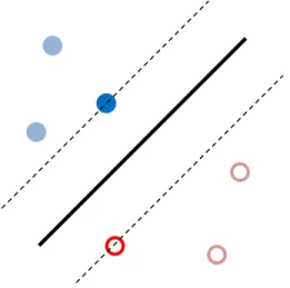
The hardware implementation is based on the SVM learning algorithm as discussed in the previous section. In order to separate samples and predict the classifications of unknown samples, the goal of SVM is to find a separating hyperplane between those close samples with the largest distance to the hyperplane [24].
Figure 2.1 Hyperplane demonstration
In Figure 2.1, it is a demonstration of a hyperplane between two different classifications of samples. To have a precise separation from samples of different categories, the close samples to each other in different categories are chosen as the
14
starting points and form a boundary of their categories. The hyperplane is between those boundaries, in the Figure 2.1, the hyperplane lies between the boundaries of these two different categories, namely circle and ring. Therefore, only some of samples contribute to the hyperplane formulation, which are called support vectors, SVs.
Firstly, a sample and its classification are shown in below:
(𝑥⃑⃑⃑ , 𝑦𝑖 𝑖), 𝑦𝑖 = {+1, −1}, 𝑖 = 1,2, … 𝑁
where 𝑥⃑⃑⃑ 𝑖 is the input vector, and 𝑦𝑖 is the corresponding classification.
By assuming a mapping function 𝜙(𝑥) between samples and classifications, the relationship between an input sample and its classification can be written as these two equations:
{ 𝑦 = +1, 𝑤 ∙ 𝜙(𝑥) + 𝑏 ≥ 1 𝑦 = −1, 𝑤 ∙ 𝜙(𝑥) + 𝑏 ≤ −1
where w is the normal toward the separating plane.
To find the hyperplane, the relation between 𝑥⃑⃑⃑ 𝑖 and 𝑦𝑖 is obtained as following:
𝑓 = 𝑦𝑖(𝑤 ∙ 𝜙(𝑥𝑖) + 𝑏)
where b is the bias. And the distance from close samples to the hyperplane, named margin, is 2/‖𝑤‖.
15 As a result, the optimization problem is:
𝑚𝑖𝑛𝑤,𝑏‖𝑤‖
2
2
which is subject to 𝑦𝑖(𝑤 ∙ 𝜙(𝑥𝑖) + 𝑏) = 1.
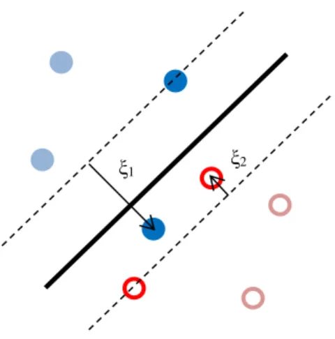
However, not all training models have a strictly separated hyperplane. Therefore a soft-margin SVM is proposed in terms of the trade-off between the margin and errors. For the tolerance of training errors in this research, a soft-margin SVM is used with the optimization problem as below:
𝑚𝑖𝑛𝑤,𝜉,𝑏‖𝑤‖
2
2 + 𝐶 ∑ 𝜉𝑖
𝑁
𝑖=1
The additional 𝜉𝑖 in the new optimization problem is the slack variable, which gives the flexibility for samples to violate the hyperplane. C is a constant controlling the trade-off between margin accuracy and error tolerance. Figure 2.2 demonstrates the error tolerance of two different categories and its hyperplane. The SVs are all the samples inside the dash lines, which makes the new optimization problem is now subject to
16
Figure 2.2 Soft-margin SVM with SVs in darker shades
After the optimization problem is obtained, its Lagrangian problem is shown as below: 𝑀𝑖𝑛 𝐿𝑝(𝑤, 𝑏, 𝛼𝑖) =‖𝑤‖2 2 − ∑ 𝛼𝑖(𝑦𝑖 𝑁 𝑖=1 (𝑤 ∙ 𝜙(𝑥𝑖) + 𝑏)-1)) 𝑠. 𝑡. 𝛼𝑖 ≥ 0
and the dual problem:
Max ∑ 𝛼𝑖 −1 2 𝑁 𝑖=1 ∑ ∑ 𝛼𝑖 𝑁 𝑗=1 𝛼𝑗𝑦𝑖𝑦𝑗𝑘(𝑥𝑖, 𝑥𝑗) 𝑁 𝑖=1 𝑠. 𝑡. 𝐶 ≥ 𝛼𝑖 ≥ 0 and ∑𝑁𝑗=1𝛼𝑖𝑦𝑖 = 0
From the dual problem, a kernel function 𝑘(𝑥𝑖, 𝑥𝑗) is introduced from the mapping function. In order to find the separating plane and solve the problem, the kernel method is introduced here.
17
2.1.1 Kernel Method
The kernel method provides a measurement between two similar vectors and ensures the optimization problem is convex and unique. It gives a better way to find the relationship in different samples of the training model, and it is mostly used in SVM training [25].
To decide the decision boundary of a classification training model, there are many different kinds of kernel methods. For example, a linear kernel is widely used in SVM. It is able to determine a less complicated model and generate a boundary. For more complex models or higher accuracy requirements, the Gaussian kernel is a popular kernel, which is also used in this research. Apart from these two kernels, there are other kernels also used in SVM, including Fisher kernel and Graph kernel.
A general kernel is defined as k(𝑥𝑖, 𝑥𝑗) = ϕ(𝑥⃑⃑⃑ ) ∙ ϕ(𝑥𝑖 ⃑⃑⃑ )𝑗 , it gives the relation of samples between each other and their mapping function. The Gaussian kernel is used in this research as k(𝑥𝑖, 𝑥𝑗) = exp (−γ‖𝑥⃑⃑⃑ − 𝑥𝑖 ⃑⃑⃑ ‖𝑗 2). In the Gaussian kernel computation, an exponential computation is involved. Unlike linear kernels or polynomial kernels, the Gaussian kernel is not easy and straightforward to be implemented by adders and multipliers.
For hardware implementations, a hardware friendly kernel has been proposed, which remains good performance in many cases [26]. It is an analog circuit implementation proposed in substitute of the Gaussian kernel. However, the Gaussian
18
kernel is still used in this research; the detailed implementation is provided in section 3.1.1.
With the help of the kernel method, it is possible to solve the Lagrangian problem and its dual problem of SVM in section 2.1. By substituting the kernel function
k(𝑥𝑖, 𝑥𝑗) with a Gaussian kernel in the Lagrangian dual problem, the problem is rewritten as below: Max ∑ 𝛼𝑖−12 𝑁 𝑖=1 ∑ ∑ 𝛼𝑖 𝑁 𝑗=1 𝛼𝑗𝑦𝑖𝑦𝑗exp (−γ‖𝑥⃑⃑⃑ − 𝑥𝑖 ⃑⃑⃑ ‖𝑗 2 ) 𝑁 𝑖=1 𝑠. 𝑡. 𝐶 ≥ 𝛼𝑖 ≥ 0 and ∑𝑁𝑗=1𝛼𝑖𝑦𝑖 = 0
By finding 𝛼𝑖, it would lead to SVs, which would be discussed in the next section.
2.1.2 Classification Checking
In SVM learning algorithms, the sequential minimal optimization (SMO) is one of the popular algorithms to solve the optimization problems in SVMs [27]. SMO algorithm is able to solve the above function in an iterative manner. By computing multipliers in pair, it is able to solve the Lagrangian problem efficiently. However, in this research, the gradient ascent method is chosen to solve the above optimization problem, which is more hardware friendly [26]. Firstly, the above problem can be checked by Karush-Kuhn-Tucker (KKT) conditions. With the help of KKT conditions, the α values are able to be determined.
19
The KKT conditions indicate that for a solution in the nonlinear problem to be optimal, its inequality constraints are no longer existed [28]. Consider a nonlinear problem:
Max f(x)
s. t. 𝑔𝑖(x) ≤ 0, ℎ𝑗(𝑥) = 0
If it has an optimal solution, which must satisfy the following conditions:
∇f(𝑥∗) = ∑ 𝜇 𝑖∇𝑔𝑖(𝑥∗) 𝑚 𝑖=1 + ∑𝑙 𝜆𝑗∇ℎ𝑗(𝑥∗) 𝑗=1 m=0
For minimum problems, the left side of the first condition is −∇f(𝑥∗) , instead of
∇f(𝑥∗).
By KKT conditions, the optimal solutions can be found for nonlinear problems. For example, convex optimization methods are very common in communications or signal processing. To find the optimal, KKT conditions are used for these methods [29]. For here, to satisfy KKT conditions, it requires the product of Lagrangian parameters and their constraints to be zero, which is
𝛼𝑖(𝑦𝑖(𝑤𝑇∙ 𝜙(𝑥⃑⃑⃑ ) + 𝑏) − 1 + 𝜉𝑖 𝑖) = 0, 𝛽𝑖𝜉𝑖 = 0.
𝛽𝑖 is the Lagrangian variable for 𝜉𝑖. Therefore KKT conditions of the soft-margin SVM are shown in below:
20 { 𝛼𝑖 = 0 𝑦𝑖(𝑤𝑇∙ 𝜙(𝑥 𝑖 ⃑⃑⃑ ) + 𝑏) ≥ 1 0 < 𝛼𝑖 < 𝐶 𝑦𝑖(𝑤𝑇∙ 𝜙(𝑥 𝑖 ⃑⃑⃑ ) + 𝑏) = 1 𝛼𝑖 = 𝐶 𝑦𝑖(𝑤𝑇∙ 𝜙(𝑥 𝑖 ⃑⃑⃑ ) + 𝑏) ≤ 1
With the relation between the hyperplane and samples, w value is written as
𝑤 = ∑𝑁𝑖=1𝛼𝑖𝑦𝑖𝜙(𝑥⃑⃑⃑ )𝑖 and b is the bias mentioned before. From KKT conditions discussed above, if 𝛼𝑖 = 0, it is not a SV, if 𝛼𝑖 = 𝐶 it is a SV with error tolerance, and finally if 0 < 𝛼𝑖 < 𝐶 , the sample is right on the hyperplane.
From the above process, if 𝛼𝑖 is determined for every sample, the hyperplane can be found and classifications of future samples are able to be predicted. For a new sample 𝑥 , by computing its relation with SVs:
f(𝑥 ) = ∑ 𝛼𝑆𝑉
𝑁𝑆𝑉
𝑖=1
𝑦𝑆𝑉𝐾(𝑥 , 𝑥⃑⃑⃑⃑⃑⃑ )𝑆𝑉
if f(𝑥 ) > 0, its classification is determined as +1, else it is −1.
Therefore, in the hardware implementation, α value is the final result after the training process finishes. The whole process of training is based on iterations of finding SVs and eliminates non-SVs; therefore it may take a long time of training if the training model has a huge amount of data.
2.2 Cascade Support Vector Machine
From the basic SVM discussed in the previous section, it shows that only SVs contribute to the hyperplane, most of the samples in the data set of a training model are non-SVs. Therefore, in the cascade SVM, it eliminates non-SVs at the early stage, which speeds up the whole training process [30].
21
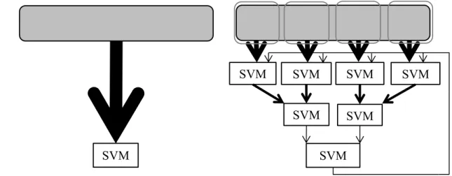
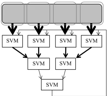
The cascade SVM is implemented in the following manner. First, the data set of a training model is spit into smaller subsets, and those subsets are trained simultaneously. After each subset is trained, SVs from those subsets are fed to SVM units in the next layer for a combined training. This progress is repeated until all subsets are combined and trained. After it reaches the last training process, training results will be fed back for KKT conditions checking. To achieve the design, multiple SVM units are needed, which are placed as a hierarchical structure as Figure 2.3.
Figure 2.3 Cascade SVM versus single SVM
For example, by separating a large data set into four smaller subsets, which is shown in Figure 2.3, those four data sets are trained at the same time. After each training process, the next layer has less samples to train compared with the previous layer, due to
Single SVM SVM SVM SVM SVM SVM SVM SVM SVM Cascade SVM
22
the elimination at the previous layer. Also, since the training process is in quadratic, even though it trains three times for three layers, it is still faster than training all samples at one time.
There are some implementations of the cascade SVM showed a great speedup compared with a basic SVM. For instance, with the implementation of the cascade SVM, the training time for a training model of a data set with 27,000 samples can be reduced from 70 hours to 3 minutes [31]. That is, it has a 1400 times speedup compared with the previous training method.
Though from the aspect of structure, more SVM units are required in order to achieve the parallel computation and multiple layers training compared with a basic SVM, the significance in speedup shows the great benefit of using the cascade SVM instead of a basic SVM.
23
3. HARDWARE IMPLEMENTATIONS 3.1 Support Vector Machine Structure
The main hardware architecture is based on the previous ASIC design [7]. In this section, with the original structure as a starting point, other versions implemented in the FPGA are proposed.
3.1.1 SVM Unit Structure
For a single and basic SVM discussed as before, apart from the internal computation module, it has an address generator for memory access and a lookup table for exponential computations.
Figure 3.1 A SVM unit structure Yi,j Xi1,j1 Xi2,j2 α SVM Multiplier Multiplier Computation Lookup Table Address Generator α
24
The Figure 3.1 shows the overall structure of a SVM unit design. Firstly, a sample is stored in sequence as followed: its classification Y, its first dimension data X1,
its second dimension data X2, and the corresponded α value which is initialized as 0.
According to the address generator, the SVM unit has these four values of a sample. To compute the corresponding α value, other samples are also entered in a same manner. After samples are entered, the computation proceeds to the further computation.
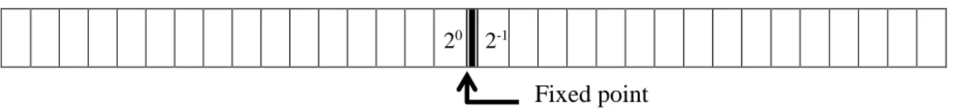
A fixed multiplier is also used in the computation. The fixed multiplier is designed specifically according to the data storage in Figure 3.2. Data is stored as a 32 bits number in two’s complement, which is defined as a fixed point number with 16 bits before the fixed point in Figure 3.2, and 16 bits after the fixed point. That is, the minimal number of a positive number is 2-16. The storage demonstration is shown as Figure 3.2, which shows the precision and implementation of the fixed point data storage design.
Figure 3.2 Data storage demonstration
The kernel method is an important part in SVMs as discussed in the previous section. Although as mentioned in 2.1.1, some specific kernels designed for hardware have been proposed, to ensure the performance in a SVM unit, the Gaussian kernel is used here. To implement the exponential function in Gaussian kernel computation, a lookup table is added. After all the dimensions of the sample and its corresponding
Fixed point
25
compared sample are computed, the value is fed into the lookup table module; the result of Gaussian kernel is further obtained.
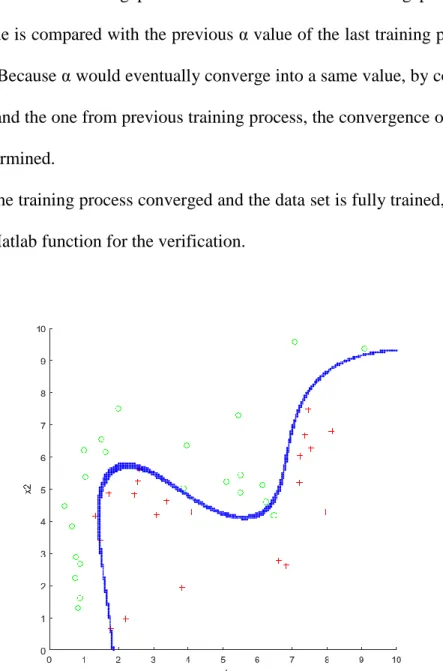
A sample is compared with all other samples to get α value, α is stored in the data storage for future training process. In the end of each training process for one sample, α value is compared with the previous α value of the last training process of the same sample. Because α would eventually converge into a same value, by comparing the current value and the one from previous training process, the convergence of the training process is determined.
After the training process converged and the data set is fully trained, α values are verified in a Matlab function for the verification.
26
With the data set of a two dimensions training model and its α values, the training result is shown in graphic as Figure 3.3. On the other hand, for the higher dimensions, a testing data set is required for the final training result.
3.1.2 Cascade SVM Unit Setup
Apart from the basic SVM, a cascade SVM is also implemented in the previous ASIC design, it has a significant speedup and energy reduction compared with a basic SVM. The cascade SVM module is developed based on the cascade SVM discussed in previous section; however, there are some changes in the structure thanks to the characteristic of hardware implementation.
Due to the benefit of hardware implementations and the training process of the cascade SVM, the number of all the SVM units is the same as the maximum number of SVM subsets in the first layer of a cascade SVM structure.
27
Figure 3.4 A cascade SVM structure
Figure 3.4 shows that every layer operates at a different time, and the next layer always has less SVM units compared with the previous layer. If a SVM unit is reusable, the numbers of SVM units required for a cascade SVM can be reduced, which saves the device usage in hardware.
With a reusable SVM unit developed, the previous structure of Figure 3.4 is modified as Figure 3.5. At first, four SVM units train the data sets from the corresponding data storage of each SVM unit. After all of the units are trained, only two SVM units are activated again, they not only read SVs from its own data storage, but they also read from the data storage from their combined partner. In the end, only one SVM unit is activated, and it trains all SVs from four data storage.
SVM SVM SVM SVM
SVM
SVM Cascade SVM
28
Figure 3.5 A reusable cascade SVM unit structure
As a result, a cascade SVM has the following structure: reusable SVM units, address mapping units, multilayer system bus and processing configuration.
In the cascade SVM implementation, after the address is generated from the address generator in a SVM unit in Figure 3.1, it is fed into a memory manage unit, which translates the address according to the current layer. Figure 3.6 shows how memory management units are used in the last layer.
Figure 3.6 Memory management units implementation
SVM SVM SVM SVM
First time combined
Second time combined
SVM
MEM MEM MEM MEM
MMU MMU MMU MMU
Addresses and Results
Data new α
29
The indexes of SVs are stored in the memory manage unit, which are produced from reusable SVM units after convergence. On the other hand, every reusable SVM unit in each layer has its own memory manage unit, it stores indexes after each convergence and provides the correct address for the next training.
To separate every layer, it also has a multilayer system bus. The multilayer system bus records the convergences from every reusable SVM unit. Aside from that, the processing configuration feeds the corresponding sample into activated SVM units.
With the cascade SVM design discussed as above, it provides a faster training process compared with the basic SVM in 3.1.1. These two structures serve as the base of this research and by implementing these two structures in the FPGA platform, the issues on the ASIC platform can be solved.
3.2 UART System Implementation
Due to limitations of the ASIC platform, it is difficult to expand the dimensions of a training model in a faster manner and the data storage limitation constraints the possibility of large models training.
In order to solve the limitations of the original implementation, the design of the SVM is migrated to the FPGA. As a result, a UART system implementation is proposed in the beginning.
30
3.2.1 Hardware Structure Overview
First, to implement the design in the FPGA, a UART communication is added between the host computer and the FPGA for communication purpose, and the main structure is modified for synthesizability difference in the FPGA. A host computer is the user interface to communicate with the FPGA board, it is able to load the data for training and receive the training result. On the other hand, the memory structure is changed from SRAM structure to Block RAM.
The universal asynchronous receiver/transmitter system, which is known as the UART system, is a common communication method between computer hardware devices for data transfer [32]. The UART system transfers data by bits in sequence according to the corresponding speed of bit transition for the receiver and the transmitter, which is called baud rate. With the same speed between the transmitter and the receiver, it is able to interpret the signal correctly.
Start
bit Bit 1 Bit 2 Bit 3 Bit 4 Bit 5 Bit 6 Bit 7 Bit 8 Bit 9
Stop bit 1
Stop bit 2
Figure 3.7 UART data frame
From Figure 3.7, the data frame of the UART transition process is shown, noted that it only transfers 8 bits data at a time. Because the data storage in this design is a 32
31
bits fixed point format, it requires four transmission processes to transmit one sample from the FPGA board to the host computer, the user interface, with UART communication. On top of that, for this design, its baud rate is set as 115200 Bd, which indicates the transfer speed of each bit. On the other hand, peripheral component interconnect express, PCIe, is also a common transmission method with a high transmission speed, which is 2.5 gigabits per second. However, it requires more hardware device and setup requirement. The UART communication only requires 43 slices of registers, while the PCIe requires 673 slices of registers, which would increase 64.4% of the device utilization.
Aside from the UART implementation, the data storage of the FPGA implementation is the Block RAM (BRAM) storage [33]. The BRAM is a configurable memory module provided by Xilinx FPGA. It is memory storage with its data length and storage size modifiable by the user.
Figure 3.8 Hardware structure in the FPGA with UART Board (Top module) Host Compute UART Communication SVM training module
Block RAM address
data address
32
The hardware structure is shown as Figure 3.8. Firstly, a data set of the training model is loaded in the BRAM, which is connected to the SVM training module. The amount of BRAMs is same as the number of SVM units, because every SVM unit has its own memory storage. The SVM training module is discussed in 3.1, both basic and cascade SVM structures can be served as the SVM training module here.
After the SVM training module reports the convergence of the training process, the top module disconnects the BRAM from SVM training module, and connects it to the UART communication. That is, it reconnects the address input and data output from the SVM module to the UART communication. The receiver in the UART communication is connected with the address port of a BRAM, while the transmitter is connected to the data output port of a BRAM. Therefore the final training results can be read from the FPGA to the host computer.
After opening the serial port, it is able to send the address in four eight bits unsigned integers according to the setup of UART, which is shown in Figure 3.7, and saves the corresponding data. The receiving data is also interpreted from four eight bits unsigned integers to its correct value, which is saved for the further verification.
In this research, it is implemented in the Xilinx Virtex-6 FPGA ML605 evaluation board. Upon this point with the basic structure of SVM, the device utilization of a cascade SVM is around 1% of the FPGA, which gives flexibilities of expanding the original design. On the other hand, because of that a basic SVM only has one SVM unit; the device utilization is smaller than a cascade SVM. For a two cores cascade SVM design, it requires 2187 slices registers while the total device has 301,440 slices registers.
33
More dimensions can be introduced for training. As a result, the two dimensions design is expended to an eight dimensions design.
3.2.2 Multiple Dimensional Implementations
In order to expend dimensions, more registers are added as data storage and multipliers are parallelized for different dimensions data computation, higher dimensional data are able to be read in the training process, which is shown in Figure 3.9; additional parts are highlighted compared with the original design in Figure 3.1.By parallelizing the whole design makes training the training models with different dimensions in one design possible as long as the dimensions are less than the maximum dimensions. By setting the unused dimensions inputs as 0, it trains data sets without any difference with a design of the exact dimensions setup.
34
Figure 3.9 An 8-dimension SVM unit.
The shape marks for the additional dimensions registers and multipliers compared with a two dimensions SVM.
By replacing the SVM module in Figure 3.8 with a multiple dimensional SVM unit in Figure 3.9, data sets over two dimensions is able to be trained in the FPGA. Figure 3.9 shows that it still shares a similar structure with a two dimensions SVM unit. To understand the overall device utilization, the distribution of a two dimensions SVM unit implementation for the device utilization is shown as Figure 3.10. Most parts of the device are contributed to the internal computation, while in the computation most of the device is used in the multipliers, it requires 650 slices registers, the lookup table for the
Y X1 X2 SVM Multiplier Multiplier Computation Lookup Table Address Generator α Multiplier Multiplier Multiplier Multiplier Multiplier Multiplier X3 X4 X5 X6 X7 X8 α
35
exponential control requires 110 slices registers, and the address generator requires 108 registers.
Figure 3.10 Slices registers of distribution for two dimensions SVM unit
The Figure 3.11 shows the area break down of the top module control, UART communication and the SVM module. Most parts of the device are used for the SVM module.
67.22% 11.38%
11.07%
10.34%
Slices Registers Distribution in a SVM Unit
Multipliers Lookup Table Address Generator Other Computations
36
Figure 3.11 Slices registers distribution a two dimensions basic SVM FPGA implementation
From Figure 3.12, it shows the trend of device utilization growth as the dimensions increase. The higher dimensions it has, the more device it uses.
49 43
986 1044
Top module control UART control SVM module Total
Slices Registers Ditribution of FPGA Implementation
37
Figure 3.12 Device utilization in different dimensions
Though it is able to train multiple dimensional training models with the FPGA implementation, due to the UART communication between the host computer and the FPGA, the limitation of huge data sets training still exists. The process of data training itself has been speeded up, while the transfer speed of UART is slow for large data sets training.
3.3 Memory Card System Implementation
To solve the transfer speed issue, a new system design is introduced as followed. A 2G memory card (the compact flash card, CF card) is introduced into the design; therefore it is able to obtain the data in a faster manner and increase the size of training models that it is able to train.
1051 1350 1665 2187 2673 3497 0 500 1000 1500 2000 2500 3000 3500 4000
2 dimensions 4 dimensions 8 dimensions Slices
Registers Single SVM
38
3.3.1 Hardware Structure Overview
In order to manipulate a CF card in an easy manner, the Microblaze system is introduced. A Microblaze system is a soft-core microprocessor for Xilinx FPGA, it is able to control and interact with those features embedded in the FPGA according to the user’s setup, including a CF card control [34]. The system bus between the Microblaze system and other functions is the Advanced eXtensible Interface, AXI [35]. It is an on-chip connection between functional blocks in the embedded system.
With the help of a Microblaze system, it is possible to interact with a CF card with straightforward instructions in C, compared with the implementation in Verilog of complex timing setup and signal exchange.
Figure 3.13 Hardware structure in the FPGA with the memory card
In Figure 3.13, a Microblaze system is used, which is connected with a CF card control and a BRAM. The BRAM here, compared with the previous design, is working
Microblaze (System control) System Bus CF Card (Memory Card) BRAM SVM Base System Top module
39
as a buffer rather than the data storage. In this design, the BRAM is a dual-port BRAM that one port connects to the internal system bus, which is accessed by the Microblaze system; the other port is set as an external port and connects the SVM module. The SVM module is separated from the base system in order to have a different clock from the Micorblaze; therefore its clock will not interact with other system structures in the base system.
Figure 3.14 A BRAM buffer
The Figure 3.14 shows an insight of the BRAM buffer. Because the SVM unit is indirectly connected with the base system, the start command and the convergence signal are also stored in the BRAM buffer. Therefore the data storage is modified compared with the previous design.
System Bus BRAM SVM Base System Address Data Enable Clock Reset Address Data Enable Clock Reset
40
Address Data Address Data
0 Y1 0 * 1 X1,1 1 Y1 : : : X1,1 8 X1,8 8 : 9 Y2 9 X1,8 10 X2,1 10 Y2 : : : X2,1 9×N α1 9×N : 9×N +1 α2 9×N +1 α1
Figure 3.15 Data storage change
The * place stores the communication signal, including numbers of data, start and reset signal and converge signal.
From Figure 3.15, the left side represents the previous data storage order. The data of a sample is stored as the following way, its classification and rest of the dimensions data. After the whole data set is stored, α values are stored as the same order with its corresponding sample. For the right side, to communicate with the base system, the data set for training and its training results are moved for one storage space. With the spare space, the number of whole data set is sent first, and the convergence signal is read after the SVM module finishes training. On the other hand, if it is needed to start the
41
training process again with a new data set, the spare place is also used to give a restart signal to start a new training process.
On the other hand, if it is a cascade SVM structure, the BRAM buffer is multiplied according to the cores of the cascade SVM. That is, if it is a two cores cascade SVM, it would have two BRAMs in the system; each core has its own buffer. The data set is firstly stored in the CF card, and it is written into the BRAM buffer via the Microblaze.
After a data set is trained by the external SVM module, it is read from the buffer and written into the CF card again. If the intended data set is bigger than the size of the buffer, the Microblaze system divides the original data set, trains certain data and saves those outcomes first.
Figure 3.16 Data division in the Microblaze control Microblaze Control
data BRAM buffers
42
In Figure 3.16, the original data set is divided in the corresponding size of BRAMs, and the index of a dividing point is saved for the next division. After the data set is converged, the Microblaze control scans SVs from first round of training and write to the buffer again, working as the cascade SVM. As a result, it is capable of training data sets with the size constraint from a CF card instead of the size of BRAMs. However, the dividing point is chosen in order regardless of the classifications, the subset may become difficult to train compared with the original data set.
Though the memory card implementation provides the benefit of training a large data set with bigger size than the BRAM storage, in order to save not only indexes of separating points shown in Figure 3.16 but it also has to save all the indexes of SVs from the previous training results, it requires additional storage to record indexes. Apart from that, because this process is inside the Microblaze system and implemented in software, it would reduce the execution efficiency.
Therefore to save as more time as possible, one way is to speedup the reading process from a CF card to BRAMs. A subset is read firstly and the computation process is started. The control system loads the data to another BRAM buffer during the training process, which works as a dual buffers system. After those data are trained, SVM is able to start another training process immediately without data loading. For the cascade SVM, in order to have dual buffers, each core has two BRAM buffers. Therefore, for a two cores cascade SVM, it has four BRAMs in the design instead of two.
In Figure 3.17, it depicts the overall training process; the data set is stored in a CF card from the host computer, and it is read from a CF card after training. The data set
43
is stored in a text file and all of the samples are in a 32 bit binary form. However, for the values in the training result, they are stored as integer numbers.
Figure 3.17 Data path
In this system the data transfer speed is no longer limited to UART system speed; it only needs to read a CF card from the computer to get training results. Furthermore, the data storage is no longer limited to the FPGA itself, it depends on the CF card memory size that user chooses.
3.3.2 Experimental Setup of the FPGA
In this section, a detailed FPGA setup is addressed for further results studies in section 4.3, which has experimental results for real world data sets.
In the setup of Microblaze system, apart from the Microblaze core and its cache, the system advanced configuration environment, system ACE, is attached to the system bus for a CF card control. The local memory size is set according to the Microblaze
Data.txt CF card Alpha.txt Microblaze BRAM1 SVM BRAM2
44
system control implementation. And BRAMs are added, the number of BRAMs is determined by the SVM module used.
After the Microblaze system is set up and generated, the SVM module is included in the top module of the base system. The SVM module connects to the BRAM buffers, which is connected to the external ports from BRAMs. While everything is connected, the design is exported to the software develop kit.
For the control system setup inside the Microblaze, a xilkernel is chosen. It provides an easy and straightforward manner to control a CF card. By choosing the xilfatfs configuration, the data control is implemented inside the Microblaze system.
Xilkernel is a small and robust kernel in the Xilinx FPGA, it is highly customized and used for the higher level implementations [36]. Xilfatfs is one of the features provided by xilkernel. It provides read and write functions to files stored on a CF card. It supports the file systems of file allocation tables, FAT, from FAT12, FAT16, to FAT32. With the help of xilkernel and xilfatfs, the design is implemented in the Microblaze system.
Before the training process, the maximum training size has to be assigned by the user according to the size of BRAMs set up in the previous process. And in the base system, a stopping point is included to provide a checking method to avoid the data set is impossible to converge caused by the data separation of Microblaze controller, it stops the current training process and move to the next data set. Because the Microblaze controller divides the data set according to the order stored in the memory card without checking classifications, not all subsets would be as easy to train as the original data set.
45
3.4 Memory Improvement and Comparison
In the previous ASIC implementation, the total cache size of whole design is 8kB, and it is divided to smaller private caches for the cascade SVM units. On the other hand, with a large number of built-in BRAMs in the FPGA, the storage of data grows to 1872 kB. As a result, for the FPGA version with UART communication, it is able to train a training model with a relative larger data set compared with the ASIC version. And with the CF card version, the data storage grows to 2 GB, which has a significant growth in the data amount of training.
However, if more dimensions data sets need to be handled, the storage will be smaller. For an N dimensions sample, it requires N+2 32 bits storage. Because not only does it have to store its N dimensions data, it also needs to store its classifications and α values. The detail storage method is explained in Figure 3.14. As a result, the relation between data size and dimensions is provided in Figure 3.18.
Figure 3.18 Possible data size in the built-in BRAMs 117000 78000 58500 46800 0 50000 100000 150000 0 2 4 6 8 10 Data size Dimensions
46
Though this is inevitable, with a 2 GB CF card involved, it is still able to train a large amount of data because the overall storage is about a thousand times larger than the size of internal BRAMs with the help of Microblaze. In the chosen 2GB CF card in this design, it requires 56.7 MB of storage for system files storage in order to become accessible for the Microblaze system; however, it is relatively small compared with 2 GB, which only occupied about 2.84% of the storage.
In this section, two hardware implementations on the FPGA are illustrated, and the implementation of both basic and cascade SVM units are explained. With the implementation of these structures, the following experiments in the next sections are conducted, which provides the insight of these implementations.
47
4. EXPERIMENTAL RESULTS
The SVM structure is designed in Verilog, and then it is generated by Xilinx Platform Studio. Afterward, the design is implemented through translating, mapping, placing and routing, and generating bitstream. In the end, it is configured to the Xilinx Virtex-6 FPGA ML605 evaluation board.
4.1 Runtime Comparison
The runtime comparison is based on a software SVM solution implemented in Matlab on an Intel core i5-3210M CPU in 2.5GHz. The FPGA implementation with the UART system has the maximum frequency of 112.752 MHz for a single SVM and 80.369 MHz for the cascade SVM, while the system with memory card has the maximum frequency in 104.976MHz for a single SVM and 72.844 MHz for the cascade SVM. The runtime starts from the beginning of the training process, after data are all loaded, and ends when the training process completes.
Apart from the timing analysis setup, to test the runtime with both FPGA implementations, three two dimensions artificial data sets are chosen and trained in the eight dimensions hardware structures. In order to verify the training results, these three artificial data sets are designed with a specific hyperplane, and each of which has 50, 100 and 200 samples. The training results are obtained by Matlab through UART communication in the UART version, and for the memory card version, results are saved
48
in the CF card. After training, results are verified in Matlab with the original data set and the separating plane is generated in graph; Figure 4.1 is one of the training results.
Figure 4.1 A training result for a training model using a data set with 100 samples in UART version of cascade SVM training
49
4.1.1 Hardware Speedup
From Figure 4.2, there is a big improvement in runtime between software and hardware implementations. The software solution has a significant higher runtime compared with the hardware version.
On the other hand, for the single and cascade SVM, the runtime difference is more and more significant as the samples grow. The more detailed runtime is provided in Table 4.2.
Figure 4.2 Runtime of 50, 100, 200 samples 0 5 10 15 20 25 50 100 200 Time (s) Numbers of samples Software SVM Basic SVM Cascade SVM
50
On the other hand, due to the similarity between training and classification process, the hardware can be also used for the classification process. Both of basic and cascade SVM use SVs from the original data set, therefore they have the same classification process. With a testing data set with 50 samples and the basic SVM classification, the classification time is shown in Table 4.1.
Training Data Set Number of SVs Time
50 samples 10 4.76 ms
100 samples 16 7.62 ms
200 samples 25 11.91 ms
Table 4.1 Comparison of classification time
From Table 4.1, it has shown the classification time is less than fifty microseconds, on the other hand, the training process requires hundreds of microseconds to train a data set. The classification process is faster than the training process unless the testing data set is significantly large than the data set.
4.1.2 Basic and Cascade SVM Comparison
Table 4.2 gives a detailed runtime of all the testing data sets from Figure 4.2. As discussed before, a big difference between the basic and cascade SVM has shown. From section 2.2, a great speedup is introduced by using the cascade SVM compared with a basic SVM. And take the data set with 200 samples for example; around 4.3x speedup of
51
a cascade SVM compared with a basic SVM, and it also enjoys a 23.5x speedup compared with software SVM.
numbers of samples 50 100 200
Software 5.078 s 9.694 s 19.184 s
Hardware
Basic SVM 0.148 s 0.353 s 3.527 s
Cascade SVM 0.094 s 0.289 s 0.815 s
Table 4.2 Training runtime comparison
Apart from that, if more cores are involved in the cascade SVM, the training data size of each layer will be reduced more. As a result, it is able to have a more significant speedup if more cores are implemented.
4.2 Non-artificial Data Sets Training and Execution Time Comparison
Because both of systems are using the same SVM module, there is no difference in accuracy of training results. From section 4.1, it shows the frequency difference between the UART implementation and memory card implementation, which causes the runtime difference during the training process. Apart from artificial data sets, the following data sets are also tested. In order to transfer the relatively large amount of data through UART in the Matlab interface, the transfer speed becomes longer than the training process. For example, it takes 13.8 minutes to transfer 200 samples in the
52
Matlab interface, while the training process takes less than five seconds. As data sets grow, the transmission time would become longer.
On the other hand, to verify the dual buffers system and avoid the overheat issue caused by dual-ports BRAMs setup, the maximum samples for a BRAM to hold is set as 100 samples. Every implementation has a different constraint on BRAM samples training due to different data paths and BRAM connections. If more BRAMs are required in the design, the maximum BRAM size is reduced because more long data paths are introduced. For a basic SVM without dual buffers, the maximum training data size with lowest overheat issue is 64kB, while for a cascade SVM with dual buffers, the size is reduced to 4kB. The results are obtained according to the following data sets. On the other hand, the different accuracy between the basic and cascade SVM are not only determined by the original data set division, but also effected by the Microblaze system division. These data sets will be discussed in each sub section, and this section is mainly focused on the execution time discussion between two kinds of hardware implementations.
4.2.1 Pima Indians Diabetes Data Set
The Pima Indians Diabetes data set is tested, which has 796 samples in 8 dimensions [37]. These data are collected from the Pima Indians heritage, with all the patients are female over 21 years old. Each sample has 8 dimensions and 1 classification; those dimensions are medical facts of the patient, including numbers of pregnancy, plasma glucose concentration, diastolic blood pressure, triceps skin fold thickness,
53
insulin, body mass index, diabetes pedigree function and age. With this data set, more facts of the diabetes are shown.
On the other hand, it is also a widely used data set in machine learning algorithms training. For example, a generalized discriminant analysis and a least square SVM are used in order to find a more accurate way to identify the diabetes by using this data set [38]. In this study, it also gives an overview of other training results of the Pima Indians Diabetes data set. With other 60 training results of other algorithms, most of the accuracies lie in a similar range, from 70% to 80%. And in that research, it is able to achieve 82.05% of accuracy. For the basic SVM, it has 74.74% of accuracy, and for cascade SVM, it has 73.70% of accuracy. From the training results, both of the training methods reach similar training results as shown.
4.2.2 Vertebral Column Data Set
The Vertebral Column data set is also tested, which has 248 samples in 6 dimensions [39]. This data set is a medical data set to classify patients into two categories of their health conditions: normal and abnormal, and its 6 dimensions have the following information: pelvic tilt, lumbar lordosis angle, sacral slope, pelvic radius and grade of spondylolisthesis. These data are based on the patients’ body movements to know the health status of joints and bones. With the information, the patient’s body structure is classified as normal or abnormal.
With this data set, a research of computer aided diagnosis systems is developed [40]. In that research, it used the following learning algorithms to train the data sets,