University of Texas at Tyler
Scholar Works at UT Tyler
Computer Science Theses
School of Technology (Computer Science &
Technology)
Fall 7-17-2013
Knowledge Extraction from Survey Data using
Neural Networks
Imran Ahmed Khan
Follow this and additional works at:
https://scholarworks.uttyler.edu/compsci_grad
Part of the
Computer Sciences Commons
This Thesis is brought to you for free and open access by the School of Technology (Computer Science & Technology) at Scholar Works at UT Tyler. It has been accepted for inclusion in Computer Science Theses by an authorized administrator of Scholar Works at UT Tyler. For more information, please [email protected].
Recommended Citation
Khan, Imran Ahmed, "Knowledge Extraction from Survey Data using Neural Networks" (2013).Computer Science Theses.Paper 1.
KNOWLEDGE EXTRACTION FROM SURVEY DATA USING
NEURAL NETWORKS
by
IMRAN AHMED KHAN
A thesis submitted in partial fulfillment
of the requirements for the degree of
Master of Science in Computer Science
Department of Computer Science
Arun Kulkarni, Ph.D., Committee Chair
College of Engineering and Computer Science
The University of Texas at Tyler
May 2013
The University of Texas at Tyler
Tyler, Texas
This is to certify that the Master’s thesis of
IMRAN AHMED KHAN
has been approved for the thesis requirements on
April 23rd, 2013
i
Table of Contents
List of Tables ... iv List of Figures ... v Abstract ... vi Chapter 1 - Introduction ... 11.1 Organization of the Thesis ... 4
Chapter 2 – Background ... 5
2.1 Likert-Type Items ... 7
2.2 Likert-Scale ... 7
2.3 Data Analysis Procedures ... 8
2.3.1 Analyzing Likert-Type Data ... 9
2.3.2 Analyzing Likert Scale Data ... 9
2.3.2.1 Measure of Central Tendency using the Mean Method ... 10
2.4 Artificial Neural Networks ... 12
2.4.1 Kohonen Learning ... 15
2.4.2 Competitive Learning ... 18
2.5 ANN Performance Measure ... 19
2.5.1 Error Matrix ... 19
2.5.2 Overall Accuracy ... 20
2.5.3 User’s Accuracy ... 20
2.5.4 Producer’s Accuracy ... 21
2.6 Rule Extraction Techniques ... 21
2.6.1 Rule Extraction from ANN having a Large Number of Features ... 21
ii
2.6.3 Rule Extraction from Discrete Data ... 22
2.6.4 Rule Extraction from Continuous and Discrete Data ... 24
2.6.5 Rule Extraction by Inducing Decision Tree from Trained Neural Network ... 25
2.6.6 Rule Extraction from Two-Layered Networks ... 26
2.7 Review of Prior Research ... 27
Chapter 3 – Methodology ... 29
3.1 Knowledge Extraction Process ... 30
3.1.1 Preprocessing – Data Cleaning and Transformation ... 31
3.1.2 Clustering of Data using the Kohonen Neural Network ... 32
3.1.3 Rules Extraction Process ... 33
3.1.3.1 Rules Extraction ... 36
3.1.3.2 Rules Pruning ... 39
Chapter 4 - Results and Discussion ... 42
4.1. MARSI Survey ... 43
4.1.1 Preprocessing – Data Cleaning and Transformation ... 46
4.1.2 Clustering of Data using the Kohonen Neural Network ... 46
4.1.3. Rule Extraction Process ... 49
4.1.3.1 Rules Extracted using Extended-CREA ... 49
4.1.3.2 Rules Extracted using C4.5 ... 50
4.2. Teacher Evaluation Survey ... 52
4.2.1 Preprocessing – Data Cleaning and Transformation ... 53
4.2.2 Clustering of Data using the Kohonen Neural Network ... 54
4.2.3 Rules Extraction Process ... 55
4.2.3.1 Rules Extracted using Extended-CREA ... 55
4.2.3.2 Rules Extracted using C4.5 ... 56
Chapter 5 - Conclusion and Future Work ... 59
iii
5.2 Future Work ... 60
References ... 61
iv
List of Tables
Table 1. Survey Results Analysis I ... 5
Table 2. Survey Results Analysis II ... 6
Table 3. Examples of Likert Scale Response Categories ... 6
Table 4. Five Likert-Type Questions with Four Options ... 7
Table 5. Five Likert-Scale Questions with Five Options ... 8
Table 6. Data Analysis Procedures for Likert-Type and Likert Scale Data ... 10
Table 7. Categories in MARSI ... 11
Table 8. Conjunctive Rule Extraction Algorithm (CREA) ... 27
Table 9. Subset Oracle ... 27
Table 10. Normalization of Responses ... 31
Table 11. Extended Version of Conjunctive Rule Extraction Algorithm ... 36
Table 12. Algorithm for Count Method ... 37
Table 13. Illustration of Extended-CREA... 38
Table 14. Redundant Feature ... 38
Table 15. Rules in Human Readable Form ... 39
Table 16. Algorithm to Create a Tree for Rules that has Common Conditions ... 40
Table 17. Algorithm to Traverse the Tree to Extract Merged Rules... 40
Table 18. Extracted Rules ... 41
Table 19. Merged Rules ... 41
Table 20. Normalization of Responses ... 46
Table 21. Comparison of Results by Different Classifiers ... 47
Table 22. Confusion Matrix/Error Matrix of KNN Classifier ... 47
Table 23. Confusion Matrix/Error Matrix of C4.5 Classifier ... 48
Table 24. Performance Measure of KNN and C4.5 Classifiers ... 48
Table 25. Comparison of Different Rule Extraction Techniques ... 52
Table 26. Normalization of Responses ... 54
Table 27. Results of KNN and C4.5 Classifiers ... 54
Table 28. Confusion Matrix/Error Matrix of C4.5 Classifier ... 54
v
List of Figures
Figure 1. Grouping of Data using Mean Method ... 12
Figure 2. Three Layer Artificial Neural Network ... 13
Figure 3. Linearly Separable Data Samples ... 14
Figure 4. An Illustration of Clustering using Unsupervised Learning ... 15
Figure 5. Two Layer Network with Kohonen Learning ... 18
Figure 6. Overall Process to Extract Knowledge from a Likert Scale Data Survey ... 30
Figure 7. Data Cleaning and Transformation ... 31
Figure 8. Conversion from XLS Format to CSV Format ... 32
Figure 9. Two Layered Kohonen Neural Network . ... 33
Figure 10. Flow Chart of Rule Extraction Process ... 35
Figure 11. Tree of Generated Rules ... 41
Figure 12. Screen Shot of Weka. Displaying the Properties Initialized for C4.5 Algorithm ... 43
Figure 13. MARSI Survey (Continued) ... 44
Figure 13. MARSI Survey ... 45
Figure 14. Performance Measure of KNN and C4.5 Classifiers ... 49
Figure 15. Teacher Evaluation Survey ... 53
vi
Abstract
KNOWLEDGE EXTRACTION FROM SURVEY DATA USING
NEURAL NETWORKS
IMRAN AHMED KHAN
Thesis Chair: Arun Kulkarni, Ph. D.
The University of Texas at Tyler
May 2013
Surveys are an important tool for researchers. Survey attributes are typically discrete data
measured on a Likert scale. Collected responses from the survey contain an enormous amount of
data. It is increasingly important to develop powerful means for clustering such data and
knowledge extraction that could help in decision-making. The process of clustering becomes
complex if the number of survey attributes is large. Another major issue in Likert-Scale data is
the uniqueness of tuples. A large number of unique tuples may result in a large number of
patterns and that may increase the complexity of the knowledge extraction process. Also, the
outcome from the knowledge extraction process may not be satisfactory. The main focus of this
research is to propose a method to solve the clustering problem of Likert-scale survey data and to
propose an efficient knowledge extraction methodology that can work even if the number of
unique patterns is large. The proposed method uses an unsupervised neural network for
vii
proposed to extract knowledge in the form of rules. In order to verify the effectiveness of the
proposed method, it is applied to two sets of Likert scale survey data, and results show that the
proposed method produces rule sets that are comprehensive and concise without affecting the
1
Chapter 1
Introduction
A survey is conducted to collect data from individuals to find out their behaviors, needs
and opinions towards a specific area of interest. Survey responses are then transformed into
usable information in order to improve or enhance that area. It is also referred to as a research
tool. It consists of a series of questions that a respondent has to answer in a specific format. The
respondent has to select among the options given to each question. Survey data attributes can
come in the forms of binary-valued (or binary-encoded), continuous data or discrete data
measured on a Likert scale. All three forms of data attributes are used according to the survey
requirements. Discrete data can be used as a measure on a Likert scale to provide some distinct
advantages over the other two types of data attributes. A Likert scale gives more options to
respondents as compared to a binary valued survey. A Likert scale also helps respondents choose
an answer. For instance, some respondents may be too impatient to make fine judgments and to
give their responses on a continuous scale. The options provided in a typical five-level Likert
item are Strongly Disagree, Disagree, neither Agree nor Disagree, Agree and Strongly Agree. The
collected data might be contaminated if the difficult or time consuming judgmental task is beyond
the respondent's ability or tolerance. The use of a Likert scale has been proposed to alleviate these
difficulties.
Extracting knowledge from survey data is a very important step in the decision-making
process. Based on this knowledge, decisions are taken to improve the area for which the survey
2
statistical methods available to perform analysis on survey data. A few of them are discussed in
the next chapter. These methods can perform basic to advanced response analysis. Some of the
methods are also effective to perform clustering of the survey data. Clustering is a process that
groups data into classes or categories based on the features or attributes of the data. The
partitioning of data is performed by a clustering algorithm without any explicit knowledge about
the groups. Clustering is useful where groups are unknown or previously unknown groups need to
be found [1]. Some clustering algorithms are discussed in the next chapter. Statistical methods
can cluster data, but in-depth knowledge cannot be extracted using these methods.
Clustering of Likert-scale survey data depends on the type of data and the number of
attributes. The process of clustering becomes more complex when the number of Likert scale
options and attributes in the survey is large. In the case of a survey, these attributes or features are
the questions. Another major issue in Likert-Scale data is the uniqueness of the tuples. Clustering
algorithms group data based on the patterns of the attributes. A large number of unique tuples
may result in a large number of patterns. Due to a large number of patterns, the knowledge
extraction process from these classifiers becomes complex, and often the outcome of knowledge
extraction process may not be satisfactory. The extracted information is usually expressed in the
form of if-then-else rules. These rules describe the extent to which a test pattern belongs or does
not belong to one of the classes in terms of antecedent and consequent. The main focus of this
research was to apply an unsupervised neural network to cluster Likert-scale survey data and to
propose an efficient knowledge extraction methodology that can work even if the number of
patterns is large.
There are many classifiers available such as an Artificial Neural Network (ANN) [2, 3, 4,
5], C4.5 [6] and ID3 [7] etc. An ANN is a powerful technique to solve many real world problems.
3
adapt themselves to changes in the environment. The basic architecture of an ANN consists of
three types of neuron layers: input, hidden, and output. An ANN is further divided into two
categories: supervised and unsupervised. In unsupervised learning, no class label information
exists, and the system forms groups on the basis of input patterns. An unsupervised neural
network adjusts itself with new input patterns. These input patterns are presented to the network
and it is supposed to detect the similarity in the input patterns. There are several unsupervised
neural networks, but the project has applied the Kohonen neural network due to its simple
architecture [8]. The Kohonen neural network is one of the simplest unsupervised networks that
consist of two layers. The first layer is the input layer, and the second layer is the Kohonen Layer.
Each unit in the input layer has a feed-forward connection to each neuron in the Kohonen layer.
The method proposed in this research consists of three steps. The first step is
preprocessing. In the preprocessing step, data cleaning techniques are applied on survey
responses and convert those responses into a network readable format. The second step is to apply
the Kohonen neural network to group data tuples into different clusters. The third step is to
extract knowledge from the neural network in the form of rules and optimize them to obtain a
comprehensive and concise set of rules.
The proposed method was applied to two Likert scale surveys. The first survey was about
the reading strategies of students. The name of the survey was “Metacognitive Awareness of
Reading Strategies Inventory (MARSI)” [9]. It has 30 questions, and each question has five
options. The second data set is a teacher evaluation survey. The teacher evaluation survey form
consisted of eight questions; each question had five options. It was used to evaluate a teacher’s
4
1.1
Organization of the Thesis
The chapters in this thesis are organized as follows. Chapter 2 reviewed the statistical
methods for analysis of Likert scale data. An artificial neural network is discussed along with
clustering algorithms. Various rule extraction techniques are also explained in the chapter.
Chapter 3 describes the proposed methodology and clustering using unsupervised neural
networks. It also explains the proposed rule extraction algorithm. Chapter 4 mainly illustrates the
results. The error matrix and other performance measures are discussed for each example. It also
compares the results of the proposed method with results of C4.5 classifier. Chapter 5 provides a
5
Chapter 2
Background
Survey responses contain an enormous amount of data, consisting of binary-valued or
binary-encoded data, continuous data, or discrete data measured on a Likert scale. Extracting
knowledge from survey data is a very important step in a decision-making process. Analyzing
results of a survey depend on the type of data and the number of attributes. The process of data
analysis becomes more complex when the number of questions and attributes in the survey is
large.
Statistical analysis of survey results is limited. It only describes the percentage for each
response. For example, a typical question on a binary survey would be “Do you own a
Smartphone?” and provided response options are “Yes” and “No”. An Analysis of this type of
survey would result in some kind of percentage of responses as described in Table 1 [10].
Table 1. Survey Results Analysis I
Value Percentage
Yes 87%
No 13%
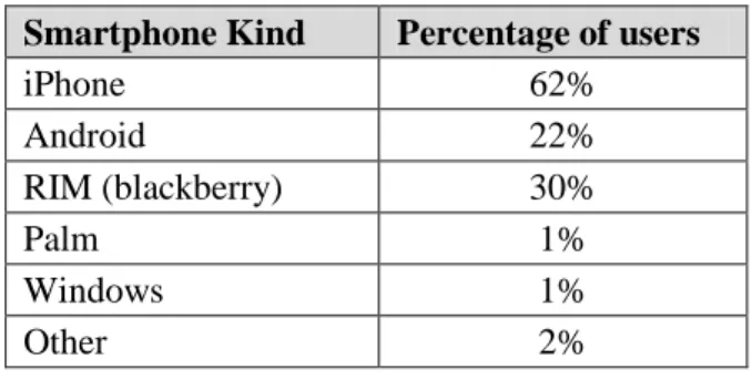
It is also common to analyze survey results by separating respondents into groups or
categories based on the gender or any other attribute. In this way, an analysis report may generate
results in a more detailed format. Taking the same example as above, it is possible to generate
6
Table 2. Survey Results Analysis II
Smartphone Kind Percentage of users
iPhone 62% Android 22% RIM (blackberry) 30% Palm 1% Windows 1% Other 2%
The above analysis can be helpful in a binary valued survey, but in the case of a Likert
scale survey, it will be a problem to organize results into a coherent and meaningful set of
findings. As in a Likert scale survey, the response of a person can vary between given options.
Generally, five options are provided for selection. Some examples of those options are shown in
Table 3.
Table 3. Examples of Likert Scale Response Categories
Scale 1 2 3 4 5
Never Seldom Sometimes Often Always
Strongly Agree Agree Neutral Disagree Strongly Disagree Most important Important Neutral Unimportant Not Important at all
Analysis of Likert scale survey data is a much more complex task as compared to a
binary valued survey due to the number of options for each question. Analyzing the Likert scale
survey data in the same way as a binary valued survey might show incorrect analysis results. One
mistake commonly made in analyzing this type of survey is the improper analysis of individual
questions on an attitudinal scale. Another important aspect in analyzing this type of survey is to
understand the difference between Likert-Type and Likert Scales [11]. Analysis procedures are
different for both Likert-Type and Likert Scale surveys. Basic concepts about Likert survey are
7
2.1 Likert-Type Items
The difference between type items and Likert scales is described in [12].
Likert-type items are identified as a single question that uses some aspect of the original Likert response
alternatives. While multiple questions may be used in a research instrument, there is no attempt
by the researcher to combine the responses from the items into a composite scale. Five samples
of Likert-Type questions are shown in Table 4. These questions have no center or neutral point,
so they cannot be combined into a single scalar value. A respondent has to choose whether they
agree or disagree with the question [12].
Table 4. Five Likert-Type Questions with Four Options
Strongly
Disagree Disagree Agree
Strongly Agree 1. I feel good about my work on
the job. SD D A SA
2. I am satisfied with job
benefits SD D A SA
3. My office environment is
friendly SD D A SA
4. I feel like I make a useful
contribution at work SD D A SA
5. I can start working on a
project with little or no help SD D A SA
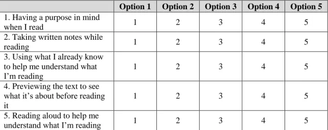
2.2 Likert-Scale
A Likert scale is composed of a series of four or more Likert-type items that are
combined into a single composite score/variable during the data analysis process [11]. These
Likert-type items may vary from one survey to another. An example of five Likert-scale
8 Option 1: I have never heard of this strategy before.
Option 2: I have heard of this strategy, but I don’t know what it means.
Option 3: I have heard of this strategy, and I think I know what it means.
Option 4: I know this strategy, and I can explain how and when to use it.
Option 5: I know this strategy quite well, and I often use it when I read.
Table 5. Five Likert-Scale Questions with Five Options
Option 1 Option 2 Option 3 Option 4 Option 5
1. Having a purpose in mind
when I read 1 2 3 4 5
2. Taking written notes while
reading 1 2 3 4 5
3. Using what I already know to help me understand what
I’m reading 1 2 3 4 5
4. Previewing the text to see what it’s about before reading it
1 2 3 4 5
5. Reading aloud to help me
understand what I’m reading 1 2 3 4 5
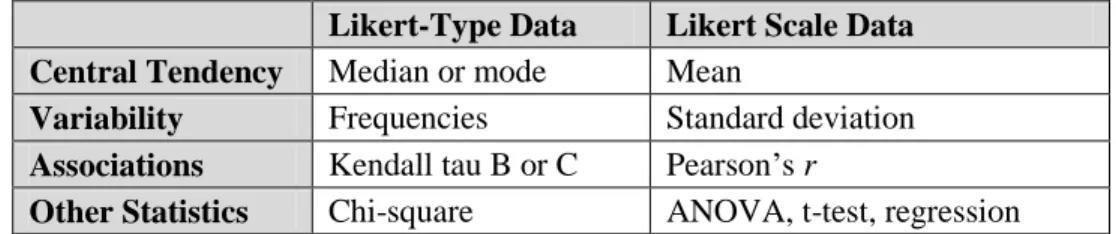
2.3 Data Analysis Procedures
Analyzing procedures for Likert Type data and Likert Scale data are different as shown in
Table 6. Four levels of measurements must be discussed in order to understand the data analysis
procedure. These four levels of measurements are also referred as a “Steven's Scale of
Measurement” [13].
A Nominal scale can be based on natural or artificial categories with no numerical
representation associated with it. Examples of nominal scale data include gender, name of a book
9
An ordinal scale refers to an order or rank such as ranking of students in a class,
achievement etc. With an ordinal scale, order or rank can be described, but the interval between
the two ranks or order cannot be measured.
An Interval scale shows the order of things and also reflects an equal interval between
points on the scale. Interval scales do not have an absolute zero. Measurement of temperature in
degrees Fahrenheit or Centigrade is an example of an interval scale.
A Ratio scale uses numbers to indicate order and reflects an equal interval between points
on the scale. A ratio scale has an absolute zero. Examples of ratio measures include age and years
of experience.
2.3.1 Analyzing Likert-Type Data
In Likert-type data, the interval between numeric values cannot be measured. A number
assigned to Likert-type items has a logical or ordered relationship to each other. The scale permits
the measurement of a degree of difference but not the specific amount of difference. Due to these
characteristics, Likert-type items fall into the ordinal measurement scale. Procedures to analyze
ordinal measurement scale items include median for central tendency, frequencies for variability,
and Kendal tau B or C procedure for associations [11].
2.3.2 Analyzing Likert Scale Data
Likert scale data have ordered and equal intervals. Numbers assigned to a Likert Scale
have an ordered relationship to each other. It also reflects an equal interval between the points on
the scale. Due to these characteristics, Likert Scale items fall into the interval measurement scale.
Procedures to analyze interval scale items include: arithmetic mean, standard deviation and
10
Table 6. Data Analysis Procedures for Likert-Type and Likert Scale Data
Likert-Type Data Likert Scale Data
Central Tendency Median or mode Mean
Variability Frequencies Standard deviation
Associations Kendall tau B or C Pearson’s r
Other Statistics Chi-square ANOVA, t-test, regression
2.3.2.1 Measure of Central Tendency using the Mean Method
Central tendency is a single value that attempts to describe a set of data by identifying the
central position within that set of data. The clusters formed by measuring central tendency are
based on the domain and the requirements of the survey. In this method, “mean” has been
measured for each section of the survey in order to interpret respondents’ answers to it. This
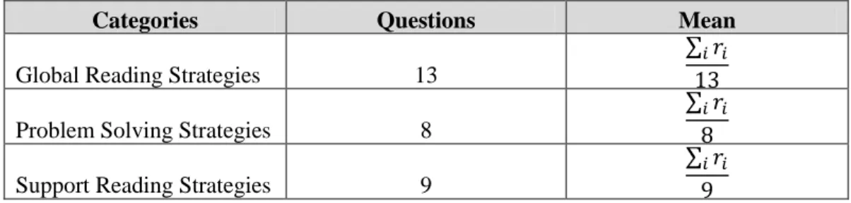
approach is demonstrated by using the MARSI survey. This survey has 30 questions and each
question has five-level Likert items. The MARSI survey consists of three sections: ‘Global
Reading Strategies’, ‘Problem Solving Strategies’ and ‘Support Reading Strategies’. Each answer
is interpreted on a 1 to 5 scale. The mean method is applied to the MARSI survey in the following
manner:
First, determine the number of questions in each section. This number will be used to determine
the mean for each section. It is recommended to calculate the mean for each section separately
[9]. Adding them together may result in an incorrect analysis. The number of questions in each
section of the MARSI survey is shown in Table 7.
Second, add responses r of each question in a section, and divide it by the total number of
questions in that section. In this case, for section ‘Global Reading Strategies’, the responses of
11
Table 7. Categories in MARSI
Categories Questions Mean
Global Reading Strategies 13
∑
Problem Solving Strategies 8
∑
Support Reading Strategies 9
∑
Third, add the means of all questions, and divide it by the total number of sections in the survey.
In this case, the total number of sections is 3. So, the mean of the three sections will be added and
then divided by 3. This will result in a single value.
Forth, the result of step 3 can be interpreted according to the requirements. In the case of MARSI,
if the value is 3.5 or higher, it will be considered as “High Level of Awareness”. If the value is 2.5 to 3.4, then it will be interpreted as “Medium Level of Awareness”. If the value is 2.4 or
lower, then it will be interpreted as “Low Level of Awareness”. This interpretation is strictly
based on the domain and the requirements of the survey.
Fifth, repeat steps 1 to 4 for each survey tuple.
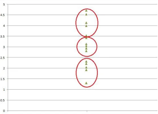
This method has been applied to the MARSI Survey and, for illustration purposes, fifteen
samples are plotted on a graph as shown in Figure 1. By using a graph, it can be seen how
measures of central tendency can act as an effective tool in clustering of the data. The graph
below shows the grouping of students, where three different circles indicate three different
clusters. Each cluster has 5 samples. The bottom group shows “Low Level of Awareness”. The middle Group shows “Medium Level of Awareness” group. The top group shows “High Level of Awareness”.
12
Figure 1. Grouping of Data using Mean Method
This method is effective for grouping, but users cannot extract patterns and trends
through which a sample falls into a group. This research has addressed this issue by using an
Artificial Neural Network (ANN). An ANN can be used for clustering data into different groups.
The ANN uses a rule generation technique to extract patterns and trends in order to justify any
decision reached.
2.4 Artificial Neural Networks
An Artificial Neural Network (ANN), usually called a neural network (NN), is a
mathematical or computational model that is inspired by biological neural networks. ANN
classifiers offer greater robustness, accuracy and fault tolerance. Neural networks are capable of
13
such as stocks estimation, remote sensing and pattern recognition. Studies comparing neural
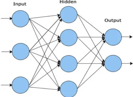
network classifiers and conventional classifiers are available [14]. An artificial neural network
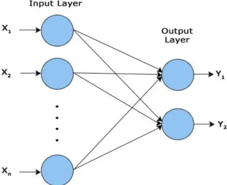
with three layers is shown in Figure 2. The first layer has input neurons which send data via
connection links to the second layer of neurons, and then via more connection links to the third
layer of output neurons. The number of neurons in the input layer is usually based on the number
of features in a data set. The second layer is also called the hidden layer. More complex systems
will have multiple hidden layers of neurons.
Figure 2. Three Layer Artificial Neural Network
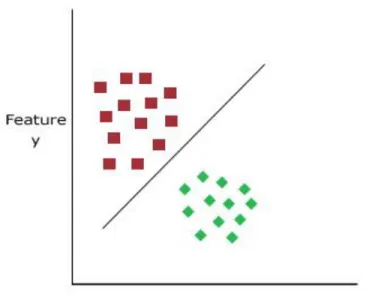
A network with only two layers can be applied to linearly separable problems. Linearly
separable problems are those where data samples can be separated by a single line as shown in
Figure 3. Data samples in Figure 3 are separated based on features x and y. Networks with one or
more hidden layers can be used to classify non-linearly separable data. The links between neurons
store parameters called "weights". The entire learning of a neural network is stored inside these
14
Figure 3. Linearly Separable Data Samples
.
Neural network classifiers can be used for a wide variety of problems. There are several
pattern recognition techniques used, but they are mainly categorized into two main categories,
supervised and unsupervised methods. In the case of supervised methods, a certain number of
training samples are available for each class. The neural network uses these samples for training.
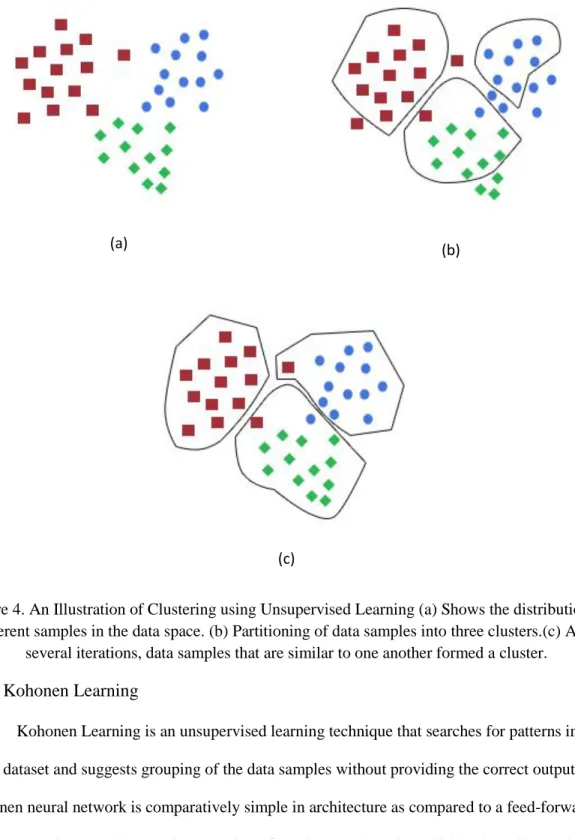
In an unsupervised method, no training samples are available. An illustration of clustering using
the unsupervised method is shown in Figure 4. Many well-defined algorithms are already
established for clustering using neural network models. Competitive learning and Kohonen’s
self-organizing maps are examples of unsupervised learning methods. In this research, Kohonen’s
15
(a) (b)
(c)
Figure 4. An Illustration of Clustering using Unsupervised Learning (a) Shows the distribution of different samples in the data space. (b) Partitioning of data samples into three clusters.(c) After
several iterations, data samples that are similar to one another formed a cluster.
2.4.1 Kohonen Learning
Kohonen Learning is an unsupervised learning technique that searches for patterns in a
given dataset and suggests grouping of the data samples without providing the correct output. A
Kohonen neural network is comparatively simple in architecture as compared to a feed-forward
back propagation neural network. It consists of two layers. There is no hidden layer in a Kohonen
16
The architecture for a Kohonen network is shown in Figure 5. Each unit in the input layer has a
feed-forward connection to each unit in the Kohonen layer. Units in the Kohonen layer compete
when an input vector is presented to the layer. Each unit computes the matching score of its
weight vector with the input vector. The unit with the highest matching score is declared the
winner. Only the winning unit is permitted to learn [15]. The learning algorithm is described
below.
First, initialize the elements of the weight matrix W to small random values. Element of
matrix W represents the connection strength for the connection between unit j of layer and unit i of layer . These random weights must be normalized before training starts. The weights can be normalized by multiplying the actual weight with a normalization factor. The normalization factor is the reciprocal of the square root of the vector length:
√
where VL is the vector length. Vector length can be calculated using Equation (2).
∑
where i represents the output class, and j represents the input unit.
For step 2, presentthe input vector x= (x1, x2… xn)
T
; the input to the network must be between the
values -1 and 1. A normalization factor should be calculated using input values as shown in
Equation (1). In this step, the input values will remain unchanged, but the normalization factor
17
For step 3, calculate the value for each output neuron by calculating the dot product of the input
vector and weight between the input neurons and output neurons.
∑( )
This output must now be normalized by multiplying it by the normalization factor that was
determined in step 2.
Now, this normalized output must be mapped to a bipolar number. A bipolar number is an
alternate way of representing binary numbers. In the bipolar system, binary zero maps to -1, and
binary 1 remains at 1. As the input was mapped to a bipolar number, similarly the output must be
mapped to a bipolar number. It can be accomplished by using Equation (5).
For step 4,after calculating the output value for each output neuron, a winner must be chosen.
The output unit having the largest output value will be chosen as the winner.
For step 5, the weights of the winning neuron are updated. The weights of a link between an
output neuron and an input neuron can be updated by using two methods: the additive method and the subtractive method.
The additive method uses Equation (6).
18 The subtractive method uses Equations (7) and (8),
where x is the training vector, k indicates the iteration number, and α is the learning rate. The
typical value of the learning rate ranges from 0.1 to 0.9. This research has used the subtractive
method.
For step 6, repeat steps 2 to 5 for all input samples.
Figure 5. Two Layer Network with Kohonen Learning
2.4.2 Competitive Learning
Malsburg [16] and Rumelhart and Ziper [17] have developed models with competitive
learning. It is called a competitive algorithm because units within each layer compete with one
19
an incoming pattern, the more it inhibits other units within the layer. Similar to Kohonen,
competitive learning uses normalized weights w and inputs x. The output value of each neuron is
calculated by Equation (9),
∑
where i is the output layer neuron, and jrepresents the input unit. The output unit with the
largest output value will be chosen as the winner. The weights of all links are updated using
Equation (10),
( )
where C represents the activation value of input neurons. If the input value is greater than the
normalization factor, then the input neuron will be considered as active. For active input neurons,
the value of C will be 1; otherwise, it will be 0. The variable n represents the total number of
active lines and. α represents the learning rate. A typical value of the learning rate ranges from
0.1 to 0.9.
2.5 ANN Performance Measure
There are various performance measures that can be evaluated in order to determine the
accuracy and performance of a classifier. These measures are used for assessing the prediction
accuracy of a classifier. This research has used the following performance measures to assess the
ANN model.
2.5.1 Error Matrix
An error matrix is also called the Confusion Matrix (CM). It is a useful tool for analyzing
20
represents the predicted class. However, each row represents the actual class. If represents an error matrix, then indicates the number of tuples of class i that were classified in class j. In the same manner, and indicate the correctly classified tuples of class i and j
respectively. To illustrate the comparison of an ANN classifier with other classifiers, an error
matrix has been evaluated.
2.5.2 Overall Accuracy
The overall accuracy is computed by dividing the total number of correctly classified
samples in all classes by the total number of samples,
∑
where represents overall accuracy, r is the number of rows in the matrix, is the number of classified samples in row i and column i , and N is the total number of samples.
2.5.3 User’s Accuracy
User’s Accuracy indicates the probability that a sample classified in a class actually belongs to that class. It is computed by dividing the total number of correctly classified samples
in a class with the total number of samples in that class (i.e., row total in error matrix),
where is the user’s accuracy of class i, is the number of samples in row i and column i, and
21
2.5.4 Producer’s Accuracy
Producer’s Accuracy indicates the probability of a reference sample being correctly classified. It is computed by dividing the total number of correctly classified samples in a
category with the total number of samples classified in that category by the classifier (i.e., column
total in error matrix).
where is the producer’s accuracy of class i, is the number of samples in row i and column i, and is the marginal total of column i in the error matrix.
2.6 Rule Extraction Techniques
The trained knowledge-based network is used for rule generation in if-then form in order
to justify any decision reached. These rules describe the extent to which a test pattern belongs or
does not belong to one of the classes in terms of antecedent and consequent clauses. There are
numerous methods to extract rules from an ANN. A few of them are described in the following
sections.
2.6.1 Rule Extraction from ANN having a Large Number of Features
Sometimes data that are used for classification contain a large number of attributes and
features. Having a large feature space may result in a large number of rules with a large number
of antecedents per rule. To overcome this issue, “Rule Extraction Artificial Neural Network
Algorithm (REANN)” has been proposed [18]. This algorithm proposed that pruning of the neural network will help in extracting more comprehensible and compact rules from the network.
Pruning is the process in which features are removed redundantly on the basis of relevance. It
22
Extraction (REx) algorithm is applied. REx is composed of three major functions: rule extraction,
rule clustering and rule pruning. The pruning function eliminates redundant rules by replacing a
specific rule with a more general one, and then removes noisy rules. The efficiency of this
method is better in terms of accuracy, number of rules and number of conditions in a rule, but the
REANN algorithm is only effective for data having a large number of features.
2.6.2 Rule Extraction from Binary Data
A dataset may often consist of binary data. For example, consider data collected from a
survey consisting of binary-valued attributes. Surveys with binary valued attributes are usually
less time-consuming. They also facilitate respondents to choose the answer from the given
Boolean options. To extract knowledge from a binary-valued survey data, a hybrid method has
been proposed [19]. This method has two components, an ANN and a decision tree classifier. The
network is trained and pruned using the technique utilized in REx algorithm. Then the decision
tree extracts rules from the trained network. This method is also proposed to use the M-of-N
construct [20] to describe the rules instead of “if-then-else” form. The M-of-N construct is mostly
suited for data with binary-valued attributes. The M-of-N construct expresses rules in a more
comprehensive way. It also reduces the number of rules. The proposed method is generally
effective, but it has some limitations as well. Survey data usually contain a large amount of
attributes and data that affect the training process of the neural network in terms of performance.
It also results in a large number of rules with many M-of-N constructs. This method is only
applicable to binary-valued survey data. The method also requires preprocessing of data when
some of the responses are not binary-valued.
2.6.3 Rule Extraction from Discrete Data
Sometimes a data set contains only discrete-valued attributes. To extract rules from such
23
algorithm searches for the best rule in terms of the number of samples it classifies, size of
subspaces it covers and the number of attributes in the rule. The algorithm consists of three steps.
First, it creates a rule set by adding one rule at a time for every input subspace defined by all the
combination of the input attribute values. In the second step, the merging process is applied.
Rules that classify sample data into the same category are merged into one classification rule. In
the third step, rules that cover the maximum number of samples, highest number of irrelevant
attributes and the largest subspace of the input are selected as the best rules. This algorithm can
be incorporated with other rule extraction techniques as well. The GRG algorithm produces rule
sets that are accurate and concise. The method is limited to discrete data only and cannot be
extended for continuous data. Also, the performance of this method may decrease with a large
number of attributes.
The GRG algorithm emphasizes on better accuracy, but rules extracted from the network
using this method might not meet the fidelity requirement. Fidelity is a criterion for assessing the
rule extraction method; it reflects how well the rules mimic the network. In order to maintain the
fidelity of the rules without affecting the accuracy, the LORE (LOcal Rule Extraction) method
has been proposed [22]. The LORE method also overcomes the limitation GRG enforces on the
number of attributes. This method can be applied to any number of features. It has mainly four
steps. In the first step, partial rules are extracted from each sample. A partial rule contains a
subset of features that are sufficient to classify the sample. In the second step, the merging
process is applied. The merging process of the LORE algorithm is different from the GRG
algorithm. The LORE algorithm uses a Reduced Ordered Decision Diagram (RODD) for merging
rules. The RODD is similar to a decision tree, but in the RODD, ordering is defined on features,
and every path in the diagram must traverse the nodes in exactly this order. In the third step,
24
produces a set of rules that are accurate and concise. This method is generally effective, but it has
some limitations as well. The LORE method uses the RODD for merging operations. The RODD
is highly dependent on feature ordering. Bad feature ordering may result in large decision
diagrams, and this increases the computational complexity.
2.6.4 Rule Extraction from Continuous and Discrete Data
Sometimes data sets may contain both continuous and discrete-valued attributes. For
example, surveys contain both continuous and discrete-valued attributes. To extract knowledge
from such type of data, a new algorithm “TREPAN” has been proposed [23]. There are some similarities between the TREPAN and conventional decision tree algorithms such as CART [24]
and C4.5. TREPAN and these other algorithms learn directly from the training set. The
difference is that TREPAN interacts with the trained neural network along with the training set in
order to extract the decision tree. The TREPAN method is scalable and has the capability to
analyze binary data as well. The TREPAN method does not enforce any limitation on the number
of attributes; it can be applied to datasets having a large feature space.
Another algorithm “CRED” (a continuous/discrete Rule extraction via a decision tree induction) [25] has been proposed to extract knowledge from data having both continuous and
discrete-valued attributes. The difference between this method and TREPAN is the process to
build the decision tree. The CRED builds a decision tree based on the activation patterns of
hidden-output units and input-hidden units. However, TREPAN builds a decision tree based on
activation patterns of input and output units. The proposed method is not limited to just binary
data as described in previous sections. It has the capability to process binary, continuous and
discrete-valued attributes. The CRED algorithm also uses a hybrid approach. The network is
trained and pruned using the technique utilized in the REx algorithm. Decision trees are then
25
method is effective and gives better accuracy than C4.5 algorithm. A disadvantage is that the
CRED is not effective for networks with no hidden layer.
2.6.5 Rule Extraction by Inducing Decision Tree from Trained Neural Network
A decision tree built from the neural network can be used to extract rules. One method is
to extract a decision tree using the activation patterns of the input and output units using training
data and the given neural network [23]. Another method uses activation patterns of hidden-output
units and input-hidden units to build the decision tree [25]. Both of these methods are suitable for
discrete and continuous variables. Commonly used decision tree methods are ID3 and C4.5. C4.5
is a descendant of the ID3 algorithm. ID3 selects an attribute based on a property called
information gain. The one with the highest information gain is selected as an attribute. Gain
measure describes how well a given attribute separates the training sample into a targeted class.
Information gain can be calculated using Equation (15). Entropy must be calculated first in order
to measure the gain of an attribute. Entropy can be calculated using Equation (14). Entropy
measures the amount of information in an attribute. The range of entropy is “0” (perfectly
classified) to “1” (totally random),
∑
where :
is the set of samples.
is the set of classes in
is the entropy of set
26
∑
where:
is the information gain on set split on attribute
is Entropy of set
is the subsets created from splitting set by attribute such that ⋃ is the proportion of the number of element in to the number of elements in set
is Entropy of subset
2.6.6 Rule Extraction from Two-Layered Networks
Algorithms discussed above can only be applied to multi-layer networks where one or
more hidden layer(s) were used. The Kohonen neural network used in this research consists of
only two layers: the input and output layer. The Conjunctive Rule Extraction algorithm (CREA)
[26] has been introduced to extract rules from this kind of network. The CREA can also be
applied to multi-layered neural networks. This algorithm uses two different oracles that answer
queries about the knowledge being learned. The conjunctive rule extraction algorithm is outlined
in Table 8. The EXAMPLES returns the data tuples, It can be generated randomly or can return
the data tuples from the training set. In this research, EXAMPLES simply returned the training
set. The SUBSET oracle ascertains that the subset of the original rule agrees with the network or
not. An algorithm of method SUBSET is outlined in Table 9. CREA first forms a conjunctive rule
by including all the features of the sample provided by the EXAMPLES oracle. This original rule
is then generalized by dropping one feature at a time and generating a subset of the original rule.
The SUBSET oracle returns true if this subset still agrees with the trained network. Otherwise, it
27
Table 8. Conjunctive Rule Extraction Algorithm (CREA)
/* initialize rules for each class */ for each class c
:= 0 repeat
e := EXAMPLES () c := Classify(e)
if e not covered by then
r := conjunctive rule formed from e
:= r
for each antecedent of r
r' := r but with dropped if SUBSET(c,r') = true then r:=r' := V
until stopping criterion met
Table 9. Subset Oracle
/* Test Subset whether it agrees with network or not */ fun SUBSET (c, ) := Classify( ) if c return true else return false
2.7 Review of Prior Research
There are various ways to extract knowledge from data. A number of previously
published papers on knowledge extraction using an ANN used either supervised or unsupervised
neural networks. Extraction of if-then rules from an ANN is the essential part of knowledge
discovery. Many articles that deal with the application of these knowledge extraction algorithms
have been published; a few of them are presented in the following paragraphs.
Kulkarni & McCaslin [27] proposed a method using artificial neural networks to extract
knowledge from multispectral satellite images obtained from a Landsat Thematic Mapper sensor.
28
models have been used to classify pixels in a multispectral image into three classes, water, land
and forest and to generate if-then rules. Jiang et al. [28] applied neural networks to medical
imaging problems. They analyzed, processed and characterized medical images using neural
networks. Panda et al. [29] described an application of artificial neural networks to estimate lake
water quality using satellite imagery. They proposed an indirect method of determining the
concentrations of chlorophyll-a and suspended matter, two optically active parameters of lake
water quality. This application has a potential to make the process of determining water quality
cost-effective, quick and feasible. Chan & Jian [30] developed a knowledge discovery system to
identify significant factors for air pollution levels using neural networks. Chen et al. [31] applied
the neural network system to predict fraud litigation for assisting accountants in developing audit
strategy. The results show that neural networks provide promising accuracy in predicting. They
proposed that an artificial intelligence technique is effective in identifying a fraud-lawsuit
29
Chapter 3
Methodology
The previous chapters have discussed how statistical methods can be used to analyze
Likert scale data. Clustering of data into different groups can be done effectively through these
statistical methods, but these methods do not describe “why” a data sample belongs to a particular
group. In this research, a method has been proposed that will resolve this issue by using the
Kohonen neural network for clustering. A Kohonen neural network learns by observation and
forms clusters of similar data samples. By using a Kohonen neural network, knowledge can be
extracted in the form of rules that explain the reason why the network made the decision to group
a data sample into a particular cluster.
The method proposed in this thesis to extract knowledge from Likert scale survey data
and group them into different clusters consists of three steps. The first step is preprocessing. In
the preprocessing step, data cleaning techniques are applied on survey responses before
converting them into a network readable format. The second step is to apply the Kohonen neural
network to group data tuples into different clusters. The third step is to extract knowledge from a
trained neural network in the form of rules and optimize those rules to obtain a comprehensive
and concise set of rules. The optimization of rules includes removing redundant rules, replacing
specific rules with more general rules and merging of rules. The overall process is shown in
30
Figure 6. Overall Process to Extract Knowledge from a Likert Scale Data Survey
3.1 Knowledge Extraction Process
Responses of surveys are provided in the XLS format (Microsoft Excel). The data is then
processed through different steps in order to obtain meaningful results. An application has been
built in C#.NET to implement these steps. The proposed method consists of the following steps,
31
3.1.1 Preprocessing – Data Cleaning and Transformation
The responses of the survey were provided in XLS format (Microsoft Excel). These
responses were then transformed to the format readable by the neural network. The overall
process is shown in Figure 7.
Figure 7: Data Cleaning and Transformation
In the first step, invalid responses must be removed. Invalid responses include questions that are
unanswered or answered outside of the given scale. Secondly, personal details must be
removed from the data set. Sometime surveys require respondents to enter their personal
information such as their ID, name, age, gender and ethnicity etc. These inputs were ignored
during conversion as they are not used for analysis. Normalization process is then applied to these
data tuples. A Kohonen neural network requires that the input be normalized to the range of -1
and 1. The mapping shown in Table 10 was used.
Table 10. Normalization of Responses
Option Option Value Normalized Value
Option 1 1 -0.9
Option 2 2 -0.4
Option 3 3 -0.1
Option 4 4 0.4
32
The results of the survey were provided in XLS format. The current implementation of the neural
network allows only comma separated values. To make neural network data readable, the data
must be converted into a CSV (comma separated values) file format. Conversion of a single
tuple from the XLS format to the CSV format is illustrated using Figure 8.
Figure 8. Conversion from XLS Format to CSV Format.
3.1.2 Clustering of Data using the Kohonen Neural Network
For clustering, a Kohonen neural network was used. It is an unsupervised learning
technique that searches for patterns in a given dataset and suggests grouping of input data
samples. The Kohonen neural network is comparatively simple in architecture as compared to a
back propagation neural network. It consists of two layers: the input layer and output layer. Due
to its simplicity, the network can be trained rapidly. It is also easier to extract rules from such
networks. The algorithm of Kohonen neural networks was discussed in detail in Chapter 2. A
Kohonen neural network with 30 neurons in the input layer and 3 neurons in the output layer is
33
Figure 9. Two Layered Kohonen Neural Network
3.1.3 Rules Extraction Process
Rule extraction algorithms are used for interpreting neural networks and mining the
relationship between input and output variables in the data. These rules are usually in the form of
“if-then-else” statements. They can also be referred to as extracted knowledge from the neural network. The rule extraction process used in this research consists of two steps: rule extraction
and rule pruning. Figure 10 illustrates the process to extract and reduce the number of rules. To
prioritize the rules beforehand, class-based ordering has been used as the rule ordering scheme. In
class-based ordering, classes were sorted in decreasing order of prevalence [1]. The class that was
34
I.
Rule Extraction:The extended version of the Conjunctive Rule Extraction Algorithm (CREA) has been
proposed to extract rules. This algorithm is discussed in the next section.
II.
Rule Pruning:Rule pruning includes removing redundant rules, replacing specific rules with more
general rules, and merging of rules.
Determining the default rule is another important aspect of the rule extraction process.
The default rule is evaluated when no other rule covers the sample. For different data sets, a
different default rule has been selected based on the number of samples classified in a class. The
35
36
3.1.3.1 Rules Extraction
Our approach extends the Conjunctive Rule Extraction Algorithm (CREA) discussed in
Chapter 2. This algorithm produces rules in an “if-then” format. The problem with Likert scale
data is its uniqueness and large number of attributes. If only CREA is applied, then it will result
in a large number of rules. It will treat each response separately and, due to the uniqueness in the
data tuples, a very small number of rules may be repeated. To overcome this problem, a heuristic
approach has been used in conjunction with the CREA algorithm. Instead of treating each
response separately, the proposed method calculates the count of each option in a rule generated
by the CREA method. The proposed algorithm for extracting rules from trained neural networks
is outlined in Table 11. Algorithm of the COUNT_METHOD is outlined in Table 12.
Table 11. Extended Version of Conjunctive Rule Extraction Algorithm
/* initialize rules for each class */ for each class c
:= 0 repeat
e := Examples() c := Classify(e)
if e not covered by then
r := conjunctive rule formed from e
:= r
for each antecedent of r
r' := r but with dropped if Subset(c,r') = true then r:=r' /* Apply count method */
:= COUNT_METHOD(r, )
:= V
37
Table 12. Algorithm for Count Method
fun COUNT_METHOD(r, ) := null
for all List of possible responses for all condition r
if value-part( ) = then = + 1 end if
end for end for
for all List of possible responses for all condition
if value-part( ) = then = + 1 end if
end for end for
for all List of possible responses if > 0 then if > then := V OptionName( ) '>=' else := V OptionName( ) '=' end if end if end for return
The COUNT_METHOD counts the number of occurrences of each option in a rule
generated by the CREA method and forms a new rule. This is accomplished by calculating the
number of occurrences of each option in the rule and compares it with the original rule. An
original rule consists of all the attributes and their values in a given sample. COUNT_METHOD
is effective in this case because survey attributes are of the same type and share the same set of
values. Applying this method to a data set with different types of attributes may result in incorrect
38
Table 13. Illustration of Extended-CREA
Assumptions:
1. There are a total five questions in the survey.
2. Five options are given with each question. i.e. OPT1, OPT2, OPT3, OPT4 and OPT5. 3. Responses of a single respondent are
For Question 1: selected → OPT4 For Question 2: selected → OPT2 For Question 3: selected → OPT5 For Question 4: selected → OPT2 For Question 5: selected → OPT3 4. Kohonen neural network grouped this tuple in cluster X.
In the first step, the Extended-CREA will form a conjunctive rule that will consist of all the
attributes (Equation 16).
If Q1=OPT4 and Q2=OPT2 and Q3=OPT5 and Q4=OPT2 and Q5=OPT3 Then Class X (16)
This original rule is then generalized by dropping one feature at a time and generating a subset of
the original rule. This will help to observe if responses to that feature are redundant. In this case,
“Question 1” will be dropped in the first iteration (Table 14).
Table 14. Redundant Feature
Question 2 → OPT2 Question 3 → OPT5 Question 4 → OPT2 Question 5 → OPT3
If this subset is classified as cluster X, then the dropped feature will be removed from the original
rule and considered as redundant information. If this subset is not classified as cluster X, then this
feature will remain part of the original rule. This process will be repeated for each antecedent.
Suppose after all iterations, the rule shown in Equation (17) is extracted.
39
By looking at this rule, it can be stated that the features Q1, Q3 and Q5 contain redundant
information, and the sample can be grouped in cluster X by using features Q2 and Q4.
COUNT_METHOD, being a heuristic approach, is finally applied to this extracted rule, which
transforms this rule as:
If C_OPT2 = 2 Then Class X (18)
where C_OPT2 represents the count of OPT2 in the extracted rule. This rule can be expressed in
human readable form (Table 15).
Table 15. Rules in Human Readable Form
If OPT2 is selected twice by the respondent Then Class X OR
If in two out of five questions respondent selected OPT2 Then Class X
3.1.3.2 Rules Pruning
The rules pruning process consists of three steps: remove redundant rules, replace specific
rules with more general ones, and merge rules. The merging of rules consists of two steps: create
a tree for rules that has common conditions, and traverse that tree to extract merged rules.
Algorithm to create a tree is outlined in Table 16 and algorithm to traverse the tree to extract
40
Table 16. Algorithm to Create a Tree for Rules that has Common Conditions
1. Repeat the following steps for each class. 2. Pull all rules for the current class.
3. Go through each rule in and count the number of occurrences of each condition in a rule.
4. Pick the highest occurred condition and create a root node of . Remove
from all rules. Add in vector . [
5. Pull the set of rules from that fulfill condition(s) in . Find the next highest
occurring condition in . If all conditions occurred once, then go to step 8.
6. Create node of from . Remove from . Add in vector .
[
7. Repeat step 5 and 6 until there is no condition in that occurred more than once. 8. Create nodes of all conditions in from . Remove all these conditions
from . Remove the last from vector . Repeat steps 5 to 8 until is empty.
9.
Remove rules from
that are already used.10. Repeat steps 2 to 9 for the rest of the rules until become empty.
Table 17. Algorithm to Traverse the Tree to Extract Merged Rules
1. Bottom-up, breadth-first traversing has been used.
2. Enqueue in Queue Q. Get the parent node of . 3. Enqueuenodes to Q until ≠ .
4. Dequeue all nodes from Q and combine those by using “OR”. Remove these nodes from
5. Create node of this combined condition from
6. Repeat steps 2 to 5 until all parent node nodes have only one child. This child must not be a parent of any node.
7. Traverse again in bottom-up, breadth-first order.
8. Merge child to its parent. If this child is not a parent of any child and there is no other sibling of this child, combine parent and child by using “AND”. Add this combine node to . . Remove and .
9. Repeat step 2 through 8 until tree-depth reduces to 1.
10. Extract the rule for each child node by combining it with using “AND”.
The merging process can be illustrated using the following example:
Suppose the following rules are extracted for class X using Extended-CREA. To make this
example simple, the consequent clause is not included as all the rules belong to the same class
41
Table 18. Extracted Rules
Rule 1: C_OPT3=5 C_OPT4=5 C_OPT5=8 Rule 2: C_OPT3=3 C_OPT4=4 C_OPT5=8 Rule 3: C_OPT4=7 C_OPT5=8
Rule 4: C_OPT2=5 C_OPT3=7 C_OPT4=4 C_OPT5=8 Rule 5: C_OPT3=6 C_OPT4=4 C_OPT5=8
Rule 6: C_OPT2=3 C_OPT3=6 C_OPT4=5 C_OPT5=8
The following tree is generated for these six rules using the above algorithm:
Figure 11. Tree of Generated Rules
This tree will be traversed to obtain following merged rules (Table 19):
Table 19. Merged Rules
Rule 1: C_OPT5=8 AND C_OPT4=7
Rule 2: C_OPT5=8 AND (C_OPT4=5 AND ((C_OPT2=3 AND C_OPT3=6) OR C_OPT3=5)) Rule 3: C_OPT5=8 AND (C_OPT4=4 AND ((C_OPT2=5 AND C_OPT3=7) OR C_OPT3=6 OR C_OPT3=3))
42
Chapter 4
Results and Discussion
As an illustration, this research has applied the proposed method to two different survey
data sets. The first survey is about reading strategies for students, and the second survey is
regarding teacher evaluation. To compare the efficiency of this proposed method, C4.5 has been
applied to the same datasets. The outcome of C4.5 is then compared to the results of the proposed
method. The C4.5 was applied using the open source software package Weka [32]. It is a
collection of machine learning algorithms for data mining implemented in Java. The C4.5
classifier was tested with a confidence factor of 0.25. The number of minimum instances per node
(minNumObj) was held at 2, and cross validation folds for the testing set (crossValidationFolds)
was held at 10 as shown in Figure 12. The confidence factor is used for pruning cross validation.
It splits the data set into a training set and a validation set. The algorithm trains using the new
43
Figure 12. Screen Shot of Weka. Displaying the Properties Initialized for C4.5 Algorithm
4.1. MARSI Survey
MARSI stands for “Metacognitive Awareness of Reading Strategies Inventory” [9]. It
was developed to assess a student’s reading awareness. It has 30 questions, and each question has
five-level Likert options. These 30 questions described 30 strategies or actions readers use when
reading book chapters, articles etc. This survey is divided into three sections: Global Reading
Strategies, Problem Solving Strategies and Support Reading Strategies. The ‘Global Reading
Strategies’ section contains 13 questions, the ‘Problem Solving Strategies’ section contains 8
44
45
46
This survey was conducted in December, 2011. The respondents were 6, 7 and 8th
graders. A total of 877 students participated in this survey. Most of the students were from ages
11 to 14. 344 students from 6th grade, 263 students from 7th grade, and 270 students from 8th
grade participated in the survey. The proposed method has been applied to MARSI survey data in
the following manner.
4.1.1 Preprocessing – Data Cleaning and Transformation
The responses of MARSI survey were provided in XLS format (Microsoft Excel). In this
step, responses were normalized to the range of 1 to -1. Normalization of the responses is given in
Table 20. After data cleaning, 860 records were selected for analysis. After normalization and
data cleaning, this file was converted to the CSV format.
Table 20. Normalization of Responses
Survey Option Short Form Option Value Normalized Value
I have never heard of this strategy
before. OPT1 1 -0.9
I have heard of this strategy, but I
don’t know what it means. OPT2 2 -0.4
I have heard of this strategy, and I
think I know what it means. OPT3 3 -0.1
I know this strategy, and I can
explain how and when to use it. OPT4 4 0.4
I know this strategy quite well,
and I often use it when I read. OPT5 5 0.9
4.1.2 Clustering of Data using the Kohonen Neural Network
A total of 860 samples were chosen for clustering. The “Mean” method was used initially
for clustering the MARSI survey data. It grouped the data into three clusters: “High Level of
Awareness”, “Medium Level of Awareness” and “Low Level of Awareness”. As the “Mean” method was used for clustering the MARSI survey data, its results were taken as the desired
47
information as it learns by observation. It grouped similar objects to form a cluster. In this
example, clustering results of the Kohonen neural network were compared with the “Mean”
method and C4.5 algorithm to measure the performance accuracy of the neural network.
The “Mean” method classified 607 samples in class 1, 235 samples in class 2 and 22
samples in class 3. The Kohonen neural network clustered 584 samples in class 1, 16 samples in
class 2, and 80 samples in class 3. A comparison of results by different classifiers is shown in
Table 21.
Table 21. Comparison of Results by Different Classifiers
Method Class 1 High Level of Awareness Class 2 Medium Level of Awareness Class 3 Low Level of Awareness Mean Method 607 231 22 KNN 584 196 80 C 4.5 627 220 13
The Error matrix of the KNN classifier and C4.5 are shown in Table 22 and Table 23
respectively. ”High Level of Awareness”, “Medium Level of Awareness” and “Low Level of
Awareness” represents clusters. Columns represent the predicted class while the rows represent the actual class. The recognition column represents the user’s accuracy.
Table 22. Confusion Matrix/Error Matrix of KNN Classifier
High Level of Awareness Medium Level of Awareness Low Level of Awareness Total Recognition High Level of Awareness 556 7 44 607 91.5% Medium Level of Awareness 28 167 36 231 72.3% Low Level of Awareness 0 22 0 22 0% Total 584 196 80 860 84.06%
48
KNN classified 91% samples correctly in class “High Level of Awareness”, 72.3% of
samples in class “Medium Level of Awareness” and none were classified correctly in class “Low Level of Awareness”. The reason class 3 had poor accuracy might be the small number of data samples in class 3.
Table 23. Confusion Matrix/Error Matrix of C4.5 Classifier
High Level of Awareness Medium Level of Awareness Low Level of Awareness Total Recognition High Level of Awareness 528 78 1 607 86.9% Medium Level of Awareness 97 129 5 231 55.8% Low Level of Awareness 2 13 7 22 31.8% Total 627 220 13 860 77.21%
A comparison of overall accuracy of different classifiers on