SAS 9.3 ODS Graphics. Getting Started with Business and Statistical Graphics. SAS Documentation

(1)

SAS

®

9.3 ODS Graphics

Getting Started with Business and

Statistical Graphics

(2)

The correct bibliographic citation for this manual is as follows: SAS Institute Inc. 2011. SAS® 9.3 ODS Graphics: Getting Started with Business

and Statistical Graphics. Cary, NC: SAS Institute Inc.

For a hardcopy book: No part of this publication may be reproduced, stored in a retrieval system, or transmitted, in any form or by any means, electronic, mechanical, photocopying, or otherwise, without the prior written permission of the publisher, SAS Institute Inc.

For a Web download or e-book: Your use of this publication shall be governed by the terms established by the vendor at the time you acquire this publication.

The scanning, uploading, and distribution of this book via the Internet or any other means without the permission of the publisher is illegal and punishable by law. Please purchase only authorized electronic editions and do not participate in or encourage electronic piracy of copyrighted materials. Your support of others' rights is appreciated.

U.S. Government Restricted Rights Notice: Use, duplication, or disclosure of this software and related documentation by the U.S. government is subject to the Agreement with SAS Institute and the restrictions set forth in FAR 52.227–19, Commercial Computer Software-Restricted Rights (June 1987).

SAS Institute Inc., SAS Campus Drive, Cary, North Carolina 27513. 1st electronic book, July 2011

SAS®_{Publishing provides a complete selection of books and electronic products to help customers use SAS software to its fullest potential. For} more information about our e-books, e-learning products, CDs, and hard-copy books, visit the SAS Publishing Web site at

support.sas.com/publishing or call 1-800-727-3228.

SAS®_{and all other SAS Institute Inc. product or service names are registered trademarks or trademarks of SAS Institute Inc. in the USA and other} countries. ® indicates USA registration.

(3)

Chapter 1

Introduction to ODS Graphics

What is ODS Graphics? . . . 1

SAS/GRAPH Output versus ODS Graphics . . . 2

The Suite of ODS Graphics Software . . . 2

Benefits of Using ODS Graphics Software . . . 3

Overview of ODS Destinations . . . 4

Components of a Graph . . . 5

What is ODS Graphics?

SAS ODS Graphics, sometimes called SAS ODS Statistical Graphics, is SAS

functionality that can be used to create a wide variety of graphs. Many SAS procedures use ODS Graphics functionality to produce graphs as automatically as they produce tables. In addition, SAS provides a rich suite of ODS Graphics software that facilitates the creation of custom, stand-alone graphs. This suite consists of applications,

procedures, and a template language that enable you to create effective and attractive graphs. Whether you are a novice SAS user or an expert SAS statistical user, you can create graphs ranging from simple scatter plots and bar charts to complex multi-page classification panels.

ODS Graphics is an extension of the SAS Output Delivery System (ODS). ODS manages procedure output and enables you to display the output in a variety of forms, such as HTML, RTF, PDF, and others. Many familiar features of ODS for tabular output apply equally to graphs. For example, if you specify an ODS destination and style for a procedure, both the tables and graphs created by the procedure are integrated in the ODS output destination. Both outputs have the same style and share other features that were specified in the ODS destination statement.

ODS Graphics produce template-based graphs that use Graph Template Language (GTL) syntax. GTL is a comprehensive language for defining statistical graphics and provides the power and flexibility to create many types of complex graphs. The appearance and layout of these graphs are controlled by ODS style and graph templates.

SAS/GRAPH Output versus ODS Graphics

SAS produces graphics using two very distinct systems. SAS/GRAPH produces graphics using a device-based system. Base SAS produces graphics through the Output Delivery System (ODS) using a template-based system.

device-based graphics (SAS/GRAPH output)

output that is produced by SAS/GRAPH, which uses devices to generate output. Devices determine the type of output. Examples of device drivers are GIF, PNG, JPEG, ACTIVEX, SVG, and SASPRTC. Device drivers supplied by SAS are stored in the SASHELP.DEVICES catalog. Most procedures that produce device-based graphics also produce GRSEG catalog entries in addition to any image files, vector files, or displayed output that are produced. SAS/GRAPH procedures that produce device-based graphics and GRSEG catalog entries include the GCHART, GPLOT, GMAP, GBARLINE, GCONTOUR, and G3D procedures. The device-based procedures that do not produce GRSEG catalog entries are the GAREABAR, GKPI, and GTILE procedures. For device-based graphics, you can use the GOPTIONS statement to control the graphical environment. For example, you can specify which device is used to generate SAS/GRAPH output by specifying the DEVICE= option in the GOPTIONS statement. For more information about device-based graphics, see

SAS/GRAPH: Reference.

template-based graphics (ODS Graphics)

output that is produced from a compiled ODS template of type STATGRAPH. Templates supplied by SAS are stored in SASHELP.TMPLMST. Device drivers and most SAS/GRAPH global statements (such as AXIS, LEGEND, PATTERN, and SYMBOL) have no effect on template-based graphics. The Base SAS procedures that produce template-based graphics are the SGPLOT, SGPANEL, SGSCATTER, SGDESIGN, and SGRENDER procedures. Many SAS/STAT, SAS/ETS, and SAS/QC procedures also produce template-based graphics automatically by default. Template-based graphics are always produced as image files and never as GRSEG catalog entries. For template-based graphics, you must use the ODS GRAPHICS statement to control the graphical environment. For example, you can specify the type of image file (GIF, PNG, JPEG, SVG, and so on) that is produced by specifying the OUTPUTFMT= option in the ODS GRAPHICS statement. Template-based graphics are referred to as ODS Graphics.

The Suite of ODS Graphics Software

ODS Graphics software is a set of SAS features that enable you to create and edit statistical graphs. ODS Graphics software consists of the following.

Software Description Level of Complexity ODS GRAPHICS statement Adds graphics capabilities to many SAS

analytical and Base procedures.

Low

(7)

SAS ODS Graphics procedures

Provide a simple, concise syntax for creating effective statistical graphs. You can create a wide variety of charts and plots with only a few lines of code.

Medium

SAS Graph Template Language

Provides a comprehensive language for creating complex, customized statistical graphics.

High SAS ODS Graphics Designer Provides a graphical, interactive interface

that enables you to create and design custom graphs.

Low SAS ODS Graphics Editor Provides a graphical, interactive editor

that enables you to modify the elements of a graph or to add new features, such as titles, arrows, and text boxes.

Low

Benefits of Using ODS Graphics Software

ODS Graphics software provides the following benefits:

• You can generate graphical output for your analytical procedures with virtually no effort on your part. Many SAS procedures use ODS Graphics functionality to produce graphs as automatically as they produce tables.

• ODS Graphics software facilitates the production of commonly used statistical graphs independent of SAS analytical procedures. These graphs can be used for preliminary exploration of data and the construction of specialized displays for analyses. These situations require general-purpose graphical tools for the creation of stand-alone plots.

• Regardless of your level of proficiency with SAS, you can use ODS Graphics software to develop a wide variety of graphs ranging from simple plots to complex multi-cell layouts.

• Although ODS Graphics software was initially designed to facilitate the production of statistical graphs, its capabilities are also well suited for the production of non-statistical, business graphs.

• The software components complement each other and can be used together. For example, the SGRENDER procedure produces output from templates that are created with the Graph Template Language. The procedure can also produce output from

(8)

ODS Graphics Editor files. For more information, seeChapter 8, “Understanding ODS Graphics Software Interactions ,” on page 53.

• Because ODS Graphics is an extension of the Output Delivery System (ODS), many familiar features of ODS for tabular output apply equally to graphs. In addition, graphical output has a consistent appearance. For example, the automatic output from statistical procedures can be combined with custom graphs from the ODS Graphics procedures to create a cohesive-looking report.

• ODS Graphics software was designed with the principles of effective graphics in mind, including these features:

• a variety of plot and chart types to handle many data situations

• multi-cell graph layout capabilities that help eliminate the clutter that is often found in single-celled displays

• attractive styles that emphasize the data and minimize the supporting items in the graph

Overview of ODS Destinations

The Output Delivery System (ODS) manages all output created by procedures and enables you to display the output in a variety of forms, such as HTML, PDF, RTF, and others. ODS destinations are useful in many ways. For example, you might specify the RTF destination and then copy and paste graph output from the viewer into a Microsoft Word document or a Microsoft PowerPoint slide.

Here is the basic syntax for the statement:

ODS destination <option(s);>

The ODS statement is global and can be used anywhere in your program. You can use the statements to open and close an ODS destination. For example:

ods listing;

. . . SAS statements . . . ods listing close;

For creation of ODS graphs, a valid ODS destination must be open. On Windows and UNIX operating systems, when using the SAS windowing environment, HTML is the default destination. The default destination for batch mode is LISTING.

You can use ODS destination statement options to specify where you want your output to be displayed and where you want your image files to be stored.

For example, the ODS HTML statement below specifies the following: • the name of the output file

• the folder where images are stored • the style to be used

ods html file="BoxPlot-Body.html"

gpath="C:\myfiles\images" style=journal; . . . SAS statements . . .

(9)

In summary, ODS destination statements provide many options for controlling your output. When used with the ODS GRAPHICS statement, these ODS features enable you to customize even more aspects of your graphical output.

Components of a Graph

In general, a graph is made of up of the following parts: • titles and footnotes

• one or more cells that contain a composite of one or more plots • legends, which can reside inside or outside a cell

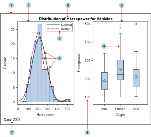
The following figure shows the different parts of a graph:

Figure 1.1 Components of a Graph

(10)

1 Graph

a visual representation of data. The graph can contain titles, footnotes, legends, and one or more cells that have one or more plots.

2 Cell

a distinct rectangular subregion of a graph that can contain plots, text, and legends.

3 Title

descriptive text that is displayed above any cell or plot areas in the graph.

4 Plot

a visual representation of data such as a scatter plot, a series line, a bar chart, or a histogram. Multiple plots can be overlaid in a cell to create a graph.

5 Legend

refers collectively to the legend border, one or more legend entries (where each entry has a symbol and a corresponding label) and an optional legend title.

6 Axis

refers collectively to the axis line, the major and minor tick marks, the major tick mark values, and the axis label. Each cell has a set of axes that are shared by all the plots in the cell. In multi‐cell graphs, the columns and rows of cells can share common axes if the cells have the same data type.

7 Footnote

descriptive text that is displayed below any cell or plot areas in the graph.

(11)

Chapter 2

Using the ODS GRAPHICS

Statement

About the ODS GRAPHICS Statement . . . 7

Using ODS Graphics Functionality to Create Graphs . . . 8

Using the ODS GRAPHICS Statement to Set Graphics Options . . . 10

Where to Go from Here . . . 10

About the ODS GRAPHICS Statement

The ODS GRAPHICS statement enables many SAS procedures to produce graphs as automatically as they produce tables. The statement enables or disables ODS graphics processing and sets graphics environment options.

Here is the basic syntax for the statement:

ODS GRAPHICS < OFF | ON> </ option(s)>;

The statement affects ODS graphical output only. (ODS graphs are template-based graphs that are created using Graph Template Language syntax. For more information, see “SAS/GRAPH Output versus ODS Graphics” on page 2.)

The statement can be used with any SAS procedure that supports ODS Graphics functionality. Like other ODS statements, the ODS GRAPHICS statement is global and can be used anywhere in your SAS program. The statement remains in effect until you explicitly change it or until you close the SAS session.

By default, the ODS GRAPHICS statement is set to ON for SAS procedures that support ODS Graphics when the procedures are executed in the SAS windowing environment on Windows and UNIX operating systems. In batch mode, the ODS GRAPHICS statement is set to OFF by default.

You can disable ODS Graphics output in the SAS preferences dialog box.

(12)

For more information, in SAS select Tools ð Options ð Preferences. Then click Help for the online documentation.

You can also disable ODS Graphics for the current SAS session by issuing the following statement.

ods graphics off;

T I P You should consider disabling ODS Graphics if your goal is solely to produce computational or tabular results. Producing ODS Graphics uses additional resources.

Using ODS Graphics Functionality to Create

Graphs

By default, ODS Graphics are enabled for many SAS procedures. However, you might need to request particular plots using procedure options. For procedures that support ODS Graphics, these options are described in the “Syntax” section of the procedure chapter of the respective user’s guide. You typically request graphs with the PLOTS= option in the procedure statement.

The following example uses the FREQ procedure to provide a frequency distribution based on the number of car cylinders. In this example, you do not need to specify the ODS GRAPHICS statement. ODS Graphics functionality is enabled by default for the FREQ procedure. However, this example specifies the PLOTS= option in the TABLES statement in order to produce graphical output.

title1 "Distribution of Cylinders"; proc freq data=sashelp.cars;

tables Cylinders / plots=freqplot; 8 Chapter 2 • Using the ODS GRAPHICS Statement

(13)

run; title1;

Note: The PLOTS= FREQPLOT option is described in the “Syntax” section of the

FREQ procedure in Base SAS Procedures Guide: Statistical Procedures.

Display 2.1 PROC FREQ Output Table

Display 2.2 PROC FREQ Output Graph

(14)

Using the ODS GRAPHICS Statement to Set

Graphics Options

You can use the ODS GRAPHICS statement options to control many aspects of your graphics. The settings that you specify remain in effect for all graphics until you change or reset these settings with another ODS GRAPHICS statement.

For example, if you are creating a graph for a paper or presentation, it is recommended that you specify the size of the graph as it will appear in the document rather than resize the graph after it has been produced. You can use options in the ODS GRAPHICS statement to control the size of the output image. The following example specifies a width of four inches and no border around the graph.

ods graphics / width=4in border=off; title1 "Cholesterol Levels for Age > 60"; proc sgpanel data=sashelp.heart(

where=(AgeAtStart > 60)) ; panelby sex / novarname;

loess x=weight y=cholesterol / clm; run;

title1;

Note: The height does not need to be specified in this example. The default aspect of the

graph is maintained when only the WIDTH= option is specified.

Display 2.3 Graph with a Width of Four Inches, and with No Border

Where to Go from Here

For more information about the ODS GRAPHICS statement, see “ODS GRAPHICS Statement” in SAS Output Delivery System: User's Guide.

(15)

Chapter 3

Using the ODS Graphics

Procedures

About the ODS Graphics Procedures . . . 11

Basic Structure of a Typical Procedure . . . 12

The SGPLOT Procedure . . . 12

The SGPANEL Procedure . . . 13

The SGSCATTER Procedure . . . 14

Examples of Using the Procedures . . . 14

SGPLOT Examples . . . 14

SGPANEL Example . . . 16

About the ODS Graphics Procedures

The ODS Graphics procedures produce plots for exploratory data analysis and for customized statistical displays. These procedures can produce a variety of single- and multi-cell plots and charts, including density, dot, needle, series, bar, histograms, box, and others. They can also compute and display loess fits, polynomial fits, penalized B-spline fits, reference lines, bands, and ellipses. Options are available for specifying colors, marker symbols, and other attributes of plot features.

These procedures use the Graph Template Language (GTL) to define the layout and details of a graph. Because SAS provides a default template for every graph produced by the procedures, you do not need to know anything about templates to create graphs with these procedures. You can create effective graphs with a minimal amount of learning and effort.

These are the ODS Graphics procedures: SGPLOT

creates single-cell plots with a variety of plot and chart types and overlays. SGPANEL

creates classification panels for one or more classification variables. Each graph cell in the panel can contain either a simple plot or multiple, overlaid plots. This procedure can create most of the plots that the SGPLOT procedure creates. For this reason, the two procedures have a similar syntax.

SGSCATTER

creates scatter plots and scatter plot matrices with optional fits and ellipses.

(16)

SGDESIGN

creates graphical output based on a graph file that has been created by using the ODS Graphics Designer application.

SGRENDER

produces graphs from graph templates that are written in the GTL. You can also render a graph from a SAS ODS Graphics Editor (SGE) file.

The procedures have two facilities that enable you to modify graph output:

• The SG annotation feature enables you to add shapes, images, and other annotations to graph output. This feature is preproduction in SAS 9.3.

• SG attribute maps enable you to control the visual attributes that are applied to specific data values in your graphs. For example, if an ODS Graphics procedure creates a graph that plots items sold in different countries, you can specify the display attributes for the sales data of each country. Attribute maps enable you to ensure that particular visual attributes are applied to data values in particular groups.

Basic Structure of a Typical Procedure

In general, an ODS Graphics procedure contains a procedure statement and one or more plot statements. The procedure statement typically specifies a data set. A procedure can have optional statements, such as axis statements and ODS statements. This section shows typical syntax for the SGPLOT, SGPANEL, and SGSCATTER procedures. (The SGDESIGN procedure is discussed in “Using SGD Files with the SGDESIGN

Procedure” on page 31. The SGRENDER procedure is shown in Chapter 4, “Using the Graph Template Language ,” on page 19.)

The SGPLOT Procedure

Here is a typical SGPLOT procedure. The procedure requires a procedure statement and at least one plot statement. Both statements accept options that provide more control over the appearance or behavior of the output. In this example, the GROUP= option is used to group the data and make it easier to interpret (when viewed in a color medium).

proc sgplot data=sashelp.class; /* procedure statement */

scatter x=height y=weight / group=sex; /* plot statement with a group option*/ run;

(17)

Display 3.1 Output for the SGPLOT Procedure

The SGPANEL Procedure

Here is a typical SGPANEL procedure, which creates a panel of graph cells for the values of one or more classification variables. The procedure requires a procedure statement, a classification statement (PANELBY), and at least one plot statement.

proc sgpanel data=sashelp.class; /* procedure statement */ panelby sex; /* classification statement */ scatter x=height y=weight; /* plot statement */

run;

Display 3.2 Output for the SGPANEL Procedure

(18)

The SGSCATTER Procedure

Here is a typical SGSCATTER procedure, which creates a paneled graph of scatter plots for multiple combinations of variables, depending on the layout statement that you use. The procedure requires a procedure statement and one of these three statements:

PLOT creates a paneled graph of scatter plots where each graph cell has its own independent set of axes.

COMPARE creates a shared axis panel, also called an MxN matrix. MATRIX creates a scatter plot matrix.

This example plots the values of two combinations of Y and X variables and produces a separate cell for each combination. That is, each Y*X pair is plotted on a separate set of axes.

proc sgscatter data=sashelp.cars; /* procedure statement */ plot mpg_highway*weight msrp*horsepower; /* plot statement */ run;

Display 3.3 Output for the SGSCATTER Procedure

Examples of Using the Procedures

SGPLOT Examples

Example Fit Plot

If you calculate a custom fit for your data, you might use a series plot to render the fit. The following PROC SGPLOT example combines a scatter and a series plot, and uses the SASHELP.CLASSFIT data set.

(19)

Display 3.4 Example Output for the FIT Plot

proc sgplot data=sashelp.classfit noautolegend; scatter x=height y=weight;

series x=height y=predict; run;

The NOAUTOLEGEND option in the SGPLOT statement disables the legend that is generated automatically for the graph. Without this statement, the graph would have an unnecessary legend, as seen below.

Display 3.5 FIT Plot with an Unnecessary Legend

Example Bar Chart

The following horizontal bar chart shows cumulative product orders for a clothing store.

(20)

Display 3.6 Bar Chart That Shows Cumulative Product Orders

In the SGPLOT procedure, the HBAR statement specifies the plot to be displayed, which in this case is a horizontal bar chart. In addition, the statement specifies the response variable (Number of Items) to be displayed on the horizontal axis. The response variable is optional. If you do not provide a response variable, then the chart shows the frequency count on the horizontal axis. The statement also specifies the statistic for the horizontal axis. The STAT= option enables you to specify the sum, the mean, or the frequency for the response variable.

proc sgplot data=sashelp.orsales; format Quantity comma7.;

hbar Product_Category / response = Quantity stat=sum; run;

Note also that the SGPLOT procedure supports the FORMAT statement, along with several other global SAS statements.

SGPANEL Example

The following example shows a panel of regression curves.

(21)

Display 3.7 Output for a Regression Plot

The COLUMNS= option in the PANELBY statement specifies that the panel has three columns of graph cells. The example uses the REG statement to create the regression curve. The CLI option creates individual predicted value confidence limits. The CLM option creates mean value confidence limits.

proc sgpanel data=sashelp.iris;

title "Scatter plot for Fisher iris data"; panelby species / columns=3;

reg x=sepallength y=sepalwidth / cli clm; run;

title;

Where to Go from Here

For more information and to learn about the syntax for the ODS Graphics procedures, see SAS ODS Graphics: Procedures Guide.

For information about individual procedures in that book, see the following chapters: • Chapter 4, “SGPANEL Procedure” in SAS ODS Graphics: Procedures Guide • Chapter 5, “SGPLOT Procedure” in SAS ODS Graphics: Procedures Guide • Chapter 7, “SGSCATTER Procedure” in SAS ODS Graphics: Procedures Guide

(22)

(23)

Chapter 4

Using the Graph Template

Language

About the Graph Template Language . . . 19

Basic Structure of a Typical Graph Template . . . 20

Example of Creating a Template . . . 21

About the Graph Template Language

For situations that require highly customized displays that are not available with the ODS Graphics procedures, you can write your own graph templates. You write templates using the Graph Template Language (GTL). A graph template is a program that specifies the layout and details of a graph. You can then apply the template to your data and render graphs using either the SGRENDER procedure or a DATA step. The GTL is a powerful language that includes statements for specifying the following graphics items:

• plot layouts, such as lattices and overlays • plot types, such as scatter plots and histograms • text elements, such as titles, footnotes, and insets

The GTL also provides support for built-in computations (such as histogram binning and loess smoothing) and the evaluation of expressions. The GTL supports dynamic variable assignment and conditional logic. Options are available for specifying colors, marker symbols, and other attributes of plot features.

In addition, the GTL has two features that enable you to customize a graph:

• Draw statements enable you to draw visual elements anywhere within the graph. For example, you can add text, lines, shapes, and images to a graph.

• Discrete and range attribute maps enable you to map visual attributes to input data values.

Procedure writers use the GTL to define graphs that procedures generate automatically in the process of an analysis. SAS analytical users can create very sophisticated graphs using terminology familiar to statisticians and analysts. However, with its robust capabilities and flexibility, the GTL requires an investment of time in order to learn how to best use it.

Here are two common uses for the GTL:

(24)

• create highly customized displays by writing your own graph templates and applying them directly to data with the SGRENDER procedure.

• modify the default SAS templates to make changes that are permanently in effect each time a particular procedure is executed. SAS provides a default template for every graph produced by statistical procedures.

The default graph templates provided by SAS are usually long and complex because they specify a complete description of how the graph is to be produced. You can edit graph templates to make simple modifications such as changing titles and axis labels or adding footnotes. Advanced users can make more substantive changes. This getting-started guide does not cover changes to the default graph templates.

Basic Structure of a Typical Graph Template

Graphs are constructed from two underlying components: a data object supplied by a procedure at run time and a compiled template that is designed to work with this data object. Together, the data object and the template form an output object that ODS displays in one or more output destinations.

All graph GTL programs use the TEMPLATE procedure to define a STATGRAPH template. Here is a short GTL program.

proc template; /* procedure statement */ define statgraph customGraphs.scatter; /* graph definition statement */ begingraph; /* container statement */ layout overlay; /* layout block statement */ scatterplot X=height Y=weight; /* plot statement */

endlayout; /* close the layout block */ endgraph; /* close the container block */ end; /* close the graph definition */ run;

Here are the noteworthy features of this program:

• The DEFINE STATGRAPH statement is required to open a definition block that defines and names the graph template. The END statement closes the template definition.

• A BEGINGRAPH statement block is required to define the outermost container for the graph. It must contain at least one LAYOUT block. The ENDGRAPH statement closes the container block.

• The LAYOUT statement block is required for specifying the layout structure of the graph. To generate a plot, the layout block must contain at least one plot statement. The ENDLAYOUT statement closes the layout block.

The TEMPLATE procedure must be run to compile the template and save it in the template store.

The template can be executed using the SGRENDER procedure. The procedure uses the DATA= option to specify the data source and the TEMPLATE= option to specify the template to use for rendering the graph.

Here is an example SGRENDER procedure:

proc sgrender data= sashelp.class template= customGraphs.scatter; run;

(25)

Note: In this example, the data set must contain the variables that are specified in the

plot statement of the template.

Display 4.1 Scatter Plot Output for the SGRENDER Procedure

Example of Creating a Template

This example creates a two-celled graph that shows linear and loess regression fits. The template uses a LATTICE layout with two columns.

Display 4.2 Two-Celled Linear and Loess Regression Graph

(26)

Here is the code for the output display.

proc template;

define statgraph mygraph; dynamic XVAR YVAR;

begingraph / designwidth=480px designheight=320px; layout lattice / columns=2;

layout overlayequated / equatetype=square; entry "Linear Regression Fit" /

valign=top textattrs=(weight=bold);

scatterplot x=XVAR y=YVAR / markerattrs=(color=red) datatransparency=.7; regressionplot x=XVAR y=YVAR;

endlayout;

layout overlayequated / equatetype=square; entry "Loess Fit" /

scatterplot x=XVAR y=YVAR / markerattrs=(color=red) datatransparency=.7; loessplot x=XVAR y=YVAR;

endlayout; endlayout; endgraph; end; run;

proc sgrender data=sashelp.iris template=mygraph; dynamic xvar="SepalLength" yvar="SepalWidth"; run;

Here is a brief description of the code.

• The DYNAMIC statement creates dynamic variables named XVAR and YVAR. This feature enables you to specify different names for the X and Y data values when you render the graph.

dynamic XVAR YVAR;

• The DESIGNWIDTH= and DESIGNHEIGHT= options in the BEGINGRAPH statement control the graph size.

begingraph / designwidth=480px designheight=320px;

• The LAYOUT statement begins the outer LAYOUT block and specifies a lattice with two columns.

layout lattice / columns=2;

• The outer LAYOUT block contains two nested LAYOUT blocks, one for each overlay cell in the lattice. Each cell contains a scatter plot and a fit plot. The main distinction between the two cells is the type of fit plot. The first cell contains a regression plot and the second cell contains a loess plot.

An ENTRY statement specifies the text for each cell title. The title for the first cell is "Linear Regression Fit." In the second LAYOUT block, the title is "Loess Fit." The MARKERATTRS= option in the SCATTERPLOT statement specifies a red color for the scatter plot markers. In addition, 70% transparency is assigned to the scatter plot to increase the visibility of the fit plot.

layout overlayequated / equatetype=square; entry "Linear Regression Fit" /

scatterplot x=XVAR y=YVAR / markerattrs=(color=red) datatransparency=.7; 22 Chapter 4 • Using the Graph Template Language

(27)

regressionplot x=XVAR y=YVAR; endlayout;

layout overlayequated / equatetype=square; entry "Loess Fit" /

scatterplot x=XVAR y=YVAR / markerattrs=(color=red) datatransparency=.7; loessplot x=XVAR y=YVAR;

endlayout;

• The SGRENDER procedure specifies the library and data set to use for the graph. The DYNAMIC statement specifies which columns to use for the X and Y variables of the graph, respectively.

proc sgrender data=sashelp.iris template=mygraph; dynamic xvar="SepalLength" yvar="SepalWidth"; run;

Where to Go from Here

For more information about the GTL and the SGRENDER procedure, see these documents:

• Chapter 2, “Quick Start,” in SAS Graph Template Language: User's Guide • SAS Graph Template Language: User's Guide

• SAS Graph Template Language: Reference

• Chapter 6, “SGRENDER Procedure” in SAS ODS Graphics: Procedures Guide

(28)

(29)

Chapter 5

Using the ODS Graphics Designer

About the ODS Graphics Designer . . . 25

About the Designer’s Graphical Interface . . . 25

Example of Using the Designer . . . 27

About This Example . . . 27

Step One: Create the First Cell and Assign Data . . . 27

Step Two: Add a Second Cell, Adjust Cell Height, and Use a Common Axis . . . . 30

Step Three: Customize the Title and Footnote . . . 31

Step Four: Save the Graph . . . 31 Using SGD Files with the SGDESIGN Procedure . . . 31

Using SGD Files with the Graph Template Language . . . 33

About the ODS Graphics Designer

The ODS Graphics Designer is an interactive graphical application that you can use to create and design custom graphs. The designer creates graphs that are based on the Graph Template Language (GTL). Using point-and-click interaction, you can create simple or complex graphical views of data for analysis without having to know the details of templates and the GTL.

The ODS Graphics Designer enables you to design sophisticated graphs by using a wide array of plot types. You can design multi-cell graphs, classification panels, and scatter plot matrices. Your graphs can have titles, footnotes, legends, and other graphics elements. You can save the results as an image for inclusion in a report or as an ODS Graphics Designer file (SGD) that you can later edit.

About the Designer’s Graphical Interface

The ODS Graphics Designer user interface consists of several main components, as shown in the following display:

(30)

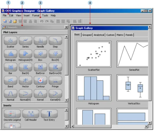
Figure 5.1 ODS Graphics Designer Graphical Interface

1 Main menu bar

contains menus that you can use to perform these tasks: • open, save, print, and edit SGD files

• open the Graph Gallery or view the code for a graph • insert titles, footnotes, and legends

• add rows and columns to the graph

• apply a different style to a graph, customize styles, and define new styles • set properties for graphs, plots, axes, legends, and other graph elements • set display and usage preferences for the designer

Note: In addition to the main menu, the designer has context menus that you can

open by right-clicking various parts of a graph.

2 Elements pane

contains plots, lines, and insets that you can insert into a graph. To insert an element, click and drag the element to the graph. The elements on this pane are available only when a graph is open.

3 Toolbar

contains icons that you can click to perform commonly used tasks such as saving files and inserting titles or footnotes. The icons on this toolbar are available only when a graph is open.

4 Work area

(31)

contains one or more graphs that you create and design in the designer. In addition to the graphs, you can display the Graph Gallery, a collection of predefined graphs.

Example of Using the Designer

About This Example

In this example, you create a paneled graph with two cells, each containing different types of plots. The graph shows the horsepower distribution for automobiles. The example uses the SASHELP.CARS data.

Display 5.1 Two-Cell Graph Example

There are several ways to create and customize this graph. The following steps show one way to create the graph.

Step One: Create the First Cell and Assign Data

1. Start the ODS Graphics Designer. In the SAS windowing environment, select Tools

ð ODS Graphics Designer. The designer opens and displays the Graph Gallery. 2. On the Basic tab of the Graph Gallery, double-click the Histogram icon.

(32)

The Assign Data dialog box appears. When you create a graph from the Graph Gallery, the graph has placeholder data assigned to its plot. The Assign Data dialog box enables you to easily change the data that is associated with the plot.

3. In the Assign Data dialog box, complete these steps: • Select SASHELP from the Library list box. • Select CARS from the Data Set list box. • Select HORSEPOWER from the X list box.

4. Click OK.

(33)

5. From the Plot Layers panel of the Elements pane, click and drag the Normal icon to the graph.

The Assign Data dialog box appears.

6. In the Assign Data dialog box, do not change the default selections.

Click OK. A normal curve is added to your graph. Here are the results of your graph so far.

(34)

Step Two: Add a Second Cell, Adjust Cell Height, and Use a Common Axis

1. Right-click anywhere within the plot area and select Add a Row. A new row cell is added below the histogram.

2. From the Plot Layers panel, click and drag the Box(H) icon to the new cell. The Assign Data dialog box appears.

3. In the Assign Data dialog box, complete these steps: • Select SASHELP from the Library list box. • Select CARS from the Data Set list box. • Select HORSEPOWER from the Y list box. 4. Click OK.

Both cells in the graph currently have the same height. In the next step, you adjust the cell height so that the histogram has more space.

5. To adjust the height of the two cells:

a. Position the cursor between the two cells of the graph. A dashed line appears between the cells and the cursor changes to a two-headed arrow .

b. Click and drag the dashed line downward. The cell with the histogram becomes taller, and the cell with the box plot becomes shorter.

6. Specify that both cells share a common X axis.

Right-click the bottom axis label and select Common Column Axis. Here are the results of your changes.

(35)

Step Three: Customize the Title and Footnote

1. Double-click the placeholder title. The placeholder text is highlighted:

2. In the text box, enter Distribution of Horsepower.

3. In the bottom left corner of the graph, double-click the placeholder footnote. The placeholder text is highlighted.

4. In the text box, enter Data: 2004.

Step Four: Save the Graph

Save this graph so that you can later return to it. The next section references this example.

1. Select File ð Save As.

2. Save the file to the desired location. Specify the name that you want for the file. For example, you might enter horsepower. The file type SGD Files (*.sgd) is selected by default.

3. Click Save.

Using SGD Files with the SGDESIGN Procedure

You do not need to know programming details to use the designer. However, with some knowledge of ODS Graphics procedure syntax, you can use the SGDESIGN procedure to produce graphical output from an SGD file. The procedure enables you to run one or

(36)

more graphs in batch mode and render the graphs to an ODS destination using any of the supported ODS options.

Here is the basic syntax for the procedure:

PROC SGDESIGN SGD= "SGD-file-specification" < option(s)>;

DYNAMIC dynamic-var–1="assigned-value–1" <dynamic-var–n="assigned-value-n">;

If the SGD file has been defined with shared variables, then you can substitute a different value for a variable by using the DYNAMIC statement. For more information about creating SGD files with shared variables, see Chapter 19, “Using Shared Variables in Graphs,” in SAS ODS Graphics Designer: User's Guide.

The following example uses the SGD file that was created in the previous example. (See

“Example of Using the Designer” on page 27.)

proc sgdesign sgd="C:\SGDFiles\horsepower.sgd"; run;

Note the following about the procedure:

• In the SGD= option of the procedure statement, substitute the path to your SGD file. • The example does not need to specify the SASHELP.CARS data set. By default, the

SGDESIGN procedure uses the data set that is defined in the SGD file.

Display 5.2 PROC SGDESIGN Output for the Horsepower Distribution Graph

Note: Graphs that are output to the default ODS destination in SAS might look different

from those that were created using the designer's default style. In the SAS

windowing environment, HTML is the default ODS destination, and HTMLBlue is the default style. The default style for the ODS Graphics Designer is Listing (although you can change that in the Preferences). See “Changing the Style That Is Applied to ODS Graphs” on page 45 for details about specifying a style for a graph either in the SAS program or in the designer.

(37)

For another example that uses the SGDESIGN procedure, see “Example of Producing an Annotated ODS Graphics Designer Graph for Publication” on page 55.

Using SGD Files with the Graph Template

Language

You do not need to know about the Graph Template Language (GTL) in order to use the designer. However, if you do know details of the GTL, you can use the code that is generated for an SGD file to design custom templates.

Here are the main steps:

1. In ODS Graphics Designer, select the graph to make it active. Then select View ð

Code. A window appears and displays the code for the graph.

2. To copy the code, select the portion of the code that you want, and then select Edit

ð Copy.

T I P To select the entire code, select Edit ð Select All.

You can now paste the code into SAS and customize the graph template using the GTL.

3. To save the code as a SAS program, select File ð Save As. Then specify the location and filename for the code.

4. Select View ð Code again to close the code window, or click the Close button in the window.

Where to Go from Here

To get started with the ODS Graphics Designer, see Chapter 3, “Quick-Start Examples,” in SAS ODS Graphics Designer: User's Guide.

For complete information about using the ODS Graphics Designer, see SAS ODS

Graphics Designer: User's Guide.

For more information about the SGDESIGN procedure, see Chapter 3, “SGDESIGN Procedure” in SAS ODS Graphics: Procedures Guide.

(38)

(39)

Chapter 6

Using the ODS Graphics Editor

About the ODS Graphics Editor . . . 35

About the Editor’s Graphical Interface . . . 36

Example of Using the Editor . . . 37

About This Example . . . 37

Step One: Create and Open an Editable Graph . . . 38

Step Two: Add and Format a Title . . . 38

Step Three: Modify the Axis Labels . . . 39

Step Four: Add and Rotate a Text Annotation . . . 39

Step Five: Change the Style and Print the Graph . . . 40

Step Six: Save the Graph . . . 40 Where to Go from Here . . . 40

About the ODS Graphics Editor

If you want to make immediate changes to a particular graph, such as change the title or add a text inset or an image, you can use the ODS Graphics Editor. The editor is an interactive graphical application used to edit and annotate graphs that are created by any SAS procedure that supports ODS Graphics. The graphic must be an ODS Graphics Editor file (SGE), which is created in SAS by using the SGE = ON option in the ODS destination statement.

You can customize titles, footnotes, and labels. You can annotate data points, add text, and change graph element properties such as fonts, colors, markers, and line styles. After you have modified your graph, you can save it in one of several formats or as an SGE file that you can later reopen and edit.

You can also use the SGRENDER procedure (in the ODS Graphics procedures) to produce graphical output from the SGE file. The procedure enables you to run one or more graphs in batch mode and render the graphs to any ODS destination using any of the supported ODS options.

You can launch the editor from a SAS session. You can also download a stand-alone version of the ODS Graphics Editor that runs independently of SAS. When you edit a graph from the Results window in SAS, changes that you make do not affect the original graph in the Results Viewer window.

(40)

About the Editor’s Graphical Interface

The ODS Graphics Editor user interface consists of several main components, as shown in the following display:

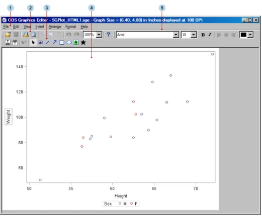
Figure 6.1 ODS Graphics Editor Graphical Interface

1 Main menu bar

contains menus that you can use to perform these tasks: • open, save, and print SGE files

• copy and paste items, and change the view (zoom and toolbars) • insert titles, footnotes, and annotations

• arrange, group, and order annotations • move titles and footnotes up or down

• apply a different style to a graph, and set graph properties

Note: In addition to the main menu, the editor has context menus that you can access

by right-clicking various parts of a graph.

2 Standard toolbar

provides access to file operations, such as print, copy, paste, and undo.

3 Graph toolbar

(41)

provides an easy way to select graph objects or to insert items into a graph. For more information, see “About the Graph Toolbar” in Chapter 2 of SAS ODS Graphics

Editor: User's Guide. 4 Work area

contains the graph that you want to edit or annotate.

5 Formatting toolbar

provides formatting tools that enable you to change the font, size, color, and other attributes of text elements and annotations.

Note: This toolbar is active only if you have text or annotation objects selected in

your graph. The text element that you select might be a title, footnote, an axis label, or a legend.

Example of Using the Editor

About This Example

This example shows how you might edit and annotate a graph that was created with the SGPLOT procedure. These tasks use some of the toolbar functions previously described. At the completion of the tasks in this example, the resulting graph is displayed:

Display 6.1 Edited and Annotated Graph Example

(42)

Step One: Create and Open an Editable Graph

1. In SAS, execute the following code. The SGE = ON option in the ODS destination statement creates an editable graph.

ods html sge = on; /* enable editable graph creation */ proc sgplot data=sashelp.class; /* procedure statement */

scatter x=height y=weight /* plot statement with a group option*/ / group=sex;

run;

ods html sge = off; /* disable editable graph creation */

The SAS Results Viewer displays a scatter plot, shown here.

Your program also created an ODS Graphics Editor (SGE) file that you can edit. 2. Locate this SGE file by selecting View ð Results from the main menu.

3. Click the expansion icon in the SAS Results window to show the SGE file just created with the SGPLOT procedure.

4. Double-click the SGE file, which is identified by the icon.

The ODS Graphics Editor opens and displays the graph for editing. You are now ready to edit the graph using the various interactive tools built into the editor.

a. In the Formatting toolbar at the top of the window, select the Arial Rounded

MT Bold font from the font drop-down list

Note: If the Formatting toolbar is dimmed, select the title to make the toolbar

available.

b. Click the Bold button to undo the text boldface, and the Italic button to italicize the text.

c. Press ENTER to preserve your formatting selections.

Step Three: Modify the Axis Labels

1. Double-click the Height X-axis label.

2. Move your cursor to the end of the text and type (IN). 3. Press ENTER to preserve the new text.

4. Double-click the Weight Y-axis label.

5. Move your cursor to the end of the text and type (LBS). 6. Press ENTER to preserve the new text.

Step Four: Add and Rotate a Text Annotation

1. Click the Text button in the Graph toolbar.

2. Click the area of the graph where you want to position your text—for example the lower right quadrant of the graph. A text box appears.

3. Enter My annotation text in the box. The width of the text box determines the maximum width of the text line. If a line exceeds the width of the text box, then the text wraps to the next line. If needed, drag one of the circles on the border of the text box to the right or left to widen the text box.

4. To rotate the text annotation, follow these steps: a. Position your cursor in the circle above the text box.

The cursor changes to a rotated arrow.

b. Click and drag the rotated arrow to the left or right. You can rotate the entire box anywhere within a 360 degree radius.

5. Click anywhere in the graph outside the text box to preserve the text.

(44)

Step Five: Change the Style and Print the Graph

By default, graph SGE files use the active ODS destination style that is specified in the SAS program. If no style is specified, then the default style is used for the ODS destination.

1. Change the graph’s style in order to make the graph more suitable for printing with a black-and-white printer.

Select Format ð Style ð Journal from the main menu.

Note: When you apply the Journal style, all of the graphics elements change to

shades of gray. However, if you had specified a different color for an element, the color would not change. When you explicitly set a color or other attribute, the specified attribute overrides the style setting.

2. Print your edited and annotated SGE file. a. Select File ð Print from the main menu bar. b. Select print options from the Print window. c. Click OK.

Note: You can also print PNG files from the ODS Graphics Editor. Or you can

include a PNG file in a PDF document and then print the PDF document.

Where to Go from Here

This chapter has given you a general overview of the ODS Graphics Editor, and walked you through an example of creating and editing a SAS SGE file. You can obtain more information in the following places:

• For an example that shows how to edit and annotate a graph that was created in the ODS Graphics Designer, see “Example of Producing an Annotated ODS Graphics Designer Graph for Publication” on page 55.

• For more examples and to learn all the details about using the ODS Graphics Editor, see SAS ODS Graphics Editor: User's Guide.

(45)

• For more information about editable graphs in particular, see “Creating Editable Graphics ” in Chapter 2 of SAS ODS Graphics Editor: User's Guide.

• For more information about annotating graphs, see Chapter 8, “Annotation Overview,” in SAS ODS Graphics Editor: User's Guide.

• For more information about the ODS Graphics procedures, see SAS ODS Graphics:

Procedures Guide.

(46)

(47)

Chapter 7

Changing the Appearance of

Graphs

Understanding ODS Styles . . . 43

About Styles and Style Elements . . . 43

About the Default Styles . . . 44 Recommended Styles for Statistical Work . . . 44

Working with Styles . . . 45

Changing the Style That Is Applied to ODS Graphs . . . 45

Editing a Style . . . 47

Changing the Appearance of Individual Graphics Elements in a Plot . . . 48 Using Attribute Mapping . . . 51

Adding Annotations to Graphs . . . 51

Understanding ODS Styles

About Styles and Style Elements

ODS styles are produced from compiled STYLE templates written in PROC

TEMPLATE style syntax. An ODS style template is a collection of style elements that provides specific visual attributes for your SAS output.

Each style element is a named collection of style attributes such as color, marker symbol, line style, font face, as well as many others. For example, a density plot uses the GraphFit style element for its visual attributes. The GraphFit style element has attributes for color, line style, line thickness, and so on.

Each graphical element of a plot, such as a marker, a line, or a title, derives its visual properties from a specific style element from the active style. The style elements of a style are designed to ensure the goals of effective graphics.

The easiest way to change a graph's appearance is to change the style that the graph uses. For more information, see “Changing the Style That Is Applied to ODS Graphs” on page 45.

Recommended Styles for Statistical Work

SAS styles have been designed to address the needs of different situations while ensuring the principles of effective graphics. The following is a subset of the styles shipped with SAS that are particularly suited for statistical graphics:

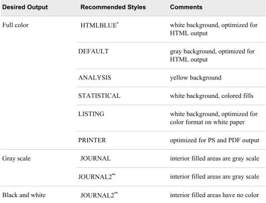
Table 7.1 Recommended Styles

Desired Output Recommended Styles Comments

Full color HTMLBLUE* _{white background, optimized for}

HTML output

DEFAULT gray background, optimized for HTML output

ANALYSIS yellow background

STATISTICAL white background, colored fills LISTING white background, optimized for

color format on white paper PRINTER optimized for PS and PDF output Gray scale JOURNAL interior filled areas are gray scale JOURNAL2** _{interior filled areas are gray scale}

Black and white JOURNAL2** _{interior filled areas have no color}

* HTMLBlue is the default style for the ODS HTML destination.

** When used with the ODS Graphics procedures, Journal2 and Journal3 by default render grouped bars with fill patterns.

(49)

Working with Styles

Changing the Style That Is Applied to ODS Graphs Changing the Style in Your Program

When you use the ODS Graphics procedures or the Graph Template Language, you can easily change a graph's appearance by changing the style for an ODS destination. Changing the current style requires only the use of the STYLE= option in an ODS destination statement. The ODS destination statement is global and can be used anywhere in your SAS program. The statement remains in effect until you explicitly change it or start a new SAS session.

Note: The style that a destination uses is applied to tabular output as well as graphical

output.

In the following example, the ODS destination statement specifies HTML as the destination and HTMLBlue as the style.

ods html style=htmlblue; title "Model Height By Weight"; proc sgplot data=sashelp.class; reg x=height y=weight / clm cli; run;

title;

Display 7.1 HTML Output Using the HTMLBlue Style

The following displays show the output for the same graph when the STYLE= option is specified as Analysis and Journal, respectively.

(50)

Display 7.2 HTML Output Using the Analysis Style

Display 7.3 HTML Output Using the Journal Style

Changing the Style in the ODS Graphics Designer or the ODS Graphics Editor

In the ODS Graphics Designer and the ODS Graphics Editor, you can use the menus to change the style for a particular graph.

• In the ODS Graphics Designer, one way to change the style for a graph is to right-click the graph and select Graph Properties. In the Graph Properties dialog box, clicking the down arrow in the Style drop-down list displays the styles that are available.

(51)

Display 7.4 Styles in the Graph Properties Dialog Box (ODS Graphics Designer)

The default style for graphs created in the designer is Listing. You can change this default in the designer’s preferences.

• The ODS Graphics Editor has a similar interface for changing the style of a graph. In the editor, you can change the style for a graph by selecting Format ð Style. Then select the style that you want.

By default, ODS Graphics Editor files use the active ODS destination style that is specified in the SAS program.

Editing a Style

ODS styles are based on templates that define the specific visual attributes for your SAS output. You can use the following software to edit style templates:

• TEMPLATE procedure

You can modify the ODS style template for a style to make persistent changes to that style. Using the TEMPLATE procedure, you can modify the default SAS style templates as well as custom styles that have been created at your site.

For more information about the TEMPLATE procedure, see SAS Output Delivery

System: User's Guide.

• ODS Graphics Designer

The ODS Graphics Designer has an interactive graphical interface for designing and modifying custom styles. This interface, called the Graph Style Editor, makes it easy to design styles that you can apply to your SGD graphs. You can also use these custom styles for graphs that are generated outside of the designer.

Here is a high-level overview of the process using the ODS Graphics Designer

(52)

1. In the designer, open the Graph Style Editor. Select Tools ð Style Editor.

2. Create or modify a custom style. You cannot change the predefined SAS ODS styles. However, you can edit a SAS style, customize various style elements and attributes, and save your changes using a new style name.

For complete instructions about creating custom styles, see Chapter 13, “Customizing Graph Styles,” in SAS ODS Graphics Designer: User's Guide. 3. Apply the custom style to your ODS Graphics Designer graphs as appropriate. 4. You can also use the style when you generate graphs outside of the ODS Graphics

Designer. Follow these steps:

a. To export the style, select File ð Export Style and select the style (or styles) that you want to export.

b. Run the exported code in SAS to compile a style and save it in the style template store.

c. Do either or both of the following:

• Apply the style to your procedures by specifying the style in the ODS destination statement.

• Modify the style using the TEMPLATE procedure.

Changing the Appearance of Individual Graphics Elements in a Plot Overview of Changing Graphics Elements

ODS Graphics software enables you to control the appearance of different parts of a graph without changing the overall style. For example, you can change the visual attributes of lines, bars, markers, text, and so on. These changes are limited to the current graph.

Each graphics element of a plot, such as a marker or a line, derives its visual attributes from a specific style element from the active style. Within a given style, the style elements give you more granular control of a graph's visual elements.

In general, there are two ways to change the appearance of a graphics element: • You can specify a different style element for the graphics element. For example, a

density curve uses the default GraphFit style element for its visual attributes. You might instead specify the GraphFit2 style element.

• You can change one or more attributes of a style element. For example, you might explicitly change the color of a density curve to red.

It is recommended that you specify style elements rather than explicit attributes whenever possible. The attributes of a style element are chosen to provide consistency and appropriate emphasis based on display principles for statistical graphics. When you specify a particular attribute, you override the style element. You might create a graph that is inconsistent with the style. If you later change the style for the graph, your override remains in effect and could clash with the new style.

Note: For bar charts, you also have the option to specify one of several bar skins. This

option provides an easy way to enhance the appearance of the bars. The option is supported in the Graph Template Language, in the ODS Graphics procedures, and in the ODS Graphics Designer.

(53)

The following sections describe the options for changing the appearance of graphics elements in the ODS Graphics software.

Changing Graphics Elements in Your Program

The ODS Graphics software gives you the following options for changing the appearance of graphics elements in your program:

• ODS Graphics procedures

Many ODS Graphics procedure statements have options and suboptions that control the appearance of different parts of a graph. Typically, you can specify a style element, a hardcoded attribute value, or a combination of both. The following example specifies a style element for a density curve in a graph.

proc sgplot data=sashelp.class noautolegend; density height / lineattrs=graphfit2; run;

The following displays show the default and the modified appearance.

Default Line Attributes GRAPHFIT2 Line Attributes

The following example specifies a style element and a hardcoded attribute value. This example changes the line to a dash-dash-dot pattern ( ).

density height / lineattrs=graphfit2 (pattern=dashdashdot);

• Graph Template Language

The Graph Template Language uses similar syntax to specify a style element, a hardcoded attribute value, or a combination of both. The following example specifies the marker color for a scatter plot.

scatterplot x=XVAR y=YVAR / markerattrs=(color=red);

This example was taken from “Example of Creating a Template” on page 21.

Changing Graphics Elements in ODS Graphics Designer

The ODS Graphics Designer gives you numerous options for changing the appearance of graphics elements in an SGD file. You can use the designer’s graphical interface to specify the style element or the element attributes (color, font size, and so on) of a graphics element.

For example, to change the properties of a graph title, right-click the title and select Title

Properties from the pop-up menu. The following display shows the properties for a

graph title.

(54)

Display 7.5 GraphTitleText Style Element in the Text Properties Dialog Box

Changing Graphics Elements in ODS Graphics Editor

The editor enables you to change the visual attributes of a graphics element, but not the style element. For example, to change the properties of a graph title, right-click the title and select Compose Rich Text from the pop-up menu. From the Compose Rich Text dialog box, you can change the text and the font properties. You can also use subscript or superscript values, and you can enter Unicode characters.

Display 7.6 Compose Rich Text Dialog Box

(55)

Using Attribute Mapping

The attribute map feature enables you to control the visual attributes that are applied to specific data values in your graphs. For example, if a procedure creates a graph that plots items sold in different countries, you can specify the display attributes for the sales data of each country.

You can use the ODS Graphics procedures or the Graph Template Language to map visual attributes to input data values.

SAS 9.3 ODS Graphics. Getting Started with Business and Statistical Graphics. SAS Documentation

9.3 ODS Graphics

Contents

Chapter 1 • Introduction to ODS Graphics . . . 1

Chapter 3 • Using the ODS Graphics Procedures . . . 11

Chapter 5 • Using the ODS Graphics Designer . . . 25

Chapter 6 • Using the ODS Graphics Editor . . . 35

Chapter 8 • Understanding ODS Graphics Software Interactions . . . 53

Chapter 1

What is ODS Graphics? . . . 1

What is ODS Graphics?

See Also

SAS/GRAPH Output versus ODS Graphics

The Suite of ODS Graphics Software

See Also

Benefits of Using ODS Graphics Software

Overview of ODS Destinations

ODS destination <option(s);>

See Also

Components of a Graph

Figure 1.1 Components of a Graph

Chapter 2

About the ODS GRAPHICS Statement . . . 7

About the ODS GRAPHICS Statement

ODS GRAPHICS < OFF | ON> </ option(s)>;

Using ODS Graphics Functionality to Create

Display 2.1 PROC FREQ Output Table

Using the ODS GRAPHICS Statement to Set

Display 2.3 Graph with a Width of Four Inches, and with No Border

Where to Go from Here

About the ODS Graphics Procedures . . . 11

About the ODS Graphics Procedures

SGSCATTER

Basic Structure of a Typical Procedure

The SGPLOT Procedure

The SGPANEL Procedure

The SGSCATTER Procedure

Display 3.3 Output for the SGSCATTER Procedure

Examples of Using the Procedures

Example Fit Plot

Display 3.5 FIT Plot with an Unnecessary Legend

SGPANEL Example

Where to Go from Here

Language

About the Graph Template Language . . . 19

About the Graph Template Language

Basic Structure of a Typical Graph Template

Display 4.1 Scatter Plot Output for the SGRENDER Procedure

Example of Creating a Template

Display 4.2 Two-Celled Linear and Loess Regression Graph

Where to Go from Here

Chapter 5

About the ODS Graphics Designer . . . 25

Using SGD Files with the Graph Template Language . . . 33

About the ODS Graphics Designer

Figure 5.1 ODS Graphics Designer Graphical Interface

Example of Using the Designer

Display 5.1 Two-Cell Graph Example

4. Click OK.

Step Two: Add a Second Cell, Adjust Cell Height, and Use a Common Axis

Step Three: Customize the Title and Footnote

1. Select File ð Save As.

Using SGD Files with the SGDESIGN Procedure

PROC SGDESIGN SGD= "SGD-file-specification" < option(s)>;

Display 5.2 PROC SGDESIGN Output for the Horsepower Distribution Graph

Using SGD Files with the Graph Template

Code. A window appears and displays the code for the graph.

Where to Go from Here

Chapter 6

About the ODS Graphics Editor . . . 35

About the ODS Graphics Editor

See Also

About the Editor’s Graphical Interface

Figure 6.1 ODS Graphics Editor Graphical Interface

See Also

Example of Using the Editor

Display 6.1 Edited and Annotated Graph Example

See Also

a. In the Formatting toolbar at the top of the window, select the Arial Rounded

Step Three: Modify the Axis Labels