Development of Probability Based Intensity- Duration-Frequency Curves under Climate Change

THE UNIVERSITY OF WESTERN ONTARIO

DEPARTMENT OF CIVIL AND

ENVIRONMENTAL ENGINEERING

Water Resources Research Report

Report No: 072

Date: March 2011

Development of Probability Based

Intensity-Duration-Frequency Curves under Climate

Change

By:

Tarana A. Solaiman

and

Slobodan P. Simonovic

ISSN: (print) 1913-3200; (online) 1913-3219;

1

Development of Probability Based Intensity-Duration-Frequency

Curves under Climate Change

By:

Tarana A. Solaiman And

Slobodan P. Simonovic

Department of Civil and Environmental Engineering The University of Western Ontario

London, Ontario, Canada

2

Executive Summary

Hydrologic design of storm sewers, culverts, retention/detention basins and other components of storm water management systems are typically performed based on specified design storms derived from the rainfall intensity-duration-frequency (IDF) estimates and an assumed temporal distribution of rainfall. Use of inappropriate data or design storms could lead to malfunctions of the infrastructure systems: over-estimation may result in costly over-design or under-estimation may be associated with risk and human safety. One of the expected hydro-climatic impacts of climate change for London is the increase in the magnitude and frequency of extreme rainfalls which can have serious impact on the design, operation and maintenance of existing municipal water infrastructure.

This study presents a methodology for updating the rainfall IDF curves for the City of London incorporating various uncertainties associated with the assessment of climate change impacts on a local scale. Overall, two objectives have been achieved: first, an extensive investigation of the possible realizations of future climate from 29 scenarios developed from Atmosphere-Ocean Global Climate Models (AOGCM) and scenarios are performed using a downscaling based disaggregation approach. Annual maximum series of rainfall are fitted to Gumbel distribution to develop IDF curves for 1, 2, 6, 12 and 24 hour durations for 2, 5, 10, 25, 50 and 100 years of return periods. Next, the associated uncertainties are estimated using non-parametric kernel estimation approach and the resultant IDF curve is developed based on a probabilistic approach.

The results indicate that rainfall patterns in the City of London will most certainly change in future due to climate change. The use of the multi-model approach, rather than a single scenario

3

is encouraged. Inherent uncertainties associated with different AOGCMs are quantified by a kernel based plug-in estimation approach. The resultant scenario indicates approximately 20-40% changes in different duration rainfalls for all return periods. Use of a probability based intensity-duration-frequency curve is encouraged in order to apply the updated IDF information with higher level of confidence.

4

Table of Contents

1.2 Uncertainties in Atmosphere-Ocean Global Climate Models ... 10

1.3 Intensity-Duration-Frequency Curves ... 11

1.4 Outline of the Report ... 12

2. Literature Review... 14

3. Methodology ... 18

3.1 Database ... 18

3.1.1 Observations ... 18

3.1.2 Climate Change Scenarios ... 20

3.2 Development of Methodology ... 22

3.2.1 Downscaling ... 22

3.2.2 Bias Correction of Downscaled Outputs ... 26

3.2.3 Disaggregation ... 27

3.2.4 Generation of Rainfall for Different Durations ... 29

3.2.5 Intensity-Duration-Frequency Analysis ... 30

3.2.6 Uncertainty Quantification ... 32

5

4.1 Selection of Appropriate Stations ... 37

4.2 Development of Climate Change Scenarios... 40

4.3 Verification of the IDF Generation Methods ... 41

4.4 IDF Results for Future Climate ... 45

4.5 Uncertainty Quantification of IDF Results ... 49

5. Conclusions ... 55

Acknowledgments... 57

References ... 58

APPENDIX A: Regression Test Results ... 66

APPENDIX B: SRES Emission Scenarios ... 70

APPENDIX C: Atmosphere-Ocean General Circulation Models ... 72

APPENDIX D: Comparison of Future IDF Results in terms of Intensities (mm/hr) ... 81

APEPNDIX E: IDF Plots of Selected Scenarios ... 87

6

List of Tables

Table 1: Rain Gauge Station Details ... 19

Table 2: List of AOGCM Models and Emission Scenarios ... 21

Table 3: Groups for Regression Analysis based on Distances ... 38

Table 4: Cross-Correlation Results for Stations Within 200 km Distance from London ... 40

Table 5 (a): Monthly Mean Precipitation (mm) from Different AOGCMs for 1965-1990 ... 41

Table 6 (a): Comparison of Extreme Rainfall in London in terms of Depth (mm) ... 44

Table 6 (b): Relative Difference between EC IDF Information and Historic Unperturbed Scenario... 45

Table 7: Percent Differences between Historic Perturbed, Wet and Dry Scenarios ... 46

7

List of Figures

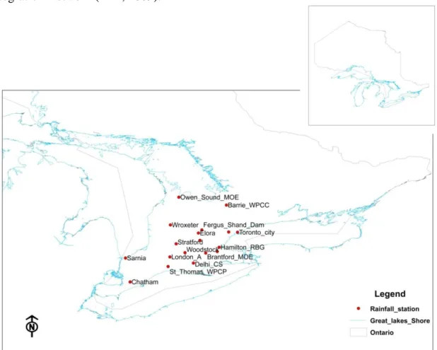
Figure 1: Meteorological Stations Used in the Study ... 18

Figure 2: Schematic Diagram of Developing IDF Curve ... 23

Figure 3: Performances of Stations based on Distance ... 39

Figure 4: Box and Whiskers Plot of Simulated Monthly Rainfall in London ... 42

Figure 5: Frequency Plots of Observed (Obs) and Simulated (Sim) Hourly Rainfall ... 43

Figure 6: IDF Plots of AOGCM Scenarios for Different Durations ... 48

Figure 7: Comparison of IDF Plots for Different Scenarios ... 51

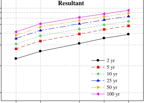
Figure 8: IDF Plot for Resultant Scenario ... 52

Figure 9 (a): Probability based IDF Curve of 1 and 2 Hour Duration ... 53

8

1. Introduction

1.1 Problem Definition

The increase of carbon dioxide concentration in the atmosphere due to industrial activities in the past and recent times has been identified as the major cause of global warming and climate change. The normal balance of Earth’s hydrological cycle has been altered due to the changes in the temperature and precipitation patterns. Projections from climate models suggest that the probability of occurrence of intense rainfall in future will increase due to the increase in green house gas emission (Mailhot and Duchesne, 2010). Research related to the analysis of extreme precipitation indices have projected an increase in the annual total precipitation during the second half of the past century; the number of days with precipitation is also expected to increase, with no consistent pattern for extreme wet events (Vincent and Mekis, 2005). Stone et al. (2000) reported seasonally increasing trends in total precipitation during the 20th century for southern parts of Canada resulting from increased heavy and intermediate events. Research related to the Upper Thames River basin (Solaiman and Simonovic, 2011) have also indicated that there is now higher probability that the occurrence of extreme precipitation events will be more frequent in future. Such changes in extreme events have enormous ecological, societal and economic impacts in the form of floods, droughts, heat waves, summer and ice storms and have great implications for municipalities: a small shift in the climate normals can have large consequences on the existing infrastructure; climate change will affect any municipalities (big or small, rural or urban) by damaging existing municipal infrastructure (bridges/roads), natural systems (watersheds, wetlands and forests) and human system (health and education) (Mehdi et al, 2006). The design standards at present are based on the historic climate information and required level of protection from natural phenomena. Under a changing climate, it has become a

9

priority for the municipalities to search for appropriate procedures, planning and management to deal with and adopt to changing climatic conditions. Decision makers and stakeholders need to understand the possible effects for developing suitable management decisions for the future. Possible changes may demand new regulations, guidelines for storm water management studies, revision and update of design practices and standards, or retrofitting of existing infrastructure or even constructing additional ones (Prodanovic and Simonovic, 2007).

Global scale climate variables are commonly projected by Coupled Atmosphere-Ocean Global Climate Models (AOGCMs) to provide a numerical representation of the climate system based on the physical, chemical and biological properties of their components and feedback interactions between them (IPCC, 2007). They are, currently the most reliable tools available for obtaining the physics and chemistry of the atmosphere and oceans and to derive projections of meteorological variables (temperature, precipitation, wind speed, solar radiation, humidity, pressure, etc). They are based on various assumptions about the effects of the concentration of greenhouse gases in the atmosphere coupled with projections of CO2 emission rates (Smith et al., 2009).

There is a high level of confidence that AOGCMs are able to capture large scale circulation patterns and correctly model smoothly varying fields such as surface pressure, especially at continental or larger scales. However, it is extremely unlikely that these models properly reproduce highly variable fields, precipitation (Hughes and Guttorp, 1994), on a regional scale, let alone, for small to medium watersheds. Although confidence has increased in the ability of AOGCMs to simulate extreme events, such as hot and cold spells, the frequency and the amount of precipitation during intense events are still being underestimated.

10

Present study aims to provide an insight into the future changes in the intensity of extreme rainfall events associated with model and scenario uncertainties and suggest methods for quantifying these uncertainties. The result is presented in the form of probability based intensity-duration-frequency (IDF) curves appropriate for the future climatic conditions.

1.2 Uncertainties in Atmosphere-Ocean Global Climate Models

In recent years, quantifying uncertainties from AOGCMs and scenarios for impact assessment studies has been identified as a critical climate change and adaptation research topic. Climate change impact studies derived from AOGCM outputs are associated with uncertainties due to “incomplete” knowledge originating from insufficient information or understanding of biophysical processes or a lack of analytical resources. Examples include simplification of complex processes involved in atmospheric and oceanographic transfers, inaccurate assumptions about climatic processes, limited spatial and temporal resolution resulting in a disagreement between AOGCMs over regional climate change, etc. Uncertainties also emerge due to “unknowable” knowledge arising from the inherent complexity of the Earth system and from our inability to forecast future socio-economic and human behavior in a deterministic manner (New and Hulme, 2000; Allan and Ingram, 2002; Proudhomme et al., 2003; Wilby and Harris, 2006; Stainforth et al., 2007; IPCC, 2007, Buytaert et al, 2009). It is now established that the accuracy of AOGCMs decrease at finer spatial and temporal scales; a typical resolution of AOGCMs ranges from 250 km to 600 km, but the need for impact studies conversely increase at finer scales. The representation of regional precipitation is distorted due to the coarse resolution and cannot capture the subgrid-scale processes significant for the formation of site-specific precipitation conditions. While some models are parameterized, details of the land-water distribution or topography in others are not represented at all (Widmann et al., 2003). Studies

11

have found that the models failed to predict the high variability in daily precipitation and could not accurately simulate present-day monthly precipitation amounts (Trigo and Palutikof, 2001; Brissette et al., 2006).

1.3 Intensity-Duration-Frequency Curves

Reliable rainfall intensity estimates are necessary for hydrologic analyses, planning and design problems. The rainfall intensity-duration-frequency (IDF) curve is one of the most common tools for urban drainage designer. Information from IDF curves are used to describe the frequency of extreme rainfall events of various intensity and durations. According to the guideline for ‘Development, Interpretation and Use of Rainfall Intensity-Duration-Frequency (IDF) Information: A Guideline for Canadian Water Resources Practitioners” developed by Canadian Standards Association (CSA, 2010), the major reasons for increased demand for rainfall IDF information can be summarized as follows:

 As the spatial heterogeneity of extreme rainfall patterns becomes better understood and documented, a stronger case is made for the value of “locally relevant” IDF information.

 As urban areas expand, making watersheds generally less permeable to rainfall and runoff, many older water systems fall increasingly into deficit, failing to deliver the services for which they were designed. Understanding the full magnitude of this deficit requires information on the maximum inputs (extreme rainfall events) with which drainage works must contend.

 Climate change will likely result in an increase in the intensity and frequency of extreme precipitation events in most regions in the future. As a result, IDF values will optimally need to be updated more frequently than in the past and climate change scenarios might eventually be drawn upon in order to inform IDF calculations.

12

The typical establishment of rainfall IDF curves involves three steps. First a probability distribution function (PDF) or Cumulative Distribution Function (CDF) is fitted to each group comprised of the data value for any specific duration. The maximum rainfall intensity for each time interval is related with the corresponding return period from the cumulative distribution function. For a given return period , the cumulative frequency can be expressed as:

If the cumulative frequency is known, the maximum rainfall intensity can be determined using an appropriate theoretical distribution function (such as Generalized Extreme Value (GEV), Gumbel, Pearson Type III, etc).

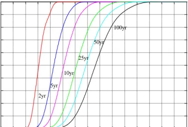
In the presence of climate change, the theoretical distribution based on historical observations will be different for the future conditions. The issue is further aggravated by the presence of various uncertainties associated with AOGCM models and emission scenarios. Therefore, in this study the non-parametric kernel estimator is used to combine uncertainties generated from different AOGCMs. Probability of occurrences of maximum rainfall generated for any specific duration is presented in the form of cumulative distribution function for different return periods.

1.4 Outline of the Report

The report is organized as follows: research related to IDF information under climate is presented in Chapter 2. Chapter 3 details the database and methodology applied in the study. The

13

results and discussion obtained from the analysis are explained in Chapter 4. Finally the report ends with conclusions based on the research findings.

14

2. Literature Review

Literature related to intensity-duration-frequency (IDF) curves concentrates on developing appropriate distribution of fit, comparison of sampling techniques and generation of IDF information under climate change.

Interesting research is emerging on the development of alternative methods, other than the distribution fit, for developing IDF values. Huard et al (2010) applied a Bayesian analysis to the estimation of IDF curves. Comparison of the Bayesian and classical approach using GEV distribution using Peak Over Threshold (POT) method indicated the extent of uncertainties in the IDF curves. Svensson et al (2007) made an experimental comparison of methods for estimating rainfall IDF from fragmented records for Eskdalemuir, Scotland. Three different methods were applied to cope with the missing data in the annual and monthly series: (i) using only years/months with complete records; (ii) using only years/months with complete records with not more than 20% missing data; and (iii) using censored data from months where records are incomplete. The result recommends the use of monthly maxima for calculating return period rainfall allowing up to 20% of missing data in each month. Despite the fact that over a decade long research have been investigating for alternate methods for IDF development, studies related to developing IDF curves incorporating climate change are limited.

Estimations of future modifications in rainfall due to increase in greenhouse gas concentrations depend on response from global climate models. Studies have related statistical downscaling with outputs from global and regional climate model outputs. Nguyen et al (2007a, b) and Desramaut (2008) presented a spatial-temporal downscaling method based on scale invariance technique for constructing IDF relations using outputs from two GCMs (HadCM3 A2

15

and CGCM2 A2) for future climate. The spatial downscaling methodology based on SDSM was used to generate daily precipitation data. The temporal scaling was performed for extreme value distribution factors based on current historical rainfall distribution. The studies found large differences in future IDF values between two the models.

Prodanovic and Simonovic (2007) developed IDF curves for current and future climate for city of London using a K-NN based weather generator. Future rainfall derived for the wet (CCSRNIES B21) scenario projected 30% increase in rainfall magnitude for a range of durations and return periods. More recently Simonovic and Peck (2009) used all the available precipitation data for different durations for developing IDF information under the wet climate change scenario. The 24 hr duration rainfall was modified by applying moving window procedure to recreate maximum 24 hour rainfall events crossing the calendar day boundary. Their study indicated 10.7% to 34.9% change in IDF information for 2050s.

Coulibaly and Shi (2005) used outputs from CGCM2 B2 to develop IDF curves for Grand River and Kenora Rainy River regions in Ontario using statistical SDSM downscaling methodology. Their study found an increase in the range of 24-35% in the rainfall intensity for 24 hour and sub-daily durations for all stations of interest for 2050s and 2080s with decreases in 2020s.

Mailhot et al. (2006, 2007) used outputs from Regional Climate Models (RCMs) (CRCM A2) for developing IDF for different durations for May-October over Southern Quebec using regional frequency analysis. The results were obtained for the RCM grid-box scale ranging over 45 km distances in between two grids. Projected rainfall showed 50% decrease by 2050s for 2 and 6 hour durations and 32% decrease for 12 and 24 hour durations than the base climate

(1961-16

1990). The results indicated limitation of using grid box scale and acknowledged that the results may be improved by using point estimates.

Onof and Arnbjeg-Nielsen (2009) used an hourly weather generator approach with disaggregation to derive IDF values from hourly rainfall data. Future hourly data was obtained from RCM A2 scenario with a 10 KM x 10 KM resolution for 2050s. The limitation of the study includes the stationarity assumption that the ratio of areal to the point estimates will remain unchanged with any changes in the climate.

Literature related to developing IDF values incorporating climate change from AOGCM models suffer from:

(i) Limitations of statistical downscaling approaches: Downscaling approaches such as SDSM or most of the weather generators assumed to have stationary climate. One possible way to overcome such issue is to perturb the model to generate values to achieve outputs beyond the range of inputs, which can be easily included in the weather generator.

(ii) Application of sub-daily scaling factors to daily precipitation data and uncertainties: Use of historical hourly data can prevent this issue.

(iii) Use of single AOGCM response: In all the literature listed above, single AOGCMs have been used for predicting future climate. It is well understood that in the presence of significant uncertainties, utilization of a single AOGCM may be one of all possible realizations and cannot be representative of the future. So, for a comprehensive assessment of the future changes, it is important to use collective information by utilizing all available GCM models, synthesizing the projections and uncertainties in a probabilistic manner.

(iv) Appropriate distribution fit for future: In presence of human induced warming trends added to Earth’s natural variability, it is unlikely that the present precipitation or rainfall pattern

17

will comply with the future. Differences in the initializations and parameterizations of different climate model responses make it more complex to assume a specific distribution for all possible realizations.

18

3. Methodology

3.1 Database

3.1.1 Observations

Environment Canada is responsible for collection and distribution of weather data in Canada. The Environment Canada’s hourly database mostly consists of rainfall data; the hourly gauges often freeze during winter and estimates obtained from them are not accurate; hence for this part of the study, precipitation could not be used. Hourly rainfall data covering stations around London for the period of 1965-2003 (Figure 1) has been extracted from the Data Access Integration Network (DAI, 2009).

19

Daily rainfall data for the same stations and same time period is obtained from Environment Canada’s Weather Office (http://climate.weatheroffice.ec.gc.ca/climateData/canada_e.html).

The station selection process is highly dependent on the availability of hourly data with adequate lengths. This is an important step in running nearest neighbor based weather generator used in the present study. The number of stations used in the K-NN algorithm influences computation of regional means and the Mahalanobis distance (see section 3.2.1 for details), which affects the choice of nearest neighbor. Data of shorter durations are available only for a handful of stations. So stations closer to London but with shorter record have not been considered in this study. At first, all hourly stations within 200 km radius of London are considered. Next, stations with data going back to 1965 with a record till 2001 are selected. Figure 1 and Table 1 present the details of stations used initially for IDF analysis.

Table 1: Rain Gauge Station Details Climate ID Station Name Latitude

(deg)

Longitude (deg)

Elevation (m)

Distance from London (km) 6110557 Barrie WPCC 44.3758 -79.6897 221 190 6140954 Brantford MOE 43.1333 -80.2333 196 75 6131415/6 Chatham WPCP 42.39 -82.2153 180 113 6131982/3 Delhi 42.8667 -80.55 232 52 6142285/6 Elora 43.65 -80.4167 376 91 6142400 Fergus 43.7347 -80.3303 418 102 6153194 Hamilton A 43.1717 -79.9342 238 100 6153300/1 Hamilton RBG 43.2833 -79.8833 102 106 6144475/8 London Int’l A 43.0331 -81.1511 278 0

6116132 Owen Sound MOE 44.5833 -80.9333 179 173

6127519 Sarnia 43 -82.3 181 93 6137361/2 St. Thomas 42.7833 -81.1667 236 28 6148105 Stratford MOE 43.3689 -81.0047 345 39 6158350 Toronto 43.6667 -79.4 113 158 6158733 Toronto Int’l A 43.6772 -79.6306 173 142 6149387 Waterloo A 43.45 -80.3833 317 78 6119500 Wiarton A 44.7458 -81.1072 222 190 6149625 Woodstock 43.1361 -80.7706 282 33

20

3.1.2 Climate Change Scenarios

Atmosphere-Ocean Global Climate Models (AOGCMs) represent physical processes in the atmosphere, ocean, cryosphere and land surface and are the most advanced tools available for simulating the response of the global climate system to increasing greenhouse gas concentrations. While simpler models have also been used to provide global or regional average estimates of the climate response, only AOGCMs, possibly in conjunction with nested regional models, have the potential to provide geographically and physically consistent estimates of regional climate change needed for climate change impact studies (IPCC, 2007). It is important to note that AOGCMs offer only possibilities of future climate pattern in differing socio-economic conditions depending on continual growth of population, increased carbon dioxide emission, rate of urbanization, etc. Outputs from AOGCMs, thus, should not be considered as the forecasts of future climate conditions.

The Canadian Climate Change Scenarios Network (CCCSN) provides access to several AOGCM models and emission scenarios. The website allows the user to specify the range of geographical co-ordinates required, as well as the climatic variable and time period of interest. For the purpose of this study, precipitation data for two time slices: 1960-1990 (baseline) and 2071-2100 (2080s) are collected. It is important to note here that the AOGCMs provide only precipitation data which is a combination of snow and rainfall during winter. They do not count for rainfall change information. Hence for this study, change in the precipitation between different AOGCM scenarios and historical observed precipitation are used to calculate the change fields and are applied to develop modified rainfall series to be used in the weather generator.

21

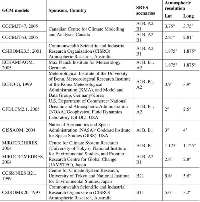
A total of 27 scenarios from 11 AOGCMs, each with two to three emission scenarios (Nakicenovic et al, 2000) are selected for developing future scenarios. Full descriptions of the emissions scenarios and AOGCMs can be found in Appendices B and C. Table 2 provides a complete list of the details of the AOGCM scenarios used in this study.

Table 2: List of AOGCM Models and Emission Scenarios

GCM models Sponsors, Country SRES

scenarios

Atmospheric resolution Lat Long

CGCM3T47, 2005

Canadian Centre for Climate Modelling and Analysis, Canada

A1B, A2,

B1 3.75° 3.75°

CGCM3T63, 2005 A1B, A2,

B1 2.81° 2.81°

CSIROMK3.5, 2001

Commonwealth Scientific and Industrial Research Organization (CISRO)

Atmospheric Research, Australia

A1B, A2,

B1 1.875° 1.875°

ECHAM5AOM, 2005

Max Planck Institute for Meteorology, Germany

A1B, B1,

A2 1.875° 1.875°

ECHO-G, 1999

Meteorological Institute of the University of Bonn, Meteorological Research Institute of the Korea Meteorological

Administration (KMA), and Model and Data Group, Germany/Korea

A1B, B1,

A2 3.9° 3.9°

GFDLCM2.1, 2005

U.S. Department of Commerce/ National Oceanic and Atmospheric Administration (NOAA)/Geophysical Fluid Dynamics Laboratory (GFDL), USA

A1B, B1,

A2 2° 2.5°

GISSAOM, 2004

National Aeronautics and Space

Administration (NASA)/ Goddard Institute for Space Studies (GISS), USA

A1B, B1 3° 4°

MIROC3.2HIRES, 2004

Centre for Climate System Research (University of Tokyo), National Institute for Environmental Studies, and Frontier Research Centre for Global Change (JAMSTEC), Japan A1B, B1 1.125° 1.125° MIROC3.2MEDRES, 2004 A1B, A2, B1 2.8° 2.8° CCSR/NIES B21, 1999

Centre for Climate System Research, University of Tokyo and National Institute for Environmental Studies, Japan

B21 5.6° 5.6°

CSIROMK2b, 1997

Commonwealth Scientific and Industrial Research Organization (CISRO)

Atmospheric Research, Australia

22

3.2 Development of Methodology

Figure 2 presents the schematic of the methods adopted for generating IDF curves for 2080s incorporating uncertainties from AOGCM scenario. The step by step procedures are presented below.

3.2.1 Downscaling

Stochastic weather generators simulate weather data to assist in the formulation of water resource management policies. The basic assumption for producing synthetic sequences is that the past would be representative of the future. They are essentially complex random number generators, which can be used to produce a synthetic series of data. This allows the researcher to account for natural variability when predicting the effects of climate change.

In order to reduce multi-dimensionality and collinearity associated with the large number of input variables, principal component analysis has been integrated with the weather generator. The process requires selecting appropriate principal components (PCs) that will adequately represent most information of the original dataset.

The WG-PCA algorithm with p variables and q stations works through the following steps:

1) Regional means of p variables for all q stations are calculated for each day of the observed data:



X t







23

Figure 2: Schematic Diagram of Developing IDF Curve

where







Modified Daily Output (27 Scenarios)

Daily Outputs 2080s (27 Scenarios)

Hourly Output 2080s (27 Scenarios)

Max. Rainfall for Diff. Durations 2080s

(27 Scenarios)

IDF Curves for 2080s (27 Scenarios) IDF Curve 2080s (Resultant Scenario) Perturbed Unperturbed Disaggregation AMS Weather Generator Cross-Correlation Analysis Regression Analysis Station Selection Observed Rainfall (Daily) Selected Observed Rainfall (Daily) Simulated Output (Present) Simulated Hourly Output (Present) Maximum Rainfall for Different Durations (Present)

IDF Curve for Present

24

2) Selection of potential neighbors, L days long where L=(w+1)  (N-1) for each of p individual variable with N years of historic record, and a temporal window of size w which can be set by the user of the weather generator. The days within the given window are all potential neighbors to the feature vector. N data which correspond to the current day are deleted from the potential neighbors so the value of the current day is not repeated.

3) Regional means of the potential neighbors are calculated for each day at all q stations.

4) A covariance matrix, Ct of size L p is computed for day t.

5) The first time step value is randomly selected for each of p variables from all current day values in the historic record.

6) Next, using the variance explained by the principal component, Mahalanobis distance is calculated with equation 3.





d_k  _t  _k k 





Where PCt is the value of the current day and PCk is the nearest neighbor transferred by the

Eigen vector. The variance of the first principle component is Var(PC) for all K nearest neighbors.

7) The selection of the number of nearest neighbors, K, out of L potential values using K  L.

8) The Mahalanobis distance dkis put in order of smallest to largest, and the first K neighbors in

the sorted list are selected (the K Nearest Neighbors). A discrete probability distribution is used which weights closer neighbors highest in order to resample out of the set of K neighbors. Using equations 4 and 5, the weights, w, are calculated for each k neighbor.

25







Cumulative probabilities, pj, are given by:



9) A random number u (0,1) is generated and compared to the cumulative probability calculated above in order to select the current day’s nearest neighbor. If p1 < u < pk, then day j

for which u is closest to pj is selected. However, if pi > u, then the day which corresponds to d1

is chosen. If u=pK, then the day which corresponds to day dK is selected. Upon selecting the

nearest neighbor, the K-NN algorithm chooses the weather of the selected day for all stations in order to preserve spatial correlation in the data (Eum et al, 2009).

10) In order to generate values outside the observed range, perturbation is used. A conditional standard deviation for K nearest neighbors is estimated. For choosing the optimal bandwidth of a Gaussian distribution function that minimizes the asymptotic mean integrated square error (AMISE), Sharma et al. (1997) reduced Silverman’s (Silverman 1986, pp. 86-87) equation of optimal bandwidth into the following form for a univariate case:

5 / 1 06 . 1   K  (3.6)

Using the mean value of the weather variablex_ij,_tobtained in step 9 and variance

2 ) (_ij , a new value y_ij_,tcan be achieved through perturbation (Sharma et al. 1997).

t j i j t i j t i x z y_,  _,  (3.7)

26

Where z_t is a random variable, distributed normally (zero mean, unit variance) for day t. Negative values are prevented from being produced for precipitation by employing a largest acceptable bandwidth: _a x*,j_t /1.55*j where * refers to precipitation. If again a negative value

is returned, a new value for ztis generated (Sharif and Burn, 2006).

3.2.2 Bias Correction of Downscaled Outputs

The downscaling process scales down coarse grid outputs of AOGCMs into the scale of interest. However, significant simulation bias still may exist from the initializations of atmospheric-oceanic processes. Hence, employing coarse resolution global model output for regional and local climate studies requires an additional bias correction step based on the ability of the AOGCMs to reproduce the past climate. In this study, bias from the downscaled outputs is corrected by the following equation:

Bias in AOGCM,

(3.8)

Where,

bi = bias from different AOGCMs

xi = Monthly mean of observed precipitation for 1965-1990 yi = Monthly mean from different AOGCMs for 1965-1990

the correction factor for the AOGCMs is then calculated using,

(3.9)

So, the treated downscaled rainfall for 2080s,

27

where,

pi = untreated daily downscaled rainfall for 2080s

3.2.3 Disaggregation

The disaggregation scheme works by extracting rainfall event records from the hourly observed data. A rainfall event can be defined as a period of non-zero rainfall for two or more days where the total amount of rainfall during the consecutive days is considered as the event rainfall value. Once the rainfall events are extracted from the historic record, they are disaggregated by a K-nearest neighbor approach. The algorithm considers daily rainfall produced by the weather generator for day , for each station. A set of potential events are selected from the observed record from which once such event is chosen based on which the daily output is disaggregated into hourly values.

The selection of neighboring events from the observed record follows simple rule:

Only events within a moving window of days are selected to account for the seasonally varied temporal distribution of rainfall. Events are selected from the prescribed moving window from all years in the historic record of events as a potential set of neighbors. The daily totals from downscaled outputs are compared with the set of neighboring event totals to assure that the only disaggregation of similar events is considered.

Observed hourly data is used as a template on how the hourly values of the generated outputs would look like. A specific number of days are considered to compare with the present day value. The best match is determined by (Mansour and Burn, 2010):

28

Where, is the daily rainfall output from weather generator, is the historical observed daily rainfall, and are the events calculated from WG outputs and historical observed data respectively. The weights are used to identify the best historical hourly ratio of the data. An hourly value set within the moving window of days can be chosen for a similar event or for the daily total rainfall . The combination of the weights, which provide the lowest for each value within the window, is considered as the daily ratio of historical hourly values used to disaggregate the WG’s daily data into hourly values. The ratio of the hourly values found within the chosen day is applied to the daily value to create a plausible hourly set-up for the given daily data. This is done based on the methods of fragments (Svanidze, 1977; Sharif et al., 2007). The fragments represent the fraction of daily rainfall that occur during each hour of the day summing to unity and can be expressed as:

∑ (3.12)

where represents the fragments calculated for hour , is the chosen hourly data from observations, is the number of hours in a day which is 24. The fragments are then multiplied with the daily data to produce data for each hour:

(3.13)

where is the daily rainfall (mm). This program has been sent daily data that already had known hourly values and the results have been compared in an attempt to verify that the model works correctly.

29

This approach utilizes locally observed data using a non-parametric method avoiding the chance of errors that may occur from the parametric methods due to theoretical distribution fits, parameter estimations and calibration. Additionally, there is high likelihood that the statistical characteristics of the disggregated rainfall are stored by applying the resampling algorithm.

3.2.4 Generation of Rainfall for Different Durations

Sampling of rainfall data for estimating rainfall extremes are commonly proceeded using two approaches: the annual maxima series (AMS) or block maxima and peak over threshold (POT) or partial duration series (PDS) (Coles, 2001). Literatures have identified limitations and advantages of both methods. Madsen et al. (1997), Buishand et al. (1990), Rasmussen et al. (1994) found POT to be a better approach than AMS. While Kartz et al. (2002), Smith (2003), de Michele and Salvadori (2005) suggested use of both methods. By definition, AMS approach includes the yearly peaks in the observational period while the POT involves all the peak events that exceed a given threshold value. The AMS method is more straightforward. If the number of annual maxima is small (<100), the obtained estimates may be sensitive to outliers. It is an asymptotic method that works well if the number of inputs from which a maximum is considered, is large. Jeruskova et al., 2006 showed that convergence to limit any distribution fit can be slow. For determining annual maxima, the maxima of 365 daily values are considered. The seasonal effect may also play a role. Application of POT is somewhat difficult than the AMS because of it’s selection of an appropriate threshold. For a satisfactory stability of the obtained results, testing of several threshold values such as 90%, 95% and 98% are recommended. Jeruskova et al. (2006) have shown that the POT method may work well for short memory series only. For longer data series, the series should be split into several more homogeneous groups. Both methods however, have their own disadvantages too; the AMS may

30

neglect certain high values, while the POT may suffer from serial correlation problem (Jervis et al., 1936; Langbein, 1949;, Taesombat and Yevjevich, 1978).

3.2.5 Intensity-Duration-Frequency Analysis

Rainfall intensity-duration-frequency (IDF) curves are derived from the statistical analysis of rainfall events over a period over time and used to capture important characteristics of point rainfall for shorter durations. It is considered as a convenient tool for gathering regional rainfall information required for municipal storm water management works. Site specific curves represent intensity-time relationship for a specific return period from a series of storms. Information is summarized by plotting the durations on the horizontal axis, the rate of rainfall (intensity in depth per unit of time) on the vertical axis and the curves for each design storm return period. Frequency is expressed in terms of return period, T, the average length of time between rainfall events that equals or exceed any given magnitude. For each selected duration, annual maximum rainfall is extracted from the rainfall data and frequency analysis is performed to the annual maximum rainfall to fit a probability distribution for standardizing the characteristics of rainfall for each station with varying rainfall record.

In Canada, Environment Canada is responsible (a) for collection and quality control of rainfall data and (b) for providing the rainfall extreme information in the form of IDF curves. Gumbel’s Extreme Value distribution is normally used to fit the annual extremes of rainfall using AMS method. It is acknowledged here that due to changes in future precipitation extremes, the future rainfall may not follow the conventionally used Gumbel’s distribution. It would be adequate to consider a generalized extreme value (GEV) distribution. But the inherent uncertainties in the responses of AOGCM outputs do not guarantee GEV as the best fit for all AOGCMs. Furthermore, fitting of three parameters for the GEV distribution by maximum

31

likelihood method requires considerable computation time, and will be different for different AOGCM responses. For simplification, and to comply with Environment Canada’s procedure, use of Extreme Value (EV) type 1 which is Gumbel distribution is adopted in this study.

The Gumbel probability distribution is expressed (Watt et al., 1989):

(3.14)

where represents the magnitude of the year event, and are the mean and standard deviation of the annual maximum series, and is a frequency factor depending on the return

period, . The frequency factor is obtained using the following equation:

√ _{( (}

)) (3.15)

Meteorological Service of Canada (MSC) uses the above method to calculate rainfall frequency for durations of 5, 10, 30 minutes and 1, 2, 6. 12, 24 hours. Since most of the stations do not have observed sub-hourly data, the calculation of the frequencies for periods shorter than 1 hour may be based on the ratios provided by the World Meteorological Organization (MTO, 1997):

Duration (min) 5 10 15 30

Ratio (n-min to 60-min) 0.29 0.45 0.57 0.79

32

The IDF data is next fitted to a continuous function in order to make the process of IDF data interpolation more efficient i.e. if the ratio of any duration is not available, the IDF data is fitted to the following three parameter function:

where presents the rainfall intensity in mm/hr, is the duration of rainfall in minute, are the constants. To obtain optimal values for these three parameters, a reasonable

value of is assumed and the values of are estimated by the least square method. The process is repeated to achieve the closest fit of the data (MTO, 1997). Plots of rainfall intensity vs. duration for each return period is then produced from the fitted IDF data to equation 3.14.

3.2.6 Uncertainty Quantification

A practical approach to deal with AOGCM and scenario uncertainties originating from inadequate information and incomplete knowledge should: (i) be robust with respect to model choice; (ii) be statistically consistent in a uniform application across different spatial scales such as global, regional or local/watershed scales; (iii) be flexible enough to deal with the variety of data; (iv) obtain the maximum information from the sample; and (v) lead to consistent results. Most parametric methods do not meet all these requirements.

Probability Density Function (PDF) is commonly used to describe the nature of data. In applications an estimate of the unknown ( ) based on random sample from ( ) is calculate in the form of ̂ ̂( ). Probability distribution functions estimated by any nonparametric method without prior assumptions can be suitable to quantify AOGCM and scenario uncertainties. Several approaches such as kernel methods, orthogonal series methods,

33

penalized-likelihood methods, k-nearest neighbor methods, Bayesian-spline methods, and maximum-likelihood or histogram like methods can be found in the literature (Adamowski, 1985).

Kernel density estimation method has been widely used as a viable and flexible alternative to parametric methods in hydrology (Sharma et al., 1997; Lall, 1995), flood frequency analysis (Lall et al., 1993; Adamowski, 1985), and precipitation resampling (Lall et al., 1996) for estimating probability density function.

A kernel density estimate is formed through the convolution of kernels or weight functions centered at the empirical frequency distribution of the data. A kernel density estimator involves the use of kernel function (K(x)) defined by:

∫ ( ) (3.17)

A PDF thus, can be used as a kernel function. The Parzen-Rosenbalt kernel density estimate ( ) at x, from a sample of { } of sample size n can is given by:

̂ ( ) ∑ ( ) (3.18)

where ( ) and ( ) is a weight or kernel function required to satisfy criteria such as

symmetry, finite variance, and integrates to unity. Successful application of any kernel density estimation depends more on the choice of the smoothing parameter or bandwidth (h) and the type of kernel function K(.), to a lesser extent. Bandwidth for kernel estimation may be evaluated by minimizing the deviation of the estimated PDF from the actual one.

34

The behavior of the estimator (equation 3.18) may be analyzed mathematically under the assumption that the data sets represent independent realizations from a probability density f(x). The basic methodology of the theoretical treatment is to discuss the closeness of estimator ̂ to the true density, . Successful application of the estimator depends mostly on the choice of a kernel and a smoothing parameter or bandwidth. Literatures have found that the choice of bandwidth is more critical. A change in kernel bandwidth can dramatically change the shape of the kernel estimate (Efromovich, 1999). For each x, ̂( ) can be thought as a random variable because of it’s dependence on . Except otherwise stated, ∑ will refer to a sum for and ∫ to an integral over the range ( ).

The discrepancy of the density estimator ̂ from it’s true density can be measured by mean square error (MSE):

( ̂) ( ̂( ) ( ) (3.19)

By standard elementary properties of mean and variance,

( ̂) { ( ̂( ) ( ) } ̂( ), (3.20)

the sum of the squared bias and the variance at . In many applications a trade-off is applied between the bias and the variance in equation (3.20); the bias can be reduced by increasing the variance and vice versa by adjusting the degree of smoothing.

It can be obtained by minimizing the mean integrated square error (MISE), a widely used measure of global accuracy of ̂ as an estimator of (Rosenblatt, 1956; Adamowski, 1985; Scott et al., 1981, Jones et al., 1996) defined as:

35

( ̂) ∫ ( ̂( ) ( ) (3.21)

or in alternative forms,

( ̂) ∫ ( ̂)

∫ ( ̂( ) ( ) ∫ ( ̂) (3.22)

which gives the as the sum of the integrated square bias and the integrated variance.

Asymptotic analysis provides a simple way of quantifying how the bandwidth h works as a smoothing parameter. Under standard assumptions, MISE is approximated by the asymptotic mean integrated square error (AIMSE) (Jones et al., 1996):

( ) _{( ) ( )(∫ ⁄ ) (3.23)}

where ( ) ∫ ( ) and∫ ∫ ( ) , n is sample size, h is bandwidth. The first term (integrated variance) is large when h is too small, and the second term (integrated squared bias) is large when h is too large.

The minimizer of ( ) is easily calculated as:

( ) [

( )(∫ )

]

(3.24)

In this study the solve-the-equation-plug-in approach is used to derive the data-driven bandwidth for estimating the densities.

The main thought behind the ‘solve the equation plug in’ approach is to plug an estimate of the unknown ( ) in the equation (3.24). The major challenge is to estimate a pilot bandwidth.

36

The ‘solve the equation’ approach proposed by Hall (1980), Sheather (1983, 1986) and later refined by Sheather and Jones (1991) is used in this study. The smallest bandwidth, hSJPI is

considered as the solution of the fixed point equation

[

( ̂ _{( )})(∫ )

]

A dummy minimizer in the form g(h) is used to provide better representation of ( ). It is done by estimating an analogue of for estimating ( ) by ( ̂ ).

The minimizer of the asymptotic mean square error (AMSE) is expressed as:

{ ( )} ( )

(3.26)

for suitable functional and . The expression of in terms of comes from solving the representation of for and substituting to get

( ) { ( _{) ( )} ( ) (3.27)}

for appropriate functionals , . The unknowns ( ) and ( ) are estimated by ( ̂ ) and ( ̂ _{), with bandwidths chosen by reference to a parametric family, as for}

.

Many variations have been tested for treatment of ( ̂ ) and ( ̂ ).The major contribution has been to try to reduce the influence of the normal parametric family even further by using pilot kernel estimates instead of normal interference (Jones et al., 1996). Park and Marron (1990) has shown the improvements in terms of the asymptotic rate of convergence up to a certain point.

37

4. Results and Discussion

This chapter presents the results of the methodology introduced above for the development of IDF curve for 2080s. Results are presented for the City of London.

4.1 Selection of Appropriate Stations

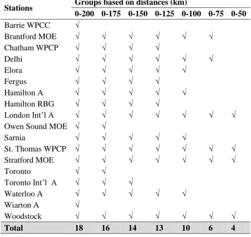
The number of stations used to generated long sequence of rainfall series influence outputs of weather generator. Stations surrounding the point of interest help to capture the spatial and temporal characteristics in the region. In cases where only limited data is available, surrounding stations may help to add spatial and temporal characteristics of the rainfall values. Conversely, use of too many stations can be computationally expensive and unnecessary; especially for short duration rainfall where convective storms are highly localized weather patterns, operating on relatively small spatial scales. Stations located too far may affect the performance of weather generator. So regression and cross correlation analysis are performed for identifying important stations for London. For regression analysis, the stations are grouped based on selected distances from London (Table 3). Regression results for each group are provided in the Appendix A. The results are expressed in terms of t-test statistics, p values and the coefficient of determination.

Results from the Appendix A show significant t-test statistic for all predictors reducing the possibility of over-fitting by an insignificant predictor. The term ‘probability value’ (p) denotes the results of the testing of hypothesis that the regression coefficient is equal to zero which in turn quantifies the importance of the regressor. A result of α in the probability value column for a predictor X denotes that with (100) X (1- α)% of confidence one can reject the hypothesis that

38

the coefficient of predictor X is zero. Low or near zero value of α is desirable as it is inversely related to the importance of a predictor.

Table 3: Groups for Regression Analysis based on Distances

Stations Groups based on distances (km)

0-200 0-175 0-150 0-125 0-100 0-75 0-50 Barrie WPCC √ Brantford MOE √ √ √ √ √ √ Chatham WPCP √ √ √ √ Delhi √ √ √ √ √ √ Elora √ √ √ √ √ Fergus √ √ √ √ Hamilton A √ √ √ √ √ Hamilton RBG √ √ √ √ London Int’l A √ √ √ √ √ √ √

Owen Sound MOE √ √

Sarnia √ √ √ √ √ St. Thomas WPCP √ √ √ √ √ √ √ Stratford MOE √ √ √ √ √ √ √ Toronto √ √ Toronto Int’l A √ √ √ Waterloo A √ √ √ √ √ Wiarton A √ Woodstock √ √ √ √ √ √ √ Total 18 16 14 13 10 6 4

The t-statistics for the independent variables are equal to their coefficient estimates divided by their respective standard errors. In theory, the t-statistic of any one variable may be used to test the hypothesis that the true value of the coefficient is zero (which is to say, the variable should not be included in the model). In a standard normal distribution, only 5% of the values fall outside the range plus-or-minus 2 A low t-statistic (or equivalently, a moderate-to-large exceedance probability) for a variable suggests that the SEE would not be adversely affected by its removal. The rule-of-thumb in this regard is to remove the least important variable if its t-statistic is less than 2 in absolute value, and/or the exceedance probability is greater than .05

39

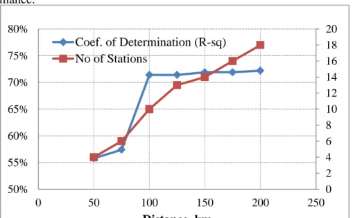
(Minitab help, 2009). From the results it is seen that stations within 100 km distances appear to be the best option for London. This can be clearly seen from the coefficient of determination plot in Figure 3 where addition of more stations, beyond 100 km distance apparently cannot improve the model performance.

Figure 3: Performances of Stations based on Distance

Next, the cross correlation analysis is performed to identify the correlation between the stations (Table 4). Results show that stations within 100 km radius are correlated well, with correlation greater than 60% for all stations but Elora. However, the regression test shows that inclusion of Elora may provide important information to the spatial and temporal pattern of London. So it is included for IDF analysis. So finally, nine stations with hourly and daily rainfall data from 1965-2001, located within 100 km radius of London station have been selected for further analysis.

Both historical daily and hourly data contains missing values. Inverse distance weighted methods is applied to fill the missing values.

0 2 4 6 8 10 12 14 16 18 20 50% 55% 60% 65% 70% 75% 80% 0 50 100 150 200 250 Distance, km Coef. of Determination (R-sq) No of Stations

40

Table 4: Cross-Correlation Results for Stations Within 200 km Distance from London

Stations Distance (km) Lag -2 -1 0 1 2 London A 0 -0.004 0.094 1.000 0.094 -0.004 Waterloo A 78 -0.004 0.063 0.729 0.097 0.000 Woodstock 33 0.003 0.273 0.723 0.022 -0.012 Sarnia 93 0.018 0.131 0.676 0.054 -0.014 Hamilton A 100 0.003 0.050 0.670 0.136 -0.008 Delhi CS 52 -0.004 0.236 0.657 0.020 -0.014 Brantford MOE 75 0.000 0.249 0.645 0.026 -0.019 Stratford MOE 39 -0.005 0.263 0.633 0.028 -0.004 Hamilton RBG 106 0.002 0.214 0.618 0.037 -0.008 Toronto Int’l A 142 -0.002 0.043 0.610 0.125 0.000 St. Thomas WPCP 28 -0.009 0.344 0.609 0.030 -0.008 Fergus 102 -0.005 0.203 0.564 0.033 -0.009 Toronto 158 -0.005 0.158 0.564 0.028 -0.012 Elora 91 -0.002 0.199 0.550 0.066 0.002 Chatham WPCP 113 -0.006 0.278 0.488 0.008 -0.013 Barrie 190 -0.010 0.122 0.461 0.062 -0.007 Wiarton A 190 -0.021 0.049 0.454 0.101 -0.009 Owen Sound 173 -0.024 0.146 0.373 0.047 -0.005

4.2 Development of Climate Change Scenarios

Climate change scenarios from AOGCM outputs (Table 2) are used to condition the input data using the weather generator. Outputs from AOGCMs for 1961-1990 represent baseline climate against which the future climate change scenarios for 2071-2099 (2080s) have been computed.

Based on the AOGCM data, change fields for each scenario is calculated as the difference between the monthly mean precipitation from their 1961-1990 mean.

41

This difference is then multiplied with the locally observed station data to generate climate change scenarios appropriate for the City of London at a daily time scale. As an example, if the change field for the month of July and August are 10% and -5%, all daily July and August rainfall values are multiplied by a factor of 1.05 and 0.95, respectively. This newly modified data is then used with the weather generator to generate daily time series of any preferred length for different scenarios. For this study, 27 different climate scenarios are developed which represent different realizations of future. Comparison of 1961-1990 mean historical observed rainfall with those developed from different scenarios for base climate reveal that significant bias still exit in the base climate which is used to initialize the future climate; which means the bias may be carried out in the downscaled output. Table 5 (a) presents a comparison between the monthly mean precipitation from different AOGCM scenarios and historical observed values. Mean monthly precipitation vary significantly for between months for all models.

Table 5 (a): Monthly Mean Precipitation (mm) from Different AOGCMs for 1965-1990

Scenarios/month Jan Feb Mar Apr May Jun Jul Aug Sep Oct Nov Dec Observed 2.28 2.21 2.51 2.65 2.48 2.80 2.46 2.79 3.04 2.66 3.17 3.16 CGCM3T47 1.99 1.95 2.25 2.71 2.88 2.66 2.12 2.11 2.35 2.29 2.88 2.73 CGCM3T63 2.14 1.80 2.45 2.84 3.69 3.42 3.00 2.40 2.30 2.87 2.67 2.93 CSIROMK3 1.94 2.16 2.44 2.97 3.28 2.64 2.42 1.80 1.72 2.31 2.42 2.21 ECHAM5OM 3.01 3.63 3.62 4.11 4.33 4.41 3.58 3.47 3.32 2.47 2.99 3.09 ECHO-G 2.08 2.10 2.49 3.43 4.45 3.66 3.82 3.18 2.59 2.67 2.92 2.21 GFDLCM2.1 2.46 2.83 2.86 2.90 3.54 3.19 3.23 3.04 3.36 2.29 2.83 2.62 GISSAOM 2.04 2.22 2.51 2.79 2.54 2.21 2.59 2.91 3.18 3.04 2.57 2.56 MIROC3.2_HIRES 2.88 2.56 2.97 3.32 3.01 3.23 3.76 3.34 3.40 2.90 3.28 3.14 MIROC3.2_MEDRES 2.21 2.57 2.64 2.86 2.92 3.49 3.71 3.00 2.96 2.47 2.52 2.40 CCSRNIES_B21 1.84 2.24 2.86 3.25 3.63 4.18 4.77 3.52 2.07 1.40 1.73 2.05 CSIROMk2b_B11 1.51 1.53 1.74 2.34 2.50 3.21 3.26 2.20 1.71 1.88 1.79 1.64

4.3 Verification of the IDF Generation Methods

42

used to simulate a sequence of rainfall for all stations. For the verification purpose, the perturbation of the weather generator described in section 3.3.1 is kept off in order to replicate the exact scenario as the historical, observed, one.

This study uses 10 stations for the period of 1965-2003 (N=39) to simulate different rainfall scenarios. Employing the temporal window of 14 days (w=14) and 39 years of historic data (N=39), 584 days are considered as potential neighbors (L=(w+1) x N-1=584). Each case is simulated three times thus generating 117 years of simulated output. It is expected that such length of output is sufficient enough to estimate event with return period of 100 years.

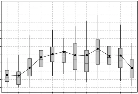
In order to test the output of the weather generator, the box and whisker plots for monthly historical simulated rainfall are created (Figure 4).

Figure 4: Box and Whiskers Plot of Simulated Monthly Rainfall in London

The boxes show the 25th percentile, 50 percentile and 75th percentiles of data while the whiskers, plotted with 1.5 times the inter-quartile range from the boxes. For all cases historic

Dec Nov Oct Sep Aug Jul Jun May Apr Mar Feb Jan 200 180 160 140 120 100 80 60 40 20 0 M o n th ly R a in fa ll ( m m )

43

observed means are shown in terms of line plot to assess the ability of the weather generator to reproduce the temporal and spatial character of rainfall for the City of London. From the Figure 4, it is seen that the model has been able to replicate the historic observed pattern adequately.

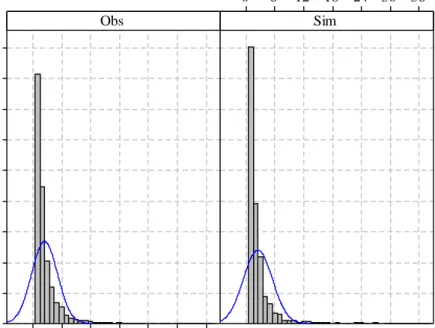
Next, the daily rainfall is disaggregated into hourly values using the method described in section 3.2.3. The comparison of the performance of the historic simulated hourly values with the observed hourly data is presented in terms of frequency plots (Figure 5).

Figure 5: Frequency Plots of Observed (Obs) and Simulated (Sim) Hourly Rainfall

The frequency of small range rainfall is slightly over-estimated and the mid range rainfall is slightly under-estimated by the disaggregation model. Overall, the frequency of the extreme rainfall is captured well.

Finally, the annual maximum rainfall for 1, 2, 6, 12 and 24 hour durations is generated to fit Gumbel distribution for calculating return periods. These are then compared with the IDF information obtained from Environment Canada (EC) (Table 6). It should be noted that the

36 30 24 18 12 6 0 900 800 700 600 500 400 300 200 100 0 36 30 24 18 12 6 0 Obs

Hourly Pre cipitation (mm)

F re q u e n c y Sim

44

Environment Canada uses rainfall data from 1943-2001 to develop IDF curves for London. However, hourly data is available only from 1961; data prior to 1961 may exist in paper form and are not available. For the present study, the hourly rainfall data for London is further reduced down to 1965 for matching rainfall data from other nearby stations to be used for multi-site weather generator.

Table 6 (a): Comparison of Extreme Rainfall in London in terms of Depth (mm) Historic Unperturbed (1965-2003) Return Period, T years

Duration, hrs 2 5 10 25 50 100 1 21.80 30.38 36.06 43.24 48.56 53.85 2 28.05 40.11 48.09 58.18 65.66 73.09 6 36.41 49.90 58.83 70.11 78.49 86.80 12 42.61 56.33 65.41 76.89 85.40 93.86 24 49.70 64.63 74.52 87.01 96.28 105.48

EC (1943-2003) Return Period, T years

Duration, hrs 2 5 10 25 50 100 1 24.40 35.30 42.50 51.60 58.30 65.00 2 29.60 41.60 49.50 59.60 67.00 74.40 6 36.70 48.20 55.80 65.40 72.50 79.60 12 43.00 54.70 62.50 72.40 79.70 87.00 24 51.30 66.80 77.10 90.00 99.60 109.20

Table 6 (a) presents the intensity-duration-frequency data obtained from the historic unperturbed scenario together with the IDF data generated by EC. The results obtained are compared in terms of the relative differences using the following relationship:

| | (3.28)

45

Table 6 (b) presents the relative difference of rainfall intensity between the historic unperturbed and the EC data. The short duration rainfall (1 hr) is underestimated by the historic unperturbed scenario, while the intermediate (2, 6, 12 hrs) and longer (24 hrs) duration rainfalls are able to closely replicate the EC generated intensities for all return periods. Overall, the performance of the historic unperturbed scenario is satisfactory.

Table 6 (b): Relative Difference between EC IDF Information and Historic Unperturbed Scenario

Duration, min Return Period, years

2 5 10 25 50 100 60 11.25 14.98 16.39 17.63 18.22 18.76 120 5.38 3.66 2.89 2.42 2.02 1.78 360 0.80 3.46 5.29 6.96 7.93 8.65 720 0.91 2.94 4.56 6.02 6.91 7.58 1440 3.18 3.30 3.40 3.37 3.39 3.46

4.4 IDF Results for Future Climate

The perturbation process inside the weather generator is added (described in section 3.2.1) to generate IDF information using the historical observed rainfall. This scenario called ‘historical perturbed’ assumes that the future climate will continue to change as the consequence of already altered green house gas concentrations in the atmosphere, ignoring any future change in green house gas emissions.

The daily weather generator output, after being disaggregated into hourly rainfall, is next used to generate intensity duration frequency data for 27 different scenarios presented in Table 4

46

to create different realizations of future climate using different AOGCM responses. Appendix D presents the IDF data obtained using climate scenarios in terms of intensity.

The difference in the AOGCM scenarios relative to the historic perturbed scenario is summarized in Table 7.

Table 7: Percent Differences between Historic Perturbed, Wet and Dry Scenarios ECHAM5AOM_A1B (Wet Scenario) and Historic Perturbed

Duration, min

Return Period, years

2 5 10 25 50 100 60 62.68 69.56 72.42 75.00 76.44 77.60 120 60.64 65.84 67.98 69.91 70.99 71.86 360 65.13 77.09 82.29 87.12 89.88 92.13 720 66.03 77.77 83.09 88.17 91.13 93.57 1440 63.22 72.99 77.42 81.63 84.07 86.09

MIROC3MEDRES_A2 (Dry Scenario) and Historic Perturbed

Duration, min

Return Periods, years

2 5 10 25 50 100 60 -6.79 -2.90 -1.28 0.18 0.99 1.65 120 -12.70 -15.09 -16.07 -16.96 -17.45 -17.85 360 -7.06 -6.60 -6.40 -6.21 -6.10 -6.02 720 -0.68 1.66 2.72 3.73 4.32 4.81 1440 -0.44 -0.10 0.05 0.20 0.28 0.35

The model results show variable results, with wide range of increase in extreme rainfall. ECHAM5AOM A1B appears to be the wettest while MIROC3.2MEDRES A2 being the driest of all. The wettest ECHAM5AOM A1B model shows more than 60% increase in rainfall compared to historic perturbed scenario. While the driest MIROC3.2 MEDRES A2 scenario shows slight decrease in precipitation intensity than the historic perturbed scenario. The difference between the wettest and the driest scenario ranges from 70% to 92% indicating huge range of uncertainty

47

among the realizations of AOGCMs. A comparison of different AOGCMs for specific duration is presented in Figure 6.

48

Figure 6: IDF Plots of AOGCM Scenarios for Different Durations

20 40 60 80 100 120 0 20 40 60 80 100 120 De p th, m m

1 hr

6 hr

2 hr

Return Period, yrs

24 hr

Return Period, yrs

12 hr

49

4.5 Uncertainty Quantification of IDF Results

Becaus