HAL Id: hal-01272125
https://hal.archives-ouvertes.fr/hal-01272125
Submitted on 10 Feb 2016HAL is a multi-disciplinary open access archive for the deposit and dissemination of sci-entific research documents, whether they are pub-lished or not. The documents may come from teaching and research institutions in France or
L’archive ouverte pluridisciplinaire HAL, est destinée au dépôt et à la diffusion de documents scientifiques de niveau recherche, publiés ou non, émanant des établissements d’enseignement et de recherche français ou étrangers, des laboratoires
Sunlab: a Functional-Structural Model for Genotypic
and Phenotypic Characterization of the Sunflower Crop
Fenni Kang, Paul-Henry Cournede, Jeremie Lecoeur, Véronique Letort
To cite this version:
Fenni Kang, Paul-Henry Cournede, Jeremie Lecoeur, Véronique Letort. Sunlab: a Functional-Structural Model for Genotypic and Phenotypic Characterization of the Sunflower Crop. Ecological Modelling, Elsevier, 2014, 290, pp.21-33. �10.1016/j.ecolmodel.2014.02.006�. �hal-01272125�
Sunlab: a Functional-Structural Model for Genotypic
1and Phenotypic Characterization of the Sunflower Crop
2Fenni Kanga, Paul-Henry Cournedea, Jeremie Lecoeurb, Veronique 3
Letorta,∗
4
aLaboratory MAS, Ecole Centrale Paris, Grande Voie des Vignes, F-92 295
5
Chatenay-Malabry, France 6
bMontpellier SupAgro, 2, Place Pierre Viala, 34060 Montpellier Cedex 2
7
Abstract
8
A new functional-structural model SUNLAB for the crop sunflower ( He-lianthus annuus L.) was developed. It is dedicated to simulate the sunflower organogenesis, morphogenesis, biomass accumulation and biomass partition-ing to organs. It is adapted to model phenotypic responses of different genotypic variants to diverse environmental factors including temperature stress and water deficit. A sensitivity analysis was conducted to quantify the relative parameter influences on the main trait of interest, the grain yield. The model was calibrated for four genotypes on two experimental datasets collected on plants grown under standard non-limiting conditions and mod-erate water stress. Its predictive ability was then tested on an additional dataset. The four considered genotypes - “Albena”, “Melody”, “Heliasol” and “Prodisol” - are the products of more than 30 years of breeding ef-fort. Comparing the values found for the four parameter sets associated to each variant, allows to identify genotype-specific parameters. The model also provides a novel way of investigating genotype performances under different environmental conditions. These promising results are a first step towards
the potential use of the model as a support tool to design sunflower ideotypes adapted to the current worldwide ecological and economical challenges and to assist the breeding procedure.
Keywords: SUNLAB, SUNFLO, GREENLAB, Sunflower model 9
1. Introduction
10
As one of the major oilseed crops worldwide, sunflower production has 11
to face the growing social demand in a context of strong ecological and eco-12
nomical constraints: growers are confronted to the challenge of increasing 13
sunflower productivity under changing climatic conditions while maintaining 14
low input levels and reduced costs. A partial response to this challenge could 15
be found by breeding new genotypes or by identifying the best genotype, 16
among a set of existing ones, for a given location and for given management 17
practices; see for instance Allinne et al. (2009). 18
Assessments of genotype performances forin situexperimental trials ham-19
per the breeding process by temporal, logistic and economical difficulties. 20
Indeed, genotypes perform differently depending on the environmental con-21
ditions (soil, climate, etc.) and the management practices (sowing date, 22
nitrogen inputs, irrigation, etc.). Therefore a large number of trials are 23
needed to explore a sufficiently diverse set of genotypes x environment x 24
management (GxExM) combinations in order to characterize these complex 25
interactions. An emerging approach to overcome these difficulties relies on 26
the use of models represented as a set of biophysical functions that deter-27
mine the plant phenotype in response to environmental inputs. Models can 28
help in breeding strategies and management by dissecting physiological traits 29
into their constitutive components and thus allow shifting from highly inte-30
grated traits to more gene-related traits that should reveal more stable under 31
varying environmental conditions (Yin et al., 2004; Hammer et al., 2006). 32
Consequently, an important question to examine is how to design models 33
that can be used in that context. The models should simulate the phenotypic 34
traits of interest (e.g. yield) with good robustness and predictive capacity. 35
The models should also present a trade-off between mechanistic aspect and 36
complexity: Chapman et al. (2003) state that, for such use, a growth model 37
should include ‘principles of response and feedbacks’ to ‘handle perturbations 38
to any process and self-correct, as do plants under hormonal control when 39
growing in the field’ and to ‘express complex behavior even given simple op-40
erational rules at a functional crop physiological level’. Casadebaig et al. 41
(2011) discuss that question in the case of their model SUNFLO (Lecoeur 42
et al., 2011). SUNFLO is a biophysical plant model that describes organo-43
genesis, morphogenesis, and metabolism of sunflower (Helianthus annuus L.). 44
It has shown good performances to identify, quantify, and model phenotypic 45
variability of sunflower at the individual level in response to the main abi-46
otic stresses occurring at field level but also in the expression of genotypic 47
variability (Casadebaig et al., 2011). The authors mixed mechanistic and sta-48
tistical approaches to deal with highly integrative variables such as harvest 49
index (HI). This HI factor is determined by a simple statistical relation-50
ship dependent on covariables previously simulated by the mechanistic part 51
of the crop model throughout the growing season. Although this statistical 52
solution and the large datasets used for its parameterization conferred good 53
robustness to the prediction of HI and thereby crop harvest, biomass parti-54
tioning to other plant organs and trophic competition between organs were 55
not taken into account. Fenni: Here, in last review, the third reviewer posed
56
a question “ The idea of formalizing trophic competition between organs (p 4
57
l 27-33) is at the core of this new model. You write that such a formalization
58
should help representing feedback effects of biomass partitioning on “other
59
processes” (p 4 l 13-15). What do you mean?”, I simply deleted the sentence
60
that saying “feedback effects of biomass partitioning on other processes
can-61
not be taken into account”, but I still tried to mention it in the discussion
62
saying “The plants are considered only at the minimal level of organ
com-63
partments. PBM model ignores plant architecture and its plasticity. The
64
lack of individual organ’s simulation can influence the simulation of plant
65
functioning. For example, PBMs models normally use the relative values of
66
the sink strength of organs to simulate biomass partitioning. These sink
val-67
ues are assessed directly from experiments and the sources and sinks have no
68
significant direct interaction in these models (de Reffye et al., 2008).
How-69
ever, the lack of trophic competition simulation may hinder the simulation of
70
feedback effects of biomass partitioning on other processes. As Pallas et al.
71
(2008) state, trophic competition influenced the organogenesis of grapevine
72
in their research”. That paragraph had been deleted by you in last revision.
73
Do you think we should still mention somewhere this idea “mechanistic
sink-74
source solver helps the simulation of biomass partitioning, and also the future
75
possibility of simulating feedback effects”?. I added one sentence in the dis-76
cussion to add about considering feedback effects:”’Introducing a mechanism 77
of trophic competition at organ level in a PBM, as done in this study, opens 78
the possibility to model feedbacks effects of biomass partitioning on other 79
processes such as photosynthesis or organogenesis (Mathieu et al., 2009). 80
”‘. Do you agree? Moreover, it was shown in Lecoeur et al. (2011) that 81
HI is the parameter that contributes the most (14.3%) to the coefficient of 82
variation of the potential grain yield. It was also shown that when ranking 83
the processes in terms of their impact on yield variability, the first one was 84
biomass allocation (before light interception according to plant architecture, 85
plant phenology and photosynthesis). Therefore, Lecoeur et al. (2011) sug-86
gested that a better formalisation of the trophic competition between organs 87
could be a way to improve our understanding of genotypic variation for the 88
harvest index Fenni: here the third reviewer posed another question last
89
time “ Please elaborate and give appropriate references to clarify the idea of
90
formalizing trophic competition (direct formalization? It could also be
indi-91
rect) and to construct a sound argument (e.g. which outlines to satisfy the
92
need of feedback effects of biomass partitioning).” I actually didn’t answer
93
his question about direct formalization or indirectIn fact I don’t understand 94
the reviewer’s question; what do you think he means by ”‘direct or indi-95
rect formalization”’ ?. In order to take up this challenge, a new sunflower 96
model, named SUNLAB, was derived from SUNFLO. The representation 97
of plant topological development and allocation process at individual organ 98
scale were inspired by the functional-structural plant model GREENLAB, 99
which has been designed as a “source-sink solver” (Christophe et al., 2008) 100
and which is accompanied with the appropriate mathematical tools for its 101
identification (Cournede et al., 2011). SUNLAB thus inherits from GREEN-102
LAB the flexible rules of sink competition for biomass partitioning at organ 103
scale Fenni:the deleted phrases “(organ type includes blade, petiole,
ode and capitulum; a leaf consists of a blade and a petiole; for the modeling
105
of trophic competition, blade and petiole are considered as two organ types)”
106
were actually trying to answer the second reviewer’s question in the previous
107
review “ you are using the word “blade” to designate the leaves all over the
108
manuscript. This is somewhere confusing. The manuscript would benefit to
109
clarify this”. Maybe somewhere a small explanation of blade could be added
110
if it is deleted hereYes, I had taken care of that and I had added it in the MM 111
part, inplantstructureparagraph as ”‘ The different organ types, denoted as 112
o, include leaves (decomposed into blades and petioles),”’ Do you think that 113
it will be ok ?, together with the more detailed representation of ecophysio-114
logical processes and environmental stress effects on biomass production and 115
yield from SUNFLO. 116
This paper presents in detail the mechanisms of SUNLAB and the pa-117
rameter estimation procedure based on field experimental data. A sensitivity 118
analysis is performed on the model parameters, using the Sobol method, to 119
investigate the relative contribution of each parameter and their interac-120
tions to the model output uncertainty. The output that we consider is the 121
main trait of interest in most breeding procedures, that is the final grain 122
yield. The potentials of SUNLAB for genotypic characterization are illus-123
trated by comparing the parameters obtained after the estimation process 124
for four genotypes, namely “Albena”, “Heliasol”, “Melody” and “Prodisol”. 125
The performances of SUNLAB to reproduce phenotypic variability coming 126
either from genotypic or from environmental influences are tested against 127
experimental datasets used for parameterization. An additional dataset is 128
then used for model evaluation. An interesting and uncommon output of 129
SUNLAB is the simulation of specific leaf area (SLA, also known as leaf spe-130
cific surface area, cm2.g−1), i.e. the ratio of leaf area to dry leaf mass. It is 131
an influent input variable often associated with large uncertainty ranges in 132
most dynamic crop growth models (Rawson et al., 1987). 133
2. Materials and methods
134
2.1. Modeling: SUNLAB modules
135
SUNLAB consists of five modules: phenology, water budget, organogen-136
esis and morphogenesis, biomass accumulation, and biomass partitioning. 137
Phenology, water budget, and biomass accumulation modules are directly 138
inherited from the SUNFLO model. The organogenesis and morphogenesis 139
module is modified from the corresponding SUNFLO module by defining for 140
each organ the dates, expressed in thermal time, of initialization, termination 141
of its growth, and organ expansion. The biomass partitioning module is an 142
entirely new module. We describe here equations of these modules, briefly 143
for those inherited from SUNFLO - we refer to Casadebaig et al. (2011) and 144
Lecoeur et al. (2011) for an exhaustive description - and in detail for the 145
new contributions. Model parameters that are mentioned in the following 146
equations will be summarized in section 2.3. 147
2.1.1. Phenology
148
Plant phenology is driven by thermal time. Cumulative thermal time on 149
day d since emergence, CT T(d) (◦C days), is calculated in equation (1) as 150
the sum of the daily mean air temperature Tm(d) (◦C) above a base
tem-151
perature Tb of 4.8 ◦C, common to all sunflower genotypes. Four key
phe-152
nological stages, expressed as genotype-dependent thermal dates (◦C days), 153
are defined: flower bud appearance E1, beginning of flowering F1, begin-154
ning of grain filling M0 (early maturation) and physiological maturity M3 155
(Lecoeur et al., 2011). Crop development can be accelerated by water stress, 156
that causes overheating of the plant through the reduction of transpiration. 157
This is modeled by using a multiplicative effect of water stress at day d, 158
FHTR(d)(the effect of water on transpiration), on thermal time accumula-159 tion CT T(d): 160 Teff(d) = max(0,(Tm(d)−Tb)) CT T(d) = d X k=1 Teff(k)×[1 + 0.1×(1−F HT R(k))] (1)
where Teff(k) is the effective thermal time at day k. FHTR(d) is calculated
161
as a function of the fraction of transpirable soil water at day d, F T SW(d) 162
(detailed in 2.1.2), divided by a genotypic parameter RT of sensitivity to 163
water deficiency (Casadebaig et al. (2011)). 164
2.1.2. Water budget
165
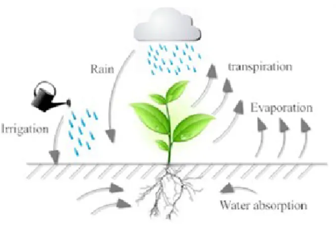
In SUNLAB, the water cycle of sunflower is modeled considering the plant 166
processes (root water absorption and transpiration), in combination with its 167
direct environment: precipitation, irrigation, soil evaporation (see Fig. 1a). 168
Evaporation and plant transpiration decrease the available amount of water 169
in soil, while irrigation and precipitation refill it. 170
[Figure 1 about here.] 171
The index for the assessment of drought levelFTSW(d) at dayddepends 172
on the simulation of the above mentionned processes (Lecoeur et al., 2011). 173
It takes values from 0 (no water stress) to 1 (severe water stress) and it is 174
used to define three indices to tune three plant functioning processes: leaf 175
expansion FHLE, radiation use efficiency FHRUE and plant transpiration 176
FHTR. The critical thresholds RT and RO are genotype-dependent pa-177
rameters varying in [0,1] that characterize the plant drought tolerance (RT, 178
drought tolerance of leaf expansion; RO, drought tolerance of radiation use 179
efficiency and transpiration). For instance, FHRUE is calculated as: 180 FHRUE(d) = FTSW(d)/RT for FTSW(d)< RT 1 for FTSW(d)≥RT (2)
Its effect on radiation use efficiency RUE(d) (g.M J−1) is defined as:
181 RU E(d) = RU Ep(d)×min 1,FTSW(d) RT ×F T(d)×P HS (3) where RUEp(d) (g.M J−1) is the crop potential (maximal) radiation use
ef-182
ficiency, F T(d) is the thermal stress on day d, a function of daily mean 183
temperature (Lecoeur et al., 2011) and PHS is a genotypic parameter giving 184
the ratio of the genotype photosynthesis capacity to that of the reference 185
genotype “Melody”. The potential radiation use efficiency is thus weakened 186
by the environmental thermal stress factor F T(d) and the drought stress 187
factor FHRUE(d). 188
2.1.3. Organogenesis and morphegenesis
189
Ecophysiological functions. The number of blades N(d) on day d increases 190
linearly with cumulative thermal time CT T(d): 191
N(d) = R×CT T(d) + 1 (4)
where R (leaves/ ( ◦Cdays)) is the rate of leaf production. Leaf senescence 192
occurs during the period of grain filling between M0 and M3. Consequently 193
the number of senescent leaves N S(d) is considered to increase in proportion 194
to the time elapsed since M0 (Sinclair and de Wit, 1975; Nooden et al., 1997) 195 as: 196 N S(d) = Ntotal × M3−CT T(d) M3−M0 (5)
whereNtotal is a genotypic parameter equal to the maximal number of leaves.
197
Since, in sunflower, leaf area distribution along the stem shows a bell shape, 198
total leaf area A(d) (cm2) per plant is calculated with a logistic equation:
199
A(d) = A1
1 +e4×A3×(A2−N(d))/A1 (6)
where A1 (cm2) is the maximal leaf area, A2 and A3 (cm2) are respectively 200
the rank and the area of the largest leaf of the plant. The calculation of 201
senescent leaf area AS(d) (cm2) is determined by a similar logistic equation 202
but replacingN(d) byN S(d). The photosynthetically active leaf areaAA(d) 203
(cm2) is estimated as the difference between total leaf areaA(d) and senescent 204
leaf areaAS(d). Leaf growth and senescence are affected by water stress and 205
temperature stress coefficients as described in Casadebaig et al. (2011). 206
AA(d) = A1
1 +e4×A3×(A2−N(d))/A1 −
A1
1 +e4×A3×(A2−N S(d))/A1 (7)
Plant structure. The different organ types, denoted as o, include leaves (de-207
composed into blades and petioles), internodes and capitulum. For each 208
individual organ o at ranki (itakes its values from 0 to the total amount of 209
individual organs of type o), its emergence thermal timeinitT T(o, i), senes-210
cence thermal time seneT T(o, i), and growth expansion duration in thermal 211
time epdT T(o, i) are defined. The thermal time of blade emergence and 212
senescence are calculated through inversion of equations 4 and 5: 213 initT T(blade, i) = (i−1)/R seneT T(blade, i) =M3− i×(M3−M1) Ntotal (8)
For the calculation of blade expansion duration epdT T(blade, i), three pa-214
rameters initT T Adjust (◦C days), epdT T A (◦C days), epdT T B (◦C days) 215
are added to the module to calculate epdT T(blade, i) based on the blade 216
emergence and senescence thermal times: 217
epdT T(blade, i) = seneT T(blade, i)−(epdT T B−epdT T A×i) −(initT T(blade, i)−initT T Adjust)
(9)
Since leaf emergence was recorded when lengths of their central vein are big-218
ger than 4cm (Lecoeur et al., 2011), the leaf has already received a small 219
amount of biomass at the recorded thermal time initT T(blade, i). There-220
fore, thermal time of blade growth initialization is calculated by subtracting 221
initT T Adjust to the emergence thermal time initT T(blade, i). The thermal 222
times of end of blade expansion linearly vary with their ranks and depend 223
on two parameters, epdT T Aand epdT T B. 224
The petiole at rank i shares the same initial, senescence and expansion 225
thermal times as the blade ibelonging to the same metamer. The internode 226
i has also the same emergence thermal time as the blade i while its expan-227
sion durationepdT T(internode, i) is driven by a parameterinternodeEpdT T
228
that is common to all internodes. Capitulum initialization thermal time 229
corresponds to M0. Its expansion duration is defined by the parameter 230
capitulumEpdT T. These additional parameters to the module are estimated 231
as described in 2.3. 232
With all the information of emergence and senescence thermal times of ev-233
ery organ, a general sunflower structure can be constructed. Their expansion 234
durations are important variables for the calculation of biomass distribution 235
to organs as presented in 2.1.5. 236
2.1.4. Biomass accumulation
237
Daily increase in above-ground dry matter DM(d) (g.m−2) is calculated
238
from Monteith’s equation (1977) linking dry matter production to incom-239
ing photosynthetically active radiation through two radiation efficiencies as 240
follows: 241
DM(d) =RU E(d)×RIE(d)×P AR0(d) (10)
where P AR0(d) (M J.m−2) is the daily incident photosynthetically active
242
radiation. RU E(d) (g.M J−1) is daily radiation use efficiency and RIE(d)
243
is daily radiation interception efficiency, estimated from Beer’s law. The 244
total above-ground biomassCDM(d) (g.m−2) is the cumulated daily biomass
245
production from emergence: 246 CDM(d) = d X k=1 DM(k) (11) 2.1.5. Biomass partioning 247
As in GREENLAB, the biomass produced by leaves is distributed to 248
all organs proportionally to their respective demands. Indeed, it has been 249
observed for several crops that the final balance of the source and sink rela-250
tionships in the end is similar to the action of a common pool of biomass (e.g. 251
Heuvelink (1995) for tomato): this simplification enables skipping the details 252
of the transport resistance system and other complex features of branching 253
systems (Christophe et al., 2008). The biomass is dynamically distributed to 254
every “sink” organ, including blades, petioles, internodes and the capitulum, 255
regardless of their position within the plant structure. Blades are “sources” 256
whose photosynthetic production fills the pool biomass. The calculation of 257
the daily incremental mass of each organ is done through three steps. 258
First step: Definition of individual organ sink. Biomass is partitioned to 259
organs according to their number, age and relative sink strength. The relative 260
sink strength of organs of given type o is denoted as SR(o), which is a 261
dimensionless variable indicating the ability of different kinds of organs in 262
competing for biomass. The relative sink strength of all blades is set to 1 as 263
a reference value, i.e. SR(blade) = 1 (Kang et al., 2008). The growth rate 264
of an individual organ can vary through its expansion period. This change 265
is modeled by a normalized discrete Beta density function in GREENLAB 266
model (Kang et al., 2008) and in this model. Among any empirical functions 267
that could be suitable, the Beta function is recommended by Yin et al. (2003) 268
as it presents several advantages: at intial and final times, its values are zero, 269
it has a high flexibility and can describe asymmetric growth trajectories and 270
it has stable parameters for statistical estimation. Therefore, the actual sink 271
strength of an organ SAP(d, o, i) (e.g. the actual sink strength an organ of 272
type o =blade, at rank i = 2, on day d SAP(d, blade,2)) can be expressed 273 as: 274 SAP(d, o, i) = 1− CT T(d) +initT T(o, i) epdT T(o, i) sinkB(o)−1 × CT T(d)−initT T(o, i) epdT T(o, i) sinkA(o)−1 × SR(o) M(sinkA(o), sinkB(o)) (12)
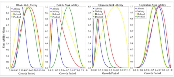
where M(A, B) is a normalization factor defined as: 275 M(A, B) = ( A−1 A+B−2) A−1×(1− A−1 A+B−2) B−1 (13)
Two organ-type-specific parameters sinkA(o) and sinkB(o) control the 276
function shape, as illustrated in the result section Fig. 4. Thus, the sink 277
activity of an organo at ranki starts from initT T(o, i) and lasts during the 278
organ’s expansion duration epdT T(o, i). 279
Second step: Total demand. The plant total demand sumSink(d) is com-280
puted as the scalar product of the number of existing organs by their sink 281 strength SAP(d, o, i): 282 sumSink(d) =X t X i SAP(d, o, i) (14)
Third step: biomass partitioning to organs. The total dry biomass CDM(d) 283
that is produced at day d is allocated to every individual organs propor-284
tionnally the ratio of their sink strength SAP(d, o, i) to the total plant de-285
mandsumSink(d). For example the biomass allocated to an individual blade 286
indM S(d, blade, i) (g.m−2) of blade rankingi is:
287
indM S(d, blade, i) = CDM(d)×SAP(d, blade, i)
sumSink(d) (15)
Total blade biomass organM S(d, blade) (g.m−2) at time d is the sum of all
288
individual blade biomass: 289
organM S(d, blade) =X
i
indM S(d, blade, i) (16)
Similarly, individual and total petiole biomass (indM S(d, petiole, i) andorganM S(d, petiole), 290
g.m−2) are simulated, as well as individual and total internode biomass
291
(indM S(d, internode, i) and organM S(d, internode), g.m−2), and
capitu-292
lum biomass(indM S(d, capitulum, i)organM S(d, capitulum), g.m−2).
2.2. Field experiments and measurements
294
Experiments and measurements for designing and constructing modules 295
which are directly inherited from SUNFLO are not presented in this paper, as 296
they are described in detail in Lecoeur et al. (2011). Data used for SUNLAB 297
parameters estimation, simulation and application include three datasets, re-298
spectively entitled as “2001”, “2002a”and “2002b”. They all come from field 299
experiments conducted in 2001 and 2002 at SupAgro experimental station at 300
Lavalette (43◦ 36’N, 3◦ 53’ E, altitude 50 m) on a sandy loam soil for four 301
genotypes “Albena”, “Heliasol”, “Melody” and “Prodisol”. In “2001”, Sun-302
flowers were sown on 5 May 2001 at a density of about 6 plants m−2 and a
303
row spacing of 0.6 m, in a randomized complete block design with four repli-304
cations. Plots measured 5.5.×13.0m. In the other two datasets, experiments 305
were conducted with the same plant arrangement. But sunflowers were sown 306
on 15 May 2002 and plots measured 8.0×8.0m. During the experiment, 307
meteorological data such as temperatures and radiation were recorded. The 308
total amount of water available for the plant was calculated as the differ-309
ence between soil water content at field capacity estimated at the beginning 310
of the experiment and soil water content at 10% of maximal stomatal con-311
ductance. The fraction of transpirable soil water (FTSW) remaining in the 312
soil at a given date was calculated as the ratio of actual plant-available soil 313
water content to the total plant-available soil water content (Lebon et al., 314
2006). Organogenesis was described based on the phenomenological stages 315
that were recorded every 2-3 days (Lecoeur et al., 2011). Once a week, six 316
plants per genotype were harvested. Individual leaf areas were estimated 317
from blade lengths and widths. All the above-ground organs (blades, peti-318
oles, stem, capitulum and seeds) were collected and then oven-dried at 80◦C 319
for 48 h. The dry weights of these organs were measured by compartments. 320
Daily radiation interception efficiency RIE(d) and daily radiation use ef-321
ficiency RU E(d) were respectively calculated and estimated based on field 322
measurements as in (Lecoeur et al., 2011). In all experiments, the crop was 323
regularly irrigated and fertilized to avoid severe water deficits and mineral 324
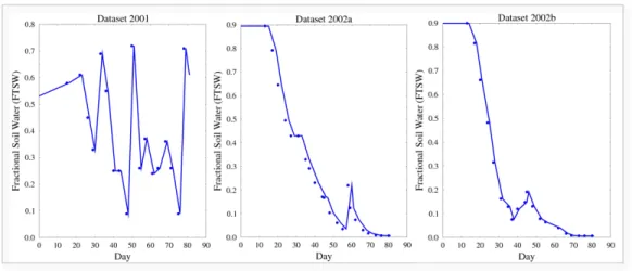
deficiency. But in practice, the three experiments showed different water 325
deficit conditions. The index F T SW of the three experiments, which can 326
represent the water stress level, is illustrated (Fig.2). Since the experiment 327
measurements were carried out every a few days, an interpolation on exper-328
imental data was drawn to make the contrast clearer. Datasets “2001” and 329
“2002a” correspond to contrasted environmental conditions and are used to 330
calibrate SUNLAB model while “2002b” is used for model evaluation. 331
[Figure 2 about here.] 332
2.3. Parameter analysis
333
Four genotypes “Albena”, “Melody”, “Heliasol” and “Prodisol” are con-334
sidered in this paper. These genotypes have been characterized by a large 335
study of genetic improvement of sunflower over the last 30 years, and they 336
are four of those most widely grown varieties in France from 1960 to 2000 337
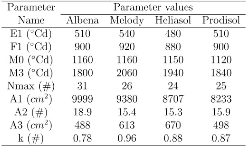
(Vear et al., 2003). SUNLAB parameters can be decomposed in two subsets. 338
One subset contains the parameters inherited from SUNFLO which keep the 339
same values in SUNLAB (Table 1). 340
[Table 1 about here.] 341
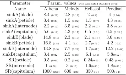
The other subset contains 17 additional parameters, that are introduced in 342
SUNLAB, as was presented in section 2.1. They include 12 parameters that 343
drive the sink competition (SR,sinkA,sinkB for four types of organs) and 5 344
parameters, that are used to adjust or define initial and final organ expansion 345
thermal times: initT T Adjust (◦C days), epdT T A (◦C days), epdT T B (◦C 346
days), internodeEpdT T (◦C days), and capitulumEpdT T (◦C days). Note 347
that the sink strength of blades SR(blade) is set to 1 as a reference value 348
(Christophe et al., 2008), therefore only 16 parameters are included in the 349
sensitivity analysis and estimation procedure. 350
The non-linear generalized least squares method with Gauss Newton al-351
gorithm for optimization (Cournede et al., 2011) was used for estimating the 352
16 parameters of four genotypes. The target field data include(i)total blade 353
mass, total petiole mass, total internode mass, and capitulum mass, all col-354
lected once a week during 15 weeks in total, and (ii) individual blade mass. 355
Regarding the target field data at organ scale used for parameter estimation, 356
only individual blade area data was available. All organs were only weighted 357
at compartment scale. In particular, independent blade mass data was not 358
available, while these data are required for a better estimation of SUNLAB 359
parameters. Therefore, profiles of individual blade mass were estimated as 360
follows: at each date when total blade mass and total blade areas were mea-361
sured at compartment level, a virtual SLAvalue was computed as the ratio 362
of these two quantities and was used to generate a set of individual blade 363
mass from the sequence of areas. The model can thus be viewed as a dynamic 364
interpolation solver that generates both blade areas and mass between those 365
fixed measurement dates. Since these measurements at individual scale were 366
performed 6 times, the estimated blade mass represent around 150 data for 367
each genotype, to be added to the 60 data at compartment scales, giving a 368
total of around 210 observation data used for the parameter estimation of 369
each genotype. 370
A sensitivity analysis was performed on SUNLAB parameters to under-371
stand their relative influence on determining the main model output, the 372
yield Y. A global method was used, the Sobol method (Saltelli et al., 2000; 373
Wu and Cournede, 2010). In this method, parameters are considered as 374
random variables that are drawn from predefined distributions, chosen here 375
as uniform distributions since no a priori knowledge is available for the 16 376
SUNLAB parameters. Plausible interval boundaries are defined: the lower 377
boundary is set as 0.5 times of the parameter’s minimum estimated value 378
among all genotypes, and the upper boundary is set as 1.5 times of the pa-379
rameter’s maximum estimated value. This allows computing an estimator 380
of the output variance, V(Y). The first-order sensitivity index of a given 381
parameter Xi can thus be defined as:
382
Si =
VXi(E∼Xi(Y|Xi)
V(Y) (17)
where the inner expectation operator is the mean ofY taken over the possible 383
values of all other parameters except Xi(E∼Xi) while keepingXi fixed. Then 384
outer variance is taken over all possible values of Xi. Similarly, higher order 385
sensitivity indices can be defined to characterize the effects of interactions 386
between parameters on the output variance. Sensitivity indices are normal-387
ized thanks to the well-known formula of variance decomposition. Here, 1000 388
parameter sets are generated from the Sobol sequence in the calculation. 389
This crop model SUNLAB and the statistical analysis methods are inte-390
grated in the platform PYGMALION (Courn`ede et al., 2013): this platform 391
is currently developed and used in the laboratory of Applied Mathematics 392
and Systems at Ecole Centrale Paris, and is available to a few other labs for 393
collaborative research projects. Programmed in C++ computer language, it 394
is dedicated to the mathematical analysis of plant growth models, including 395
the parameter estimation and sensitivity analysis methods used in this pa-396
per. It comprises approximately 20 classical and new models of plant growth, 397
among which are Greenlab (Hu et al., 2003), PILOTE (Mailhol et al., 1997, 398
2004), STICS (Brisson et al., 1998), SUNFLO (Casadebaig et al., 2011) and 399 SUNLAB. 400 3. Results 401 3.1. Sensitivity analysis 402
A sensitivity analysis was performed on the 16 parameters (described in 403
2.3) of SUNLAB for the yield, using the Sobol method of variance decompo-404
sition. Results are gathered in Table 2 for the most influential parameters. 405
The sum of all first order indices was 0.87, which means that the part of 406
variance due to parameter interactions was less than 15%: this justifies that 407
the sensitivity analysis of this model can be grounded on first-order indices 408
of parameters. The most influential parameters are those driving the dynam-409
ics of capitulum sink variations, sinkA(cap) and sinkB(cap), accounting for 410
51% and 12% respectively of the yield variance. The only other parameter 411
with significant sensibility index is a parameter of internode sink variation, 412
sinkA(intern). All other parameters account for less than 5% of the yield 413
variance. This result suggests that dynamics of biomass allocation to the 414
capitulum, more than the value of its sink, are important for yield determi-415
nation. 416
[Table 2 about here.] 417
3.2. Model parameterization
418
3.2.1. Parameter estimation for four sunflower genotypes
419
The SUNLAB parameters were estimated for the four different geno-420
types (“Albena”, “Melody”,“Heliasol”, and “Prodisol”) using experimental 421
datasets of “2001” (non-limiting conditions) and “2002a” (with water deficit). 422
The values of the 12 sink competition related parameters are shown in Table 423
3 with the associated standard deviation. 424
These parameter values were independently estimated for each genotype, 425
i.e. noa priori genotypic correlations were imposed. This allows comparing 426
the genotypes according to their parameter values. The standard error could 427
allow testing the significance of differences between two parameter values, but 428
this would only be an approximate result since the number of observations 429
that directly influence the estimation of each parameter was unknown. to 430
change with the results of the test. Qualitative observations can nevertheless 431
be done. For example, blade parameter sinkA(blade) in the sink variation 432
function of blades appears significantly different between four genotypes, 433
while no clear evidence of genotypic variability was found for capitulum sink 434
strength ratio SR(capitulum) (see also Fig. 4). The internode sink ratio, 435
SR(internode), was found different for genotypes “Albena” and “Melody”, 436
but took similar values for “Heliasol” and “Prodisol”. 437
[Table 3 about here.] 438
3.2.2. Model performances: reproducing genotype-induced variability
439
Even when grown under non-limiting controlled conditions, the four stud-440
ied varieties presented some phenotypic variability, that might be intrinsically 441
regulated by genotypic influences. This phenotypic variability was in partic-442
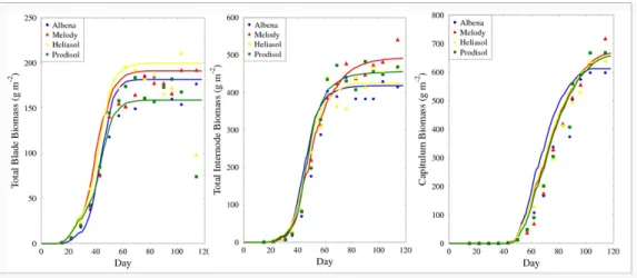
ular observed on daily radiation interception efficiency RIE(d), total blade 443
areaAA(d), leaf numberN(d), cumulated dry biomassCDM(d) and biomass 444
partitioning. This is illustrated in Fig. 3 for dry mass compartments (blade, 445
internode and capitulum) with the “2001” experimental dataset. This figure 446
also illustrates the model ability to reproduce this (presumably) gentoypic 447
variability. 448
[Figure 3 about here.] 449
The estimated parameter values (Table 3) allow tracking back the dy-450
namics of biomass allocation and analyzing the internal mechanisms under-451
lying sink competition. For instance, compared to “Prodisol”, blades of 452
“Albena” entered earlier in the competition for biomass but the capitulum 453
reached its maximum demand later (Fig. 4): this may explain that in the 454
end “Albena” had bigger total blade biomass but smaller capitulum biomass 455
than “Prodisol”(Fig. 3). Genotypic characterization can also come from the 456
biomass accumulation module: “Melody” had larger internode and capitu-457
lum biomass than “Heliasol”, and they had similar blade biomass, as can 458
be seen in Fig. 3. This was due to a higher radiation use efficiency of the 459
“Melody” genotype. 460
[Figure 4 about here.] 461
3.2.3. Model performances: reproducing environment-induced variability
462
The SUNLAB model was calibrated using “2001” and “2002a” exper-463
imental datasets that included data for plants grown without water deficit 464
(“2001”) and plants grown under water deficit (“2002a”). The parameterized 465
SUNLAB model was able to simulate the phenotypic variability induced by 466
the two contrasted environmental conditions of “2001” and “2002a” datasets. 467
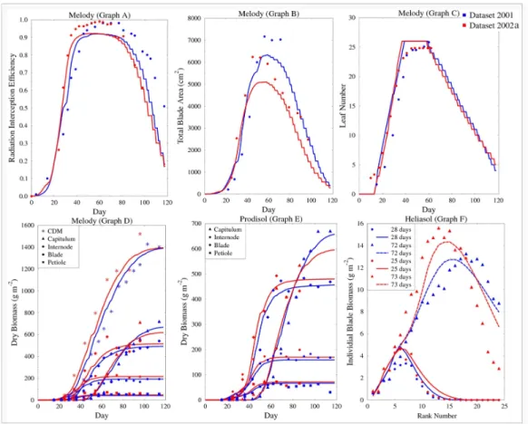
This is illustrated in Fig.5 that shows experimental data and simulations of 468
radiation interception efficiencyRIE(d), total blade areaAA(d), leaf number 469
N(d), cumulated dry above-ground biomassCDM(d) and biomass compart-470
ments (capitulum, blades, petioles, internodes) for the “Melody” genotype. 471
It can be noticed that “Melody” was not very sensitive to water stress since 472
the dry mass accumulation did not significantly vary. Graph B shows that 473
there were under-estimations of total blade area. This was due to the mod-474
eling equations of leaf area (see equation 6 and equation 7). These equations 475
are inherited from SUNFLO model and define a common formula for all geno-476
types to calculate total leaf area based on genotype-specific parameters A2 477
andA3. This common formula does not allow to account for all the genotypic 478
variance of total leaf area: possible improvements on this part of the model 479
are discussed in section 4. Graph E and Graph F of this Fig.5 present some 480
details on two other genotypes: biomass compartments of “Prodisol” and in-481
dividual blade mass profile for “Heliasol”. Water stress induced a decrease in 482
the capitulum biomass of “Prodisol” plants, despite a slight increase in blade 483
biomass. The effect of water stress can also be observed on the individual 484
blade mass profile of “Heliasol” plants: blades on the last ranks grew less in 485
water deficit conditions (“2002a”) than in standard conditions (“2001”). 486
[Figure 5 about here.] 487
3.3. Model evaluation
488
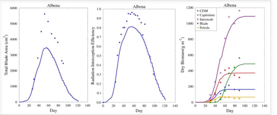
In order to test the model predictive ability, SUNLAB was confronted 489
to an additional experimental dataset “2002b”, that was not used for the 490
parameterization step. Fig. 6 presents some phenotypic traits for the “Al-491
bena” genotype: for total blade areas and radiation interception efficiency, 492
data were underestimated by model predictions, total dry biomass was also 493
proportionally affected, but the results were reasonable for the biomass com-494
partment dynamics. The root mean square error (RMSE) of organ mass 495
for genotype “Albena”, calculated on days with available experimental data, 496
was 36.4 and its coefficient of determination was 0.95. However, it has to be 497
noticed that this evaluation process was still at a preliminary step since our 498
additional experimental dataset “2002b” was measured in experimental con-499
ditions similar to those of the “2002a” dataset which was used to calibrate 500
the model. 501
[Figure 6 about here.] 502
3.4. Model Application: an exploratory study on specific leaf area
503
Specific leaf area (SLA) is an important variable in plant growth mod-504
eling. In most dynamic models, it is usually used to determine blade sur-505
face area values from blade biomass, as in GREENLAB (Christophe et al., 506
2008) or in TOMSIM (Heuvelink, 1999). Since blade area in turn determines 507
the biomass production, accurate estimation of SLA is mentioned as a ma-508
jor source of error in models and implies difficulties in obtaining a reliable 509
computation of leaf area index, which is the main component of biomass 510
production modules (Heuvelink, 1999; Marcelis et al., 1998). It is however 511
generally considered as constant, although it has been shown, for instance 512
on wheat (Rawson et al., 1987), that SLA varies according to genotypes, 513
leaf ranks and leaf growing periods. Regarding sunflower, the variations of 514
SLA and the factors influencing them are still poorly known. As SUNLAB 515
can simulate dynamics of individual blade mass profiles independently from 516
those of blade areas, the SLA can be computed as a model output, contrary 517
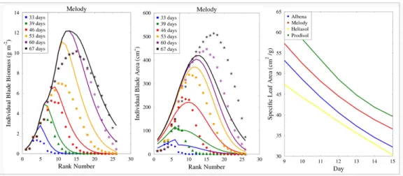
to the classical situation where it is taken as input. In Fig.7, the simulated 518
and observed values for individual blade areas and masses of “Melody” in 519
the “2001” dataset are displayed for each blade rank and six different growth 520
stages. 521
[Figure 7 about here.] 522
The SLA was computed at the time when individual blades have reached 523
their highest mass on 67th day. SLAs are illustrated for blades ranking from
524
9 to 15 which are those whose individual blade mass and area had the best 525
accordance to the field data (Fig. 7). The root mean squared error (RMSE) 526
of SLA for these blades ranking from 9 to 15 was 11 and the coefficient of 527
variation (CV) was 25%. But for all blades on 67th day, including those
528
whose individual blade leaf areas were poorly simulated, the RMSE of SLA 529
for genotype Melody became 35, with CV value 76%. The computed SLA 530
showed some variability among the four genotypes. But since the current 531
SUNLAB parameters came from reconstructed individual blade masses, these 532
simulated SLA results are expected to be improved with better experimental 533
data in the future. Moreover, the modeling of individual leaf area should be 534
improved as well for more accuracy on this result. 535
4. Discussion and conclusion
536
Models in the breeding process. After further tests and improvements, this 537
new SUNLAB model should present robust enough predictive capacities and 538
ability to differentiate between genotypes in order to be proposed as a proper 539
tool for the understanding of crop phenotypes induced by genotype × en-540
vironment interactions. Practical considerations should also be examined 541
in our context of model application, i.e. transferring model-based informa-542
tion to breeders. This kind of information could be for instance recommen-543
dations on optimal environmental conditions or management practices for 544
a given genotype; the identification of particular features (a subset of the 545
model parameters, for instance) to focus on in the breeding process in order 546
to create variants with some targeted traits; environmental characterization 547
for genotypes performances; or the prediction of crop growth and harvest. 548
SUNLAB has the potential to be used in studying the link between crop 549
model parameters and genetic information. As stated in Messina et al. 550
(2006), the breeding of higher-yielding crop plants would be greatly accel-551
erated if the phenotypic consequences of changes at some genetic markers 552
of an organism could be reliably predicted. Recently, quantitative trait loci 553
(QTL) information has been incorporated into some organ-level crop models 554
(Reymond et al., 2003; Yin et al., 2006; Xu et al., 2011). To address the 555
link between model parameters and QTL, well designed models and suit-556
able experimental data are required. Appropriate model structures allow 557
sufficient physiological feedback features to be incorporated. Model input 558
parameters should be designed to be grounded potentially in gene-level un-559
derstanding (Yin et al., 2004). It requires the plant growth model parameters 560
having biological meaning to represent genetic coefficients (Yin and Struik, 561
2010; Tardieu, 2003). The organ-level model SUNLAB and its parameters 562
are expected to meet the requirements. In line with what has been done 563
for pepper in Alimi et al. (2013), SUNLAB is considered to be used in a 564
study with an experimental database of 90 sunflower genotypes which are 565
F1 hybrid of the first filial generation resulting from a cross mating of 9 × 566
10 distinctly different parental types. After estimating SUNLAB parameters 567
for the 90 genotypes, statistical analyses of the correlations between different 568
genotypes’ parameters could reveal certain genetic links. 569
About the modeling approach: from process-based model to functional
struc-570
tural model. The design of the SUNLAB model was based on an ecophys-571
iological model, SUNFLO, that was transformed to a FSPM and enriched 572
with a mechanistic module for biomass allocation to organs. Fenni: in the
573
deleted paragraph “While there exist many excellent PBM models with
ac-574
curate model identification and growth description, it is possible to convert
575
them into FSPMs to take advantage of FSPMs’ structures and organs’
in-576
teraction, and to reduce the efforts of building a FSPM from blank. Feng
577
et al. (2010) tested using GREENLAB sink-source solver to improve the PBM
578
model PILOTE (Mailhol et al., 1997) for the crop Maize (Zea mays L.) Ac-579
tually, these previous sentences were already re-used below.. In this paper,
580
SUNLAB is a good demonstration for the crop Sunflower (Helianthus an-581
nuus L.). It defines sunflower’s structural development and it adds complex
582
biomass partitioning mechanism to SUNFLO, while it keeps certain modules
583
of this PBM model, with the advantages of inheriting its ecophysiological
584
merits...”, some sentences were actually trying to answer the first reviewer’s
question in the previous review: “ A simple conceptual representation could
586
be useful to better understand how the source-sink model (GREENLAB)
587
integrates with process-based model (SUNFLO)”. Do you think we should
588
add some more sentences as the conceptual representation of the integration
589
of FSPM module in SUNLAB?Vero: I am not sure, but I think that what 590
the reviewer meant was that we add a figure with a diagramm of the SUN-591
LAB model, don’t you think so? If so, anyway, we have not done it. In 592
process-based models (PBM), plants are usually considered only at the level 593
of organ compartments. Turning them into FSPM allows taking advantage 594
of the simulation of individual organs’ growth and of interactions between 595
organogenesis and functioning. FSPMs focuses on the development, growth 596
and function of individual cells, tissues, organs and plants in their spatial and 597
temporal contexts (Godin and Sinoquet, 2005). It is a solution to take into 598
account the plant’s architectural development and to extrapolate PBM at 599
organ level by merging the botanical knowledge on plant development with 600
the functional equations (de Reffye et al., 2008). Introducing a mechanism 601
of trophic competition at organ level in a PBM, as done in this study, opens 602
the possibility to model feedbacks effects of biomass partitioning on other 603
processes such as photosynthesis or organogenesis (Mathieu et al., 2009). 604
A more classical way to construct FSPM consists in integrating function-605
ing processes into an existing architectural model. This was done for instance 606
for trees in the AMAP- suite (Barczi et al., 2008), for grappevine in Pallas 607
et al. (2011) based on the relationships defined for organogenesis in Lebon 608
et al. (2004), or for wheat in Evers et al. (2010) who built a FSPM from 609
the ADEL-wheat model. Once plant architecture is simulated, incorporating 610
functional processes arise as a natural subsequent step in model development. 611
In particular, these 3D-mock-ups are often used to compute light intercep-612
tion. In contrast, since SUNLAB originates from a PBM, the emphasis is 613
put on modeling plant functioning, phenology and effects of water and ther-614
mal stresses, while light interception is modeled in a rather simplistic way 615
not relying on the exact 3D structure. A similar approach was applied for 616
the development of the Ecomeristem model of rice growth (Luquet et al., 617
2006) that incorporates some features (carbon supply, simulation of an ini-618
tial carbon reserve pool and the mobilisable fraction thereof) of a simple crop 619
model SARRA-H (Dingkuhn et al., 2003). Feng et al. (2010) also tested us-620
ing the GREENLAB sink-source solver to improve the PBM model PILOTE 621
(Mailhol et al., 1997) for the crop Maize (Zea mays L.). 622
Generally, our approach fits into a current general trend of development 623
of modular models, with generic modules that can be shared by other mod-624
elers. This trend goes hand in hand with the increasing number of modeling 625
platforms: Pygmalion in our case (Courn`ede et al., 2013), OpenAlea (Pradal 626
et al., 2004), GroIMP (Kniemeyer et al., 2006), etc. These platforms pro-627
vide flexible frameworks for the coupling of models or the re-use of modules 628
in different models. It reduces the efforts of building models from blank 629
and mutualizes the implementation work. SUNLAB falls within that trend 630
since most of its modules are generic and could be easily adapted to other 631
crops (e.g. biomass allocation module, biomass production module, water 632
budget,...). 633
Mechanistic modeling and empirical modeling. SUNLAB is the fruit of an ef-634
fort to make the SUNFLO model more mechanistic (through the modeling of 635
biomass partitioning). Mechanistic models generally arise from approaches 636
relating to the complex system theory: they consider the individual com-637
ponents of the system and their interactions, and what emergent properties 638
appear. They have the potential to be used out of their calibration inter-639
val, provided that the model predictive capacities have been preliminarily 640
checked. In contrast, empirical models are derived on direct descriptions of 641
observed data. They are usually regression based and provide a quantitative 642
summary of the observed relationships among a set of measured variables. 643
Most plant growth models combine in fact both modeling approaches as a 644
mixture of mechanistic modules and empirical modules. 645
It is expected that mechanistic description of ecophysiological processes 646
improves the model predictive capacities and their ability to differentiate be-647
tween genotypes (Allen et al., 2005; Minchin and Lacointe, 2005; Bertheloot 648
et al., 2011). However, the extent to which more mechanistic models are 649
necessarily better should be questioned. In particular, since the parameters 650
in mechanistic modules are assumed to have assigned biological meanings 651
and to represent properties of real system components, the reliability of the 652
underlying assumptions need to be carefully validated. I kept this sentence, 653
but I am not sure of what you meant, Fenni. Could you explain me? Fenni:
654
because the mechanistic models normally try to simulate the biological
hy-655
pothesis, the parameters in mechanistic modules have assigned biological
656
meanings. Therefore, it need more scrutiny to determine whether the
hy-657
pothesis and the biological meanings are true. I got this sentence from this
658
article: Biomedical Applications of Computer Modeling, Chapter 7.2
Em-659
pirical or mechanisticvro: ok. Do you agree with the way I modified the 660
previous sentence, then?. Thus, the appropriateness of mechanistic models 661
needs close scrutiny (Christopoulos and Michael, 2000). Moreover, the pa-662
rameterization effort of these more and more complex models should always 663
be taken into account when improving their mechanistic description, to pre-664
vent from a high level of uncertainty in the parameters which may hinder the 665
original purposes of the model in terms of prediction and genotypic differen-666
tiation. So, as stated in the introduction, a delicate trade-off has to be found 667
between mechanistic aspects and complexity, in order to provide proper tools 668
that might be used in the breeding context. 669
Parameter estimation issue: direct measurements and model inversion. Two 670
kinds of methods were involved for SUNLAB parameterization: estima-671
tion through direct measurements and estimation through statistical meth-672
ods, sometimes referenced as model inversion methods. Direct measurement 673
method enables direct access to the desired parameter via experimental mea-674
surements (Jeuffroy et al., 2006). The model inversion method, involving 675
mathematical and statistical calculations, estimates one or more parame-676
ters by confronting observed data to simulation results (Guo et al., 2006; 677
Cournede et al., 2011). 678
Direct measurement is used to estimate parameters that have biological 679
meanings, and that can be directly observable or easily calculated from mea-680
sured indicators. Parameters with biological meanings consist of two types: 681
“genotypic parameters” which differ between varieties and “crop parameters” 682
which are parameters with small variance among all genotypes. Theoretically, 683
direct measurement method is the best for estimating genotypic parameters 684
and consequently for genotype characterization. The breeder could measure 685
it directly on lines under development in experiments in order to predict the 686
expected effects (Reymond, 2001). Similarly crop parameters can be mea-687
sured directly from field data. Because of the direct and accurate measures on 688
elementary processes, these estimated parameters have advantages in terms 689
of ecophysiological relevance, parameter accuracy and genotype characteriza-690
tion, compared with model inversion method. This perspective has led to au-691
tomated and high-throughput advanced plant phenotyping (see for example 692
Granier et al. (2005), Sotirios and Christos (2009)). However, the accurate 693
elementary processes do not necessarily imply that the combination of these 694
processes will provide the same accuracy at plant scale. The nonlinear in-695
teractions between processes as well as the necessary simplifications in terms 696
of the number of ecophysiological processes considered in the model make 697
the whole plant model not a simple combination of the elementary models 698
that were well calibrated by experiments: plants are complex systems whose 699
description of elementary process interactions, plasticity and robustness re-700
mains an open issue (Yin and Struik, 2010). Therefore, parameterization 701
methods relying on model inversion to estimate parameters from experimen-702
tal data at organ or whole plant levels offers an alternative. This method can 703
ensure an optimized fitting error on training data, but the prediction error 704
on validation data has to be carefully checked to avoid over-fitting problems. 705
The parameters thus obtained have the risk to be less relevant for their bio-706
logical meanings than direct measurement, because these parameters values 707
may be altered by the error compensation from fitting whole plant processes 708
and from other simultaneously estimated parameters (Jeuffroy et al., 2006). 709
They nevertheless characterize the plant global behavior and may still be 710
used to differentiate between genotypes (Letort, 2008). 711
When parameter estimation is demanded for a high number of genotypes, 712
direct measurement method becomes impractical, because this method often 713
requires specific trials and measurements, which are complicated, costly and 714
even impossible to implement sometimes (Reymond, 2001). Routine mea-715
surement of these parameters for a large number of varieties may also pose 716
a problem, particularly when measurements require special equipment and 717
controlled condition experiments (Jeuffroy et al., 2006). Model inversion 718
method is adopted for these cases because it is experimentally less costly 719
and less time-consuming. For instance in most dynamic models, the direct 720
measurement method would often require frequent measurement points (e.g. 721
daily), while with the indirect method, data can be collected only at some 722
given time points and still allow the modellers to retrieve the past growth of 723
the crop. Parameters can even be estimated from very limited sets of data 724
(Kang et al., 2011). 725
Moreover, some parameters are “hidden”,i.e. cannot be experimentally 726
measured and can only be estimated by model inversion method. They usu-727
ally appear in mechanistic modules, because their underlying mechanisms 728
can produce emergent properties that can be difficult to disentangle a
pos-729
teriori from the resulting phenotype. It also implies that, because of their 730
interactions, these kinds of parameters cannot be obtained independently 731
from each other: the whole estimation process needs to be performed on all 732
the data at the same time (it is not possible to optimize sequentially on data 733
for different types of organs, for instance). 734
In SUNLAB, the parameters inherited from SUNFLO have biological 735
meaning and had been measured for 20 genotypes. Meanwhile, the param-736
eters involved in the new biomass allocation module are hidden parameters 737
that can only be estimated by model inversion, because the biomass alloca-738
tion process at organ level is difficult to observe and to be directly measured. 739
Limitations and perspectives
740
Modeling. From the model performances results, we can see that the mod-741
eling of blade area needs to be uppermost improved in SUNLAB. A first 742
improvement could consist in replacing the use of the logistic function by a 743
fully mechanistic approach including modeling the SLA instead of deriving it 744
a posteriori from the simulated mass and areas. Thereby, feedbacks effects of 745
trophic competition on leaf area expansion could be explored and modeled. 746
The biomass accumulation module was directly inherited from SUNFLO 747
that has been tested in different environmental conditions for 26 genotypes 748
(Casadebaig et al., 2011; Lecoeur et al., 2011) and is in line with what is classi-749
cally done in models of the same class as SUNLAB (e.g. Tomsim (Heuvelink, 750
1999), Ecomeristem (Luquet et al., 2006)). A more detailed approach, at 751
individual leaf level, could be considered by computing the amount of inter-752
cepted radiations: several methods are available (e.g. Nested Radiosity light 753
model in Evers et al. (2010) or a Monte-Carlo radiation model in Xu et al. 754
(2011)) but they require an accurate modeling of the plant structure which is 755
currently not available and would necessitate additional experimental work 756
to be parameterized. It has to be noted that SUNLAB is not stricto-sensu a 757
FSPM since no 3D shape is simulated. 758
As regards the biomass distribution module that was introduced in our 759
study, our approach is based on the concept of common pool of assimilates 760
and relative sink competition. However, some other models (e.g. ECOPHYS 761
[Lacointe et al., 2002])) and experimental observations (Pallas et al. (2008)) 762
suggest that the distance from source to sink could have an influence. An al-763
ternative approach is thus to consider transport-resistance methods, as done 764
for instance in the L-PEACH model [Allen et al., 2005]: although these meth-765
ods are biologically more relevant, they are generally complex and the result-766
ing biomass distribution remains highly dependent on the determination of 767
sink activity. Bancal and Soltani [2002] compared the partitioning coeff-768
cients obtained from an improved version of the transport-resistance model 769
of [Minchin et al., 1993] to the classical sink-based partitioning model: they 770
concluded that the resistance to flux propagation has an influence only in 771
pathologic cases of very low source activity and that resistance terms could 772
be abandoned in most cases as they are only a mathematical burden whose 773
parameter values are very diffcult to measure experimentally. In our source-774
sink approach, the main limiting factor is not the geometrical distance but 775
the topological organization of source and sinks (i.e. the number of other 776
sinks in a source-sink pathway) (Letort, 2008). 777
what do you mean exactly, with this solution?Fenni: I mean the feedback
778
effects of trophic competition on other plant functions could be simulated
779
in the future. It was written in the paragraph you deleted as such
“How-780
ever, the lack of trophic competition simulation may hinder the simulation of
781
feedback effects of biomass partitioning on other processes. As Pallas et al.
782
(2008) state, trophic competition influenced the organogenesis of grapevine
783
in their research. They suggest that a modeling approach simulating sink
784
strength variation and the local effects of sink proximity would be more
vant than a model considering only development as a function of thermal time
786
or the global distribution of available biomass”. I tried to write the modeling
787
limitations in term of blade area modeling, and the modeling of feedback
ef-788
fects of trophic competition. Besides, the third reviewer asked in last review
789
“why the biomass accumulation is a very global level compared to the organ
790
level elsewhere. How do you justify these differences?” I answered him that
791
“The biomass accumulation module is directly inherited from SUNFLO while
792
the biomass distribution module is completely changed, as the first step of
793
adapting it into a FSPM model. Its performance and evaluation have shown
794
satisfactory results. Next step will be to add feedback effects of biomass
795
partitioning to the model, which will improve the simulation of
morphogen-796
esis, biomass production etc. This point is discussed in the Discussion and
797
conclusion session in this new version of paper”. Therefore I discussed here
798
why feedback effects need to be simulated. This is also my answer to the
799
first reviewer’s question “where is the biomass production’s under-estimation
800
from” and “why the upper leaves’ SLA can not be well simulated”. I put
801
the reasons to the bad simulation of blade area, especially the upper leaves’
802
blade area. I mentioned some improvements of biomass production modeling
803
can be planned in the future, such as the feedback effects of biomass
distribu-804
tion on blade area modeling, and also the consequent simulation of biomass
805
production. I also mentioned that to improve the simulation of SLA,
“Be-806
sides the approach that the logistic function, which is used to model leaf area
807
in SUNLAB, can be compared with other functions, the feedback effect of
808
trophic competition on leaf area expansion can be investigated and modeled.”
809
So to sum up, with the limitation of blade area modeling, I tried to answer
reviewers’ three questions: 1, why the biomass production is a very global
811
level compared with biomass distribution; 2, where is the under-estimation
812
of biomass production from; 3, why did we state that the SLA simulation of
813
upper leaves are not well simulated. 814
Fenni: the deleted sentences of leaf senescence “In SUNLAB, leaf
senes-815
cence is modeled to occur between phenology stages M0 and M3. The
816
phenology timing “CTT(d)” is affected by water stress, which affects
con-817
sequently the rate of leaf senescence. Its leaf senescence start time can be
818
better modeled, since sunflower leaves senescence may occur beforeM0 stage
819
in drought stressed conditions”, is actually an answer to the second reviwer’s
820
question in previous review: “Leaf senescence is in the model expected to
821
occur between the stages M0 and M3. In the SUNLAB model, the impact
822
of the drought stress on the phenology is tsaken into account (page 6-line 54
823
to page 7-line 20); however this point should benefit to be discussed, as
sun-824
flower leaves senescence may occur before the M0 stage in drought stressed
825
conditions”. I tried to mention the limit of leaf senescence modeling. Sunlab
826
doesn’t simulate leaf senescence in strong stress, occuring before M0. Ok, 827
I put some back, then. Do you agree? Besides, leaf senescence is currently 828
affected by water stress only (through the phenology timing “CTT(d)” that 829
affects consequently the rate of leaf senescence) and occurs between phenol-830
ogy stages M0 and M3 while, in reality, it may occur before M0 stage in 831
severe drought conditions. Therefore, the SUNLAB leaf senescence may need 832
also modifications and could include the effects of other environmental cues 833
such as day length and temperature, and various biotic and abiotic sources of 834
stress, that can affect the initiation and progress of leaf senescence (Aguera 835