TECHNICAL SCIENCES, Vol. 63, No. 3, 2015 DOI: 10.1515/bpasts-2015-0089
Recent developments in simulation-driven multi-objective design
of antennas
S. KOZIEL
1∗and A. BEKASIEWICZ
21
Engineering Optimization & Modeling Center, School of Science and Engineering, Reykjav´ık University, Menntavegur 1, 101 Reykjav´ık, Iceland
2
Faculty of Electronics, Telecommunications and Informatics, Gdansk University of Technology, 11/12 Narutowicza St., 80-233 Gdansk, Poland
Abstract.This paper addresses computationally feasible multi-objective optimization of antenna structures. We review two recent techniques that utilize the multi-objective evolutionary algorithm (MOEA) working with fast antenna replacement models (surrogates) constructed as Kriging interpolation of coarse-discretization electromagnetic (EM) simulation data. The initial set of Pareto-optimal designs is subsequently refined to elevate it to the high-fidelity EM simulation accuracy. In the first method, this is realized point-by-point through appropriate response correction techniques. In the second method, sparsely sampled high-fidelity simulation data is blended into the surrogate model using Co-kriging. Both methods are illustrated using two design examples: an ultra-wideband (UWB) monocone antenna and a planar Yagi-Uda antenna. Advantages and disadvantages of the methods are also discussed.
Key words:computer-aided design (CAD), antenna design, multi-objective optimization, surrogate models, evolutionary algorithms.
1. Introduction
One of the most important steps in the design process of antenna structures is adjustment of their geometry and/or ma-terial parameters. The aim is to satisfy given performance specifications concerning antenna reflection, gain, radiation pattern, and, more and more often, physical dimension (size, footprint) [1–39]. For the sake of reliability, the adjustment process normally relies on high-fidelity electromagnetic (EM) simulation [1–3]. It is particularly important for contemporary structures for which theoretical models either are not available or are very inaccurate. Also, in many cases it is necessary to account for EM interactions between the antenna itself and its environment (connectors, housing, installation fixtures, etc.).
Perhaps the most common approach to geometry adjust-ment is parameter sweeps guided by engineering insight. Un-fortunately, this method is laborious and does not guaran-tee optimum results, especially when the number of indepen-dent parameters is large. Automated geometry optimization is therefore highly desirable, however, quite challenging [37–39]. Majority of conventional techniques (such as gradient-based algorithms or derivative free methods, e.g., pattern search al-gorithms) require considerable number of objective function evaluations (and, associated EM simulations) to yield an op-timized design [4]. Recent availability of adjoint sensitivi-ty techniques [5, 6] through certain commercial simulation software packages (e.g., [7, 8]) revived interest in gradient optimization. On the other hand, surrogate-based optimiza-tion (SBO) techniques [9–13] allow for dramatic reducoptimiza-tion of the design optimization costs by shifting most of the opera-tions into cheap replacement models (surrogates). The latter,
in case of antennas, are normally constructed using coarse-discretization EM simulations [14].
For the sake of simplicity, most of antenna optimization problems are reformulated as single objective ones, where one primary objective is handled directly, whereas the others are controlled through appropriately defined constraints or penal-ty functions ([15]). However, real-world antenna design tasks are multi-objective ones. In particular, if the designer pri-orities are not clearly defined beforehand, identifying a set of alternative design representing the best possible trade-offs between conflicting objectives may be of fundamental im-portance (e.g., in order to determine limitations of a given antenna structure and its suitability for a given application) [16–19]. Nowadays, population-based metaheuristics are un-doubtedly the most popular solution approaches for handling multi-objective antenna design problems. Techniques such as multi-objective genetic algorithms (GAs) and particle swarm optimizers (PSO), e.g., [16, 18–23], allow finding the entire Pareto front in one algorithm run. However, their disadvan-tage is high computational cost (hundreds, thousands or even tens of thousands of objective function evaluations), which becomes a serious bottleneck if high-fidelity discrete EM sim-ulations are involved in antenna evaluation process.
Recently, two computationally efficient techniques for multi-objective design optimization of antennas have been proposed [24, 25]. Both methods rely on fast response sur-face approximation (RSA) surrogates created from sampled coarse-discretization EM simulation data, as well as refine-ment procedures intended to obtain representations of the Pareto-optimal sets at the high-fidelity EM antenna model lev-el. The refinement strategy adopted in [24] is point-by-point
identification using designs sampled from the initial Pareto set (obtained by optimizing the RSA) model, and suitable re-sponse correction techniques. In [25] refinement is realized by blending sparsely sampled high-fidelity EM model data into the RSA surrogate using Co-kriging [26]. In this paper, we review both methods, provide their unified formulation, il-lustrate and compare them using examples (an ultra-wideband monocone, and a planar Yagi-Uda antenna), as well as discuss their advantages and disadvantages.
2. Multi-objective antenna design using RSA
models and variable-fidelity EM simulations
In this section, we formulate the multi-objective antenna design problem and introduce variable-fidelity EM models. We also describe Kriging and Co-kriging interpolation as fundamental tools for creating response surface approxima-tion (RSA) surrogates utilized throughout the optimizaapproxima-tion process. Finally, we describe the optimization flow including two alternative options for Pareto set refinement.
2.1. Multi-objective antenna design. problem formulation. LetRf(x)be a response (e.g., reflection or gain versus
fre-quency) of an accurate model of the antenna structure under design. The responseRf(x) is obtained using high-fidelity
EM simulation. Here,xis a vector of designable parameters, i.e., antenna dimensions.
We consider Nobj design objectives, Fk(x), k = 1, . . .,
Nobj. A typical performance objective would be to minimize antenna reflection over a certain frequency band of interest, and to ensure that |S11| < −10 dB over that band. There
might be also geometrical objectives such as to minimize
Fk(x) = A(x) – the antenna size defined in a convenient way (e.g., maximal lateral size, height, the maximal dimen-sion, area of the footprint, antenna volume). Similar objectives can be formulated with respect to antenna gain, radiation pat-tern, efficiency, etc.
IfNobj >1then any two designsx(1)andx(2)for which
Fk(x(1)) < Fk(x(2)) and Fl(x(2)) < Fl(x(1)) for at least one pair k 6= l, are not commensurable, i.e., none is better than the other in the multi-objective sense. We define Pareto dominance relation≺[27] saying that for the two designsx
andy, we havex≺y(xdominatesy) ifFk(x)< Fk(y)for allk= 1, . . ., Nobj. The goal of the multi-objective optimiza-tion if to find a representaoptimiza-tion of a so-called Pareto front (of Pareto-optimal set)XP of the design spaceX, such that for anyx∈XP, there is noy∈X for whichy≺x[27]. 2.2. Variable-fidelity electromagnetic models. As men-tioned in the introduction, the high-fidelity modelRf is
com-putationally too expensive to be handled directly in multi-objective optimization. In this work, we speed up the design process by utilizing an auxiliary low-fidelity modelRc, which
is a coarse-discretization counterpart ofRf. By appropriate
mesh density manipulation and possible other simplifications (see, e.g., [28]),Rc can be made 20 to 50 times faster than
Rf, however, at the expense of some accuracy degradation.
Because of this, as well as the fact that direct multi-objective optimization is usually too expensive even at theRclevel, our
optimization methodology exploits response surface approxi-mation models briefly described in the following Subsec. 2.3 and 2.4. The optimization algorithm is formulated in Sub-sec. 2.5.
2.3. Surrogate modeling. Kriging interpolation. Response surface approximation surrogates play a key role in the op-timization methodology described in Subsec. 2.5. The first part of the process (identification of the initial Pareto set) is realized using a Kriging interpolation model constructed from sampled coarse-discretization model data. Kriging is a popular technique to interpolate deterministic noise-free data [29]. LetXB.KR={x1KR, x2KR, . . ., xN KRKR } ⊂XRbe the base (training) set andRc(XB.KR)the associated low-fidelity
model responses. The Kriging interpolant is derived as
Rs.KR(x) =M α+r(x)·Ψ−1·(Rf(XB.KR)−F α), (1)
where M and F are Vandermonde matrices of the test point x and the base set XB.KR, respectively. The coeffi-cient vector α is determined by Generalized Least Squares (GLS). r(x) is an 1×NKR vector of correlations between the point x and the base set XB.KR, where the entries are
ri(x) = ψ(x,xiKR), and Ψ is a NKR×NKR correlation matrix, with the entries given by Ψi,j =ψ(xiKR, x
j KR). In
this work, the exponential correlation function is used, i.e.,
ψ(x,x′) = exp(P
k=1,...,n−θk|xk −x′k|), where the
para-meters θ1, ..., θn are identified by Maximum Likelihood
Es-timation (MLE). The regression function is chosen constant,
F = [1...1]T andM = (1).
2.4. Surrogate modeling. Co-kriging. One of the Pareto set refinement strategies, considered in this work, relies on com-bining information from EM simulations of various fidelities. Here, it is realized using Co-kriging [30]. Co-kriging is an ex-tension of Kriging, which allows blending the low- and high-fidelity EM simulation data into one surrogate by exploiting correlations between the models of various fidelities [29].
Generation of a Co-kriging model is carried out through sequential construction of the two Kriging models: the first modelRs.KRc composed from the low-fidelity training
sam-ples (XB.KRc,Rc(XB.KRc)), and the secondRs.KRd
mod-el generated on the residuals of the high- and low-fidmod-elity samples (XB.KRf, Rd), where Rd = Rf(XB.KRf)−ρ·
Rc(XB.KRf). The parameterρis a part of MLE of the
sec-ond model. In the absence of Rc(XB.KRf), they can be
approximated by the first model, i.e., as Rc(XB.KRf) ≈
Rs.KRc(XB.KRf). Configuration (the choice of the
correla-tion funccorrela-tion, regression funccorrela-tion, etc.) of both models can be adjusted separately for the low-fidelity dataRc and the
resid-uals Rd, respectively. Moreover, both models use the
expo-nential correlation function together with constant regression functionF= [1 1. . . 1]T andM = (1).
The final Co-kriging modelRs.CO(x)is defined similarly
as in (1), i.e.,
where the block matricesM, F, r(x) and Ψ of (6) can be written as a function of the two underlying Kriging models Rs.KRc andRs.KRd: r(x) = [ρ·σ2 c·rc(x), ρ2·σ2c·rc(x, XB.KRf) +σ 2 d·rd(x)], Ψ = " σ2 cΨc ρ·σ2c·Ψc(XB.KRc, XB.KRf) 0 ρ2·σ2 c·Ψc(XB.KRf, XB.KRf) +σ 2 d·Ψd # , F = " Fc 0 ρ·Fd Fd # , M = [ρ·Mc Md], (3)
where (Fc,σc,Ψc,Mc)and (Fd,σd,Ψd,Md)of (3) are
ma-trices obtained from the Rs.KRc and Rs.KRd, respectively.
Generally,σ2
c andσd2are process variances, whileΨc(·,·)and
Ψd(·,·)stand for correlation matrices of two datasets with the
optimizedθk parameters and correlation function ofRs.KRc
andRs.KRd, respectively.
Figure 1 shows the operation of the Co-kriging model us-ing a simple analytical function example. Densely sampled low-fidelity model data supplemented with a few samples of the high-fidelity model allows achieving very good accuracy when the two types of data are blended together (Co-kriging), whereas the accuracy of the Kriging interpolation model sole-ly based on the high-fidelity data is quite limited.
Fig. 1. Co-kriging modeling concept [25]: high-fidelity model (—), low-fidelity model (- - -), high-fidelity model samples (), low-fidelity model samples (◦). Kriging interpolation of the high-fidelity model samples (-·-) is not an adequate representation of the high-fidelity model (due to the limited data set size). Co-kriging interpo-lation (· · · ·) of blended low- and high-fidelity model data provides
much better accuracy at low computational cost
2.5. Optimization algorithm: obtaining initial Pareto set. The initial approximation of the Pareto set is obtained by multi-objective optimization of the fast surrogate model con-structed using Kriging interpolation (cf. Subsec. 2.2) and based on sampled low-fidelity EM model data. The design of experiments approach utilized here is Latin Hypercube Sam-pling [31]. The Kriging modelRs.KR is very fast, smooth,
and, consequently, easy to optimize. In some cases it might be necessary to perform initial reduction of the design space, that is, identify the subset of the design space containing the Pare-to front (which is normally a small part of the original design space [32]). This step is necessary for highly-dimensional de-sign spaces where, without dede-sign space reduction, the num-ber of training samples necessary to ensure sufficient
surro-gate model accuracy is impractically large. Interested reader is referred to [32–34] for exposition of simple design space reduction methods.
Having constructed Rs.KR, we apply a multi-objective
evolutionary algorithm (MOEA) to find a set of designs rep-resenting Pareto-optimal solutions with respect to the objec-tivesFk of interest. Here, we use a standard multi-objective evolutionary algorithm with fitness sharing, Pareto-dominance tournament selection, and mating restrictions [27].
The design optimization flow leading to identification of the initial Pareto set representation is the following:
1. (Optional) Perform design space reduction 2. Sample the design space and acquire theRc data;
3. Construct the Kriging interpolation modelRs.KR;
4. (Optional) Correct the Kriging modelRs.KR using space
mapping;
5. Obtain the Pareto front by optimizingRs.KRusing MOEA;
Note that the high-fidelity modelRf is not evaluated in
the above procedure. The two method of refining the initial Pareto set so that it can be elevated to the high-fidelity model level are described in Subsecs. 2.6 and 2.7. Step 3 can be executed in case of considerable discrepancy betweenRs.KR
andRf. In that case, before finding the Pareto set, the Kriging
model is enhanced by aligning it with the high-fidelity model at certain (usually small) number of designs using space map-ping. Typically, output space mapping and frequency scaling are preferred [35].
2.6. Pareto set refinement using response correction. The first refinement approach relies on point-by-point construction of the high-fidelity model Pareto set representation, starting from the designs sampled on the initial Pareto set obtained using the algorithm of Subsec. 2.5. The latter consists of the Pareto optimal solutions of the surrogate, which, because of the discrepancies betweenRc andRf, have to be corrected to adequately represent the high-fidelity model.
Let x(sk),k = 1, . . ., K, be the selected elements of the
Pareto front found by the MOEA. For simplicity of the nota-tion, the design refinement stage below is defined assuming two objectivesF1 andF2; however, it can be generalized for
any value of Nobj. The refinement stage exploits the output space mapping (OSM) [35] process of the following form:
x(fk.i+1)= arg min x, F2(x)≤F2(x(k.i)s ) F1 ·Rs(x) + [Rf(xs(k.i))−Rs(x(sk.i))] . (4)
The optimization process (4) is constrained not to in-crease the second objective as compared to x(sk). The
surro-gate modelRsis corrected using the OSM termRf(x(sk.i))−
Rs(x(sk.i)) (here, x(fk.0) = x
(k)
s ), so that the corrected
sur-rogate model coincides with Rf at the beginning of each
iteration. In practice, two or three iterations of (4) are suffi-cient to find a refined high-fidelity model designx(fk). After completing this stage, we create a set of Pareto-optimal
high-fidelity model designs. This set is the final outcome of our multi-objective optimization process.
2.7. Pareto set refinement using Co-kriging surrogates. An alternative approach to Pareto set refinement is by us-ing Co-krigus-ing surrogates (cf. Subsec. 2.4). In this case, the high-fidelity model evaluated at the designs sampled from the initial Pareto set obtained by optimizingRs.KR are included
into the surrogate model so that it becomes more and more accurate representation ofRf at least in the vicinity of the
Pareto front.
The design algorithm flow is as follows:
1. Evaluate high-fidelity modelRf at selected locations along
the current Pareto front representation;
2. Update the Co-kriging surrogateRs.CO(cf. (2));
3. Update Pareto set by optimizingRs.COusing MOEA;
4. If termination condition is not satisfied go to 2; else END When executing Step 1 for the first time, the current Pareto front representation is a Pareto set obtained using the algo-rithm of Subsec. 2.5. Typically, about 10 high-fidelity model evaluations are used in Step 1, and the number of iterations necessary to converge is two to three. Our convergence cri-terion is the maximum distance between the Pareto front es-timated in 3 and the sampledRf data (here, we use 0.5 dB
for reflection objective). It should be emphasized that – upon convergence – the entire Pareto set generated by the above procedure (not just a set of design sampled from it) is a reli-able representation of the high-fidelity Pareto set.
3. Case study 1: UWB monocone
In this section we demonstrate the multi-objective opti-mization procedure exploiting both Pareto front refinement schemes described in Subsecs. 2.6 and 2.7, respectively. The methods are illustrated using an ultra-wideband (UWB) an-tenna in the form of a monocone. The design objectives are footprint reduction and minimization of reflection.
3.1. UWB monocone – antenna description. Consider a monocone structure [24] that operates in the UWB frequency band. The antenna is fed directly through 50-Ohm coaxial line with Teflon filling and outer diameter of 0.635 mm. A para-meter vector:x= [z1z2r1]T represents antenna design
vari-ables. All parameter values are expressed in mm. The antenna geometry is shown in Fig. 2.
a) b)
Fig. 2. UWB monocone: a) 3D view; b) the cut view, after Ref. 24
Two computational models of the antenna are implement-ed in CST Microwave Studio and evaluatimplement-ed using its transient solver [7]. The high-fidelity model Rf is consists of about
1,400,000 hexahedral mesh cells and its average evaluation time is 23 min, whereas its less accurate counterpart Rc is
generated using 33,000 hexahedral mesh cells. An average simulation time of the latter is 33 s and it is 42 times faster thanRf.
In this example, we consider two design objectives: (i) minimization of antenna reflection within UWB (3.1 GHz to 10.6 GHz) frequency band (objectiveF1), and (ii)
reduc-tion of antenna footprint (objectiveF2), which is defined as
a maximum dimension out of vertical and lateral ones:S = max{2r2, z1+z2+r2}. The symbolr2= (r21−(z1+z2)2)1/2
denotes the radius of the hemisphere terminating the mono-pole.
3.2. UWB monocone. Generation of initial Pareto set. The solution space for multi-objective antenna optimization is de-fined by the lower and upper bounds l = [0 2 4]T and
u= [4 15 20]T. A Kriging surrogate model constructed using
600 low-fidelity model samples is optimized using methodol-ogy of Subsec. 2.5. The initial Pareto optimal set is shown in Fig. 3a, whereas visualization of Pareto optimal design vari-ables within a defined solution space is illustrated in Fig. 3b.
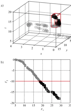
a)
b)
Fig. 3. UWB monocone antenna: a) visualization of the Pareto op-timal set (◦) in 3-dimensional solution space. The portion of the design space that contains the part of the Pareto set we are inter-ested in (red cuboid, whereF1 ≤ −10), b) the part of the Pareto
set that is of interest from the point of view of adequate antenna operation () versus the entire one mapped to the feature space (◦)
One should note that despite the Pareto set range for ob-jectiveF1being from below – 20 up to near 0 dB, the antenna
is considered as operating properly if it can provide in-band reflection below the level of−10 dB or lower. Therefore, only the designs that fulfill this requirement are considered rele-vant, and they are the subject of Pareto set refinement (cf. Subsec. 3.3 and Subsec. 3.4).
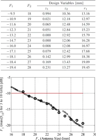
3.3. UWB monocone. Pareto set refinement using response correction. A set of 10 designs selected from the initial Pare-to set have been refined using the response correction tech-nique of Subsec. 2.6 in order to obtain high-fidelity represen-tation of the Pareto front. Two refinement steps (per design) were required to obtain the final solutions. The geometrical details of the refined solutions are listed in Table 1. A compar-ison of a Pareto front obtained throughRsmodel optimization
and its representation based on a set of 10 refinedRf model
samples is shown in Fig. 4. Table 1
Refined designs of the optimized UWB monocone antenna
F1 F2 Design Variables [mm] z1 z2 r1 −9.5 18 0.994 10.36 13.16 −10.9 19 0.021 12.18 12.97 −11.6 20 0.065 12.48 14.59 −12.3 21 0.051 12.84 15.23 −13.2 22 0.000 12.92 15.79 −14.7 23 0.000 12.06 16.28 −16.0 24 0.008 12.08 16.97 −17.1 25 0.079 12.42 17.68 −18.1 26 0.142 12.99 18.38 −18.4 27 0.169 13.43 19.09 −19.4 28 0.231 13.27 19.45
Fig. 4. Comparison of the Pareto front obtained from optimizedRs
model (◦)and eleven (see Table 1) refinedRf model designs ()
The smallest footprint of an antenna that still satisfies the minimum requirements upon its reflection (objectiveF2) is
19 mm, whereas the lowest in-band reflection (objectiveF1)
is−19.4 dB. Variations of objectives for extreme designs are 32% and 44% for the former and the latter, respectively.
The total cost of design optimization corresponds to on-ly 44 Rf model evaluations (about 17 hours of CPU time)
and it includes: 600Rcsimulations (∼14Rf evaluations) for
design of experiment (cf. Subsec. 3.2), and 10Rf for initial
evaluation and refinement (2×10 Rf) of selected samples.
The computational cost of MOEA optimization (a few dozen thousands ofRsmodel evaluations) is negligible in
compari-son with the cost of antenna models simulation, thus it is not included here.
3.4. UWB monocone. Pareto set refinement using co-kriging. A set of 10 design samples is chosen from the initial Pareto set (cf. Subsec. 2.5) and evaluated to obtain their high-fidelity model responses. Subsequently a Co-kriging method-ology of Subsec. 2.7 is utilized to refine the Pareto set. The final Pareto set representation was obtained in three iterations of the algorithm (cf. Subsec. 2.7). It should be noted that high-fidelity model samples gathered across iterations are in-corporated into the Co-kriging model to increase its accu-racy. A comparison of initial and refined Pareto set as well as 10 responses of evenly chosen high-fidelity model designs evaluated for verification purpose is shown in Fig. 5. The dimensions of selected antennas are shown in Table 2. The minimum antenna footprint that satisfies requirements upon reflection (objectiveF1)is 32% smaller in comparison to the
structure with the best in-band reflection (objective F2) of
−19.4 dB.
Fig. 5. UWB monocone antenna: initial Pareto set approximation (◦), final Pareto set obtained after three iterations of the proposed methodology (), selected high-fidelity model designs () evaluated
for verification purpose
Table 2
Selected designs of the optimized UWB monocone antenna
F1 F2 Design Variables [mm] z1 z2 r1 −10.1 18 0.23 11.79 13.61 −10.6 19 0.18 11.80 13.81 −11.1 20 0.28 11.63 14.44 −12.2 21 0.06 12.22 15.03 −13.6 22 0.06 11.76 15.81 −14.9 23 0.06 12.62 16.67 −16.5 24 0.05 12.66 17.31 −17.3 26 0.17 13.39 18.41 −17.6 27 0.21 13.38 18.98 −19.0 28 0.25 13.55 19.59
The total aggregated cost of the design optimization process corresponds to about 44 evaluations of the high-fidelity model, i.e.,∼17 hours of CPU time (including 600×
Rc≈14×Rf for initial Kriging model construction, and 3 ×10 ×Rf = 30×Rf for three iterations of the surrogate
enhancement). The computational cost of MOEA optimiza-tion of the Co-kriging model is not included for the same reasons as mentioned in Subsec. 3.4.
4. Case study 2. Planar Yagi-Uda antenna
Our second example is a planar Yagi-Uda antenna with a sin-gle director. Similarly as for the previous example, we demon-strate the use of the two design refinement demon-strategies. Here, the objectives of interest are the average gain and in-band reflection.
4.1. Planar Yagi-Uda. Antenna description. Consider a planar Yagi-Uda antenna [36] shown in Fig. 6. It is com-posed of a driven element fed by a microstrip-to-cps tran-sition, a director, and a balun. The input impedance is 50-Ohm and the structure is designated to operate on a Rogers RT6010 dielectric substrate (εr = 10.2, tanδ = 0.0023,
h = 0.635 mm). A structure is described by a eight ad-justable parameters: x = [s1 s2 v1 v2 u1 u2 u3 u4]T.
Ad-ditional parameters, i.e., Parameters w1 = 0.6, w2 = 1.2,
w3 = 0.3 and w4 = 0.3 remain fixed. All dimensions are
expressed in mm. The design space is defined by the lower and upper boundsl= [3.8 2.8 8.0 4.0 3.0 4.5 1.8 1.3]T and
u= [4.4 4.4 9.8 5.2 4.2 5.2 2.6 1.8]T.
Fig. 6. Geometry of a planar Yagi-Uda antenna
Both the high-fidelity model Rf composed of about
1,400,000 hexahedral mesh cells (average simulation time of 36 min) and the low-fidelity modelRc containing about
100,000 mesh cells are implemented in CST Microwave Stu-dio (average simulation time 90 s). It should be noted thatRc
is 24 times faster thanRf.
There are two design objectives: (i) minimization of an-tenna in-band reflection (objectiveF1)and (ii) maximization
of average gain (objective F2), both within 10 to 11 GHz
bandwidth.
4.2. Planar Yagi-Uda antenna. Design with response cor-rection. Direct multi-objective optimization of discussed pla-nar Yagi-Uda structure is not possible due to a very large number of low-fidelity model samples required for the gen-eration of Rs model in the original design space. For that
reason, the procedure of Subsec. 2.5 cannot be directly ap-plied for the considered antenna. This difficulty has been alle-viated by decomposing the structure into two complementary sub-circuits, i.e., the radiator and a balun (see Fig. 7), which allows reducing the number of independent design variables that participate inRs model generation to four for each
an-tenna sub-structure. Subsequently, design of experiments is conducted in corresponding sub-spaces and the antenna sur-rogate model Rs is recomposed using circuit theory rules.
Such decomposition is feasible in this case because the balun is primarily responsible for the reflection response of the an-tenna but not for its radiation properties. A detailed descrip-tion of the decomposidescrip-tion procedure is omitted for the sake of brevity. A more detailed explanation is provided in [24].
a)
b)
Fig. 7. Visualization of a decomposition procedure, low-fidelity mod-el of: (a) a radiator with excitation applied directly to the coplanar slot-line; (b) a balun with two ports ([24]); the balun and the radia-tor are physically present in (a) and (b) to account for EM couplings
between subcircuits
The surrogate modelRs of the Yagi-Uda antenna is
op-timized using MOEA and solutions withF1 ≤ −10 dB are
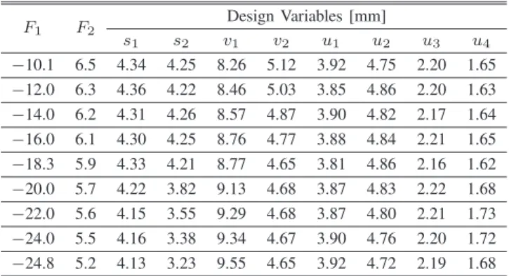
utilized in the refinement procedure (cf. Subsec. 3.3). Subse-quently, response correction technique of Subsec. 2.6 is car-ried out to refine nine designs evenly distributed along the initial Pareto set. The final solutions are obtained after two iterations of refinement procedure each. A comparison of the initial Pareto set based onRsmodel evaluations and its
repre-sentation composed ofRfmodel responses is shown in Fig. 8,
whereas the geometrical details are listed in Table 3. The av-erage gain and reflection varies over the Pareto front from 5.6 dB to 6.4 dB (13%) and from−18.3 dB up to −10 dB (45%), respectively.
Fig. 8. Comparison of the Pareto front obtained from optimizedRs
model (◦)and refined 14Rf model designs ()
Table 3
Refined designs of the optimized planar Yagi-Uda antenna
F1 F2 Design Variables [mm] s1 s2 v1 v2 u1 u2 u3 u4 −10.1 6.5 4.34 4.25 8.26 5.12 3.92 4.75 2.20 1.65 −12.0 6.3 4.36 4.22 8.46 5.03 3.85 4.86 2.20 1.63 −14.0 6.2 4.31 4.26 8.57 4.87 3.90 4.82 2.17 1.64 −16.0 6.1 4.30 4.25 8.76 4.77 3.88 4.84 2.21 1.65 −18.3 5.9 4.33 4.21 8.77 4.65 3.81 4.86 2.16 1.62 −20.0 5.7 4.22 3.82 9.13 4.68 3.87 4.83 2.22 1.68 −22.0 5.6 4.15 3.55 9.29 4.68 3.87 4.80 2.21 1.73 −24.0 5.5 4.16 3.38 9.34 4.67 3.90 4.76 2.20 1.72 −24.8 5.2 4.13 3.23 9.55 4.65 3.92 4.72 2.19 1.68
The total cost of design optimization is about 77Rf
mod-el evaluations (∼29 hours). It includes: acquisition of the low-fidelity simulation data for Kriging model construction (total cost corresponds to about 60Rf model evaluations), and a
total of 27Rfmodel evaluations for high fidelity model
eval-uation and refinement. Similarly to previous cases, the cost of MOEA optimization is neglected.
4.3. Planar Yagi-Uda antenna. Pareto set refinement using Co-kriging. As indicated in Fig. 2, the Pareto set normally occupies a very small fraction of the original design space. Here, in order to allow construction of the initial Kriging surrogate model using reasonably small number of samples (not possible in the original design space), we perform reduc-tion of the design space through finding two extreme points of the Pareto set by means of single-objective optimizations with respect to each considered objectives, one at a time. The reduced space is determined by the following lower and upper frontiers: l = [4.1 3.3 8.3 4.6 3.8 4.7 2.1 1.5]T and
u= [4.4 4.3 9.3 5.2 4.0 4.9 2.3 1.8]T. For the sake of brevity
we omit details related to design space reduction techniques.
Interested reader is referred to the literature (e.g., [32–34]). The Kriging surrogate model is constructed using a set of 500 samples (cf. Subsec. 2.5) and optimized using MOEA. Only the solutions withF1 ≤ −10 dB are considered as relevant
for the refinement (cf. Subsec. 3.3).
The initial Pareto front utilized for the refinement is ob-tained using MOEA ofRsmodel constructed within reduced
solution space. The designs are refined using co-Kriging tech-nique (cf. Subsec. 2.5). Only two iterations of the algorithm were needed to obtain the final Pareto front. A comparison of initial and refined sets is illustrated in Fig. 9. Detailed di-mensions of a 10 selected antenna designs are collected in Table 4. The maximum antenna gain (6.5 dB) comes with the lowest obtained reflection (−10.6 dB) and if varies by 15% along the Pareto optimal set. Moreover, the lowest reflection value is−18 dB (corresponding gain is 5.5 dB).
Fig. 9. Initial Pareto set approximation (◦), final Pareto set obtained after three iterations of the proposed methodology () and 9 selected
high-fidelity model designs () of a planar Yagi-Uda antenna Table 4
Selected designs of the optimized planar Yagi-Uda antenna
F1 F2 Design Variables [mm] s1 s2 v1 v2 u1 u2 u3 u4 −10.6 6.5 4.27 4.26 8.34 5.12 3.87 4.77 2.19 1.72 −11.2 6.4 4.27 4.26 8.32 5.05 3.85 4.83 2.17 1.72 −12.0 6.3 4.25 4.27 8.33 4.93 3.85 4.83 2.17 1.72 −13.0 6.2 4.30 4.19 8.33 4.83 3.89 4.80 2.16 1.73 −13.5 6.0 4.30 4.05 8.38 4.78 3.92 4.76 2.19 1.64 −15.7 5.9 4.21 4.07 8.63 4.66 3.85 4.85 2.14 1.61 −15.9 5.8 4.23 3.83 8.64 4.67 3.84 4.84 2.14 1.62 −16.8 5.7 4.23 3.57 8.77 4.67 3.86 4.82 2.15 1.62 −18.0 5.5 4.14 3.33 9.20 4.73 3.84 4.82 2.23 1.58
The total aggregated cost of the design optimization process corresponds to ∼39 Rf model simulations (∼23
hours). The cost includes: 500×Rc≈21×Rffor a
construc-tion of initial Kriging model and 18×Rf for two iterations
of the Co-kriging algorithm. The cost of MOEA optimization is excluded.
5. Discussion and conclusions
In this paper, we have reviewed two recent techniques for computationally efficient multi-objective design of antennas.
The presented methods utilize an evolutionary algorithm and fast surrogate models constructed using Kriging interpolation of low-fidelity simulation data. Two alternative techniques for refinement of the Pareto optimal set, i.e., response correction, and Co-kriging, are discussed. The methods are illustrated us-ing two exemplary antennas, a three-variable UWB monocone structure and an eight-variable planar Yagi-Uda antenna. Both techniques allow for generating the Pareto front representa-tion at a cost corresponding to several dozens of high-fidelity model evaluations, which is only a small fraction of the cost required by direct multi-objective optimization of EM anten-na models using population-based MOEA, the latter usually being well over several thousands of objective evaluations.
It should also be noted that several techniques for han-dling the design space for the purpose of surrogate model construction have been utilized, including: preparation of sur-rogate model within the original solution space (sufficient for lower-dimensional case), decomposition of the antenna struc-ture into sub-circuits and construction of surrogate models in corresponding subspaces, as well as design space reduction. Slight differences between the Pareto sets obtained during the numerical tests are partially due to utilizing these various ap-proaches.
Although both Pareto set refinement methods generate similar results, the response correction technique is signif-icantly simpler to implement than Co-kriging. The method utilizes output space mapping for a point-by-point refinement of representative antenna designs selected along the Pareto set. The latter approach requires iterative construction and re-optimization of a surrogate model that incorporates both high- and low-fidelity model samples. On the other hand, Co-kriging allows for obtaining more complete Pareto set, not just a few selected designs along it. Also, for the response correction technique, the cost of generating the Pareto set representation increases with the number of required final de-signs, whereas it is essentially constant for the Co-kriging-based method.
The methods discussed in this paper are promising for rapid multi-objective optimization of expensive EM-simulation-based antenna models. However, there are some is-sues that should be addressed by the future research. Perhaps the most important one is design space confinement aimed at identifying the design space region that contains Pareto optimal designs. This is particularly important for handling problems with larger number of variables (>10–15). On the other hand, for certain types of structures (e.g., narrow-band antennas) it might be necessary to apply low-fidelity model correction before attempting to construct the response sur-face approximation surrogate, which because of the original misalignment between EM simulation models of different fi-delities may be too large to be accommodated at the design refinement stage. Addressing the aforementioned issues may results in increasing the range of application of the presented techniques.
Acknowledgements. The authors would like to thank the Computer Simulation Technology AG, Darmstadt, Germany,
for making CST Microwave Studio available. This work was supported in part by the Icelandic Centre for Research (RANNIS), the Grant 130450051, and by the National Sci-ence Centre of Poland, the Grants 2013/11/B/ST7/04325 and 2014/12/ST7/00045.
REFERENCES
[1] H. Schantz,The Art and Science of Ultrawideband Antennas, Artech House, London, 2005.
[2] J. Volakis, C.-C. Chen, and K. Fujimoto, Small Antennas: Miniaturization Techniques and Applications, McGraw-Hill Professional, London, 2010.
[3] F.B. Gross,Frontiers in Antennas: Next Generation Design & Engineering, McGraw-Hill Professional, London, 2011. [4] S. Koziel, F. Mosler, S. Reitzinger, and P. Thoma, “Robust
mi-crowave design optimization using adjoint sensitivity and trust regions”,Int. J. RF and Microwave CAE22, 10–19 (2012). [5] D. Nair and J.P. Webb, “Optimization of microwave devices
using 3-D finite elements and the design sensitivity of the fre-quency response”,IEEE Trans. Magn.39, 1325–1328 (2003). [6] J.I. Toivanen, J. Rahola, R.A.E. Makinen, S. Jarvenpaa, and P. Yla-Oijala, “Gradient-based antenna shape optimization us-ing spline curves”, Ann. Review Progress in Applied Comp. Electromagnetics1, 908–913 (2010).
[7] CST Microwave Studio, ver. 2012, CST AG, Bad Nauheimer Str. 19, D-64289 Darmstadt, 2012.
[8] Ansys HFSS, ver. 14.0 (2012), ANSYS, Inc., Southpointe 275 Technology Drive, Canonsburg, PA 15317.
[9] J.W. Bandler, Q.S. Cheng, S.A. Dakroury, A.S. Mohamed, M.H. Bakr, K. Madsen, and J. Søndergaard, “Space mapping: the state of the art”,IEEE Trans. Microwave Theory Tech.52, 337–361 (2004).
[10] S. Koziel, S. Ogurtsov, and S. Szczepanski, “Rapid antenna de-sign optimization using shape-preserving response prediction”, Bull. Pol. Ac.: Tech.60 (1), 143–149 (2012).
[11] S. Koziel and S. Ogurtsov, “Rapid design optimization of an-tennas using space mapping and response surface approxi-mation models”, Int. J. RF & Microwave CAE21, 611–621 (2011).
[12] I. Couckuyt, S. Koziel, and T. Dhaene, “Surrogate modeling of microwave structures using kriging, co-kriging and space mapping”,Int. J. Numerical Modelling: Electronic Devices and Fields26, 64–73 (2013).
[13] S. Koziel and J.W. Bandler, “Accurate modeling of microwave devices using kriging-corrected space mapping surrogates”, Int. J. Numerical Modelling25, 1–14 (2012).
[14] S. Koziel and S. Ogurtsov, “Model management for cost-efficient surrogate-based optimization of antennas using variable-fidelity electromagnetic simulations”,IET Microwaves Ant. Prop.6, 1643–1650 (2012).
[15] S. Koziel and S. Ogurtsov, Antenna Design by Simulation-Driven Optimization, Springer, Berlin, 2014.
[16] S. Koulouridis, D. Psychoudakis, and J. Volakis, “Multiobjec-tive optimal antenna design based on volumetric material opti-mization”,IEEE Tran. Antennas Propag.55, 594–603 (2007). [17] Y. Kuwahara, “Multiobjective optimization design of Yagi– Uda antenna”, IEEE Tran. Antennas Propag. 53, 1984–1992 (2005).
[18] M. John and M.J. Ammann, “Antenna optimization with a computationally efficient multiobjective evolutionary algo-rithm”,IEEE Tran. Antennas Propag.57, 260–263 (2007).
[19] T. Maruyama, K. Yamamori, and Y. Kuwahara, “Design of multibeam dielectric lens antennas by multiobjective optimiza-tion”,IEEE Tran. Antennas Propag. 57, 57–63 (2007). [20] N. Jin and Y. Rahmat-Samii, “Advances in particle swarm
optimization for antenna designs: real-number, binary, single-objective and multisingle-objective implementations”,IEEE Tran. An-tennas Propag. 55, 556–567 (2007).
[21] B. Aljibouri, E.G. Lim, H. Evans, and A. Sambell, “Multi-objective genetic algorithm approach for a dual-feed circular polarised patch antenna design”,Electronic Letters36, 1005– 1006 (2000).
[22] S. Chamaani, M.S. Abrishamian, and S.A. Mirtaheri, “Time-domain design of UWB Vivaldi antenna array using multi-objective particle swarm optimization”, IEEE Antennas and Wireless Prop. Lett.9, 666–669 (2010).
[23] H. Choo, R.L. Rogers, and H. Ling, “Design of electrically small wire antennas using a pareto genetic algorithm”,IEEE Trans. Antennas Prop.53, 1038–1046 (2005).
[24] S. Koziel and S. Ogurtsov, “Multi-objective design of anten-nas using variable-fidelity simulations and surrogate models”, IEEE Trans. Antennas Prop.61, 5931–5939 (2013).
[25] S. Koziel, A. Bekasiewicz, I. Couckuyt, and T. Dhaene, “Effi-cient multi-objective simulation-driven antenna design using Co-kriging”, IEEE Tran. Antennas Propag. 62, 5900–5905 (2014).
[26] M.C. Kennedy and A. O’Hagan, “Predicting the output from complex computer code when fast approximations are avail-able”,Biometrika87, 1–13 (2000).
[27] K. Deb,Multi-Objective Optimization Using Evolutionary Al-gorithms, John Wiley & Sons, New York, 2001.
[28] S. Koziel, and S. Ogurtsov, “Model management for cost-efficient surrogate-based optimization of antennas using variable-fidelity electromagnetic simulations”,IET Microwaves Antennas Prop.6, 1643–1650 (2012).
[29] T.W. Simpson, J. Peplinski, P.N. Koch, and J.K. Allen, “Meta-models for computer-based engineering design: survey and
recommendations”,Engineering with Computers 17, 129–150 (2001).
[30] A.I. Forrester, A. Sobester, and A.J. Keane, “Multi-fidelity op-timization via surrogate modelling”,Proc. Royal Society463, 3251–3269 (2007).
[31] B. Beachkofski and R. Grandhi, “Improved distributed hyper-cube sampling”,American Institute of Aeronautics and Astro-nauticsAIAA 2002, 1274 (2002).
[32] A. Bekasiewicz, S. Koziel, and W. Zieniutycz, “Design space reduction for expedited multi-objective design optimization of antennas in highly-dimensional spaces”, in Solving Computa-tionally Extensive Engineering Problems: Methods and Appli-cations, Springer, Berlin, 2014.
[33] S. Koziel, A. Bekasiewicz, and W. Zieniutycz, “Expedite EM-driven multi-objective antenna design in highly-dimensional parameter spaces”,IEEE Antennas and Wireless Propagation Letters13, 631–634 (2014).
[34] A. Bekasiewicz, S. Koziel, and L. Leifsson, “Low-cost EM-simulation-driven multi-objective optimization of antennas”, Int. Conf. Computational Science, inProcedia Computer Sci-ence29, 790–799 (2014).
[35] S. Koziel, Q.S. Cheng, and J.W. Bandler, “Space mapping”, IEEE Microwave Magazine9, 105–122 (2008).
[36] Y. Qian, W.R. Deal, N. Kaneda, and T. Itoh, “Microstrip-fed quasi-Yagi antenna with broadband characteristics”, Electron-ics Letters34, 2194-2196 (1998).
[37] J. Kwiecien and B. Filipowicz, “Comparison of firefly and cockroach algorithms in selected discrete and combinatorial problems”,Bull. Pol. Ac.: Tech.62 (4), 797–804 (2014). [38] T. Lewinski, S. Czarnecki, G. Dzierzanowski, and T. Sokol,
“Topology optimization in structural mechanics”, Bull. Pol. Ac.: Tech.61 (1), 23–37 (2013).
[39] B. Blachowski and W. Gutkowski, “Graph based discrete opti-mization in structural dynamics”, Bull. Pol. Ac.: Tech.62 (1), 91–102 (2014).