Miikka Rytty
AFFINE MULTI-FACTOR SHORT-RATE MODELS IN TERM STRUCTURE MODELING
Master’s Thesis Department of Finance
Unit
Department of Finance
Author
Miikka Rytty
Supervisor
Professor Jukka Perttunen
Title
Affine multi-factor short-rate models in term structure modeling
Subject
Finance
Type of the degree
Master’s Thesis Time of publication May 2019 Number of pages 177 Abstract
This thesis gives an overview of short-rate models in term structure modeling of interest rates. The focus is in simple preference-free models with affine term structures. The thesis also shows how these models can be extended to cover credit spreads over the risk-free interest rate. The empirical section analyzes how well these models can be applied to recent interest rate data. While short-rate models are still used, more recent market models have eclipsed them in pricing of complex derivatives. The previous literature in short-rate modeling has been mainly conducted before the financial crisis of 2007-08 and there is very little literature on comparing how well these models perform in the current market structure which features negative interest rates.
The first chapters give an overview of arbitrage-free pricing methodology of contingent claims and short-rate modeling of interest rates and credit spreads. These chapters present analytical pricing formulas for zero-coupon bonds with and without credit risk and semi-analytical pricing method for options on zero-coupon bonds in simple preference-free affine multi-factor short-rate models. The main finding of the empirical study shows that single-factor models do not fit the recent market data. For multi-factors models, the results were not conclusive. The calibration of multi-factor models is very hard multi-dimensional optimization problem with heavy computational burden. While the quality of the multi-factor model calibrations was mostly lacking, the mixed results suggest that insufficient computing power might be cause. The rationale for this conclusion was that the calibration algorithm could not replicate previous calibration results when a different starting
population was used in optimization. It seems that there were not enough computational resources to guarantee that stochastic optimization algorithm was able to find optimal parameter values.
Based on the findings of the empirical study, it seems that multi-factor short-rate models with affine term structure can be used in term structure modeling but with caveats. The whole discount curve from over-night rate to the maturity of 30 years seems to be too complex for these models but shorter sections worked much better and optimization and the computational burden may not be ignored in a more serious calibration attempt.
Keywords
Short-rate, interest rate modeling, preference-free affine models, credit risk
CONTENTS
1 Introduction 8
1.1 Overview of the arbitrage-free asset pricing . . . 8
1.1.1 Arbitrage-free interest rate models . . . 9
1.1.2 Intensity based modeling of credit risk . . . 12
1.2 Overview of the thesis . . . 12
1.3 Fixed notation . . . 16
2 Idealized rates and instruments 17 2.1 Fundamental rates and instruments . . . 17
2.1.1 Short-rate, idealized bank account and stochastic discount factor 17 2.1.2 Zero-coupon bond . . . 18
2.1.3 Simple spotL(t,T)andk-times compounded simple spot rate 18 2.1.4 Forward rate agreement . . . 19
2.2 Interest rate instruments . . . 22
2.2.1 Fixed leg and floating leg . . . 22
2.2.2 Coupon bearing bond . . . 23
2.2.3 Vanilla interest rate swap . . . 23
2.2.4 Overnight indexed swap . . . 24
2.2.5 Call and put option and call-put parity . . . 24
2.2.6 Caplet, cap, floorlet and floor . . . 24
2.2.7 Swaption . . . 26
2.3 Defaultable instruments and credit default swaps . . . 27
2.3.1 DefaultableT-bond . . . 27
2.3.2 Credit default swap . . . 28
3 An introduction to arbitrage pricing theory 30 3.1 Discrete one period model . . . 30
3.1.1 The first fundamental theorem of asset pricing in discrete one period model . . . 31
3.1.2 The second fundamental theorem of asset pricing in discrete
one period model . . . 35
3.2 Arbitrage theory in continuous markets . . . 38
3.2.1 Risk-free measure . . . 42 3.2.2 Black-Scholes–model . . . 43 3.2.3 Black-76–model . . . 46 3.2.4 T-forward measure . . . 47 3.2.5 Change of numéraire . . . 48 4 Short-rate models 50 4.1 Introduction to short-rate models . . . 50
4.1.1 Term-structure equation . . . 50
4.1.2 Fundamental models . . . 52
4.1.3 Preference-free models . . . 53
4.2 One-factor short-rate models . . . 54
4.2.1 Affine one-factor term-structures models . . . 54
4.2.2 Vašíˇcek–model . . . 56
4.2.3 Cox-Ingersol-Ross–model (CIR) . . . 60
4.3 Multi-factor short-rate models . . . 62
4.3.1 SimpleA(M,N)+–models . . . 62
4.4 Dynamic extension to match the given term-structure . . . 64
4.4.1 Vašíˇcek++–model . . . 68
4.4.2 CIR++–model . . . 70
4.4.3 G2++–model . . . 70
4.5 Option valuation using Fourier inversion method . . . 71
5 Intensity models 76 5.1 Foundations of intensity models . . . 76
5.1.1 Introduction . . . 76
5.1.2 The credit triangle . . . 80
5.2 Pricing . . . 82
5.2.1 The protection leg of a credit default swap . . . 84
5.2.2 The premium leg of a credit default swap . . . 85
5.3 The assumption that the default is independent from interest rates . . . 87
6 Empirical work 93
6.1 Research environment . . . 93
6.2 Stationary calibration . . . 94
6.2.1 Models without credit risk . . . 94
6.2.2 Models with credit risk . . . 102
6.3 Dynamic Euribor calibration without credit risk . . . 104
7 Summary 111 A Mathematical appendix 114 A.1 Characteristic function and Fourier transformation . . . 114
A.2 Radon-Nikodým-theorem and the change of measure . . . 115
A.3 Conditional expectation . . . 116
A.4 Filtrations and martingales . . . 120
A.5 A stopping time and localization . . . 120
A.6 Brownian motion . . . 121
A.7 Itô-integral . . . 124
A.8 Itô processes and Itô’s lemma . . . 125
A.9 Geometric Brownian motion . . . 127
A.10 Girsanov’s theorem . . . 127
A.11 Martingale representation theorem . . . 129
A.12 Feynman-Kac theorem . . . 130
A.13 Partial information . . . 130
A.14 Doubly stochastic default time . . . 132
A.15 A gaussian calculation . . . 134
A.16 Differential evolution . . . 135
B Charts and graphs 137 B.1 Graphical presentation of the initial curve data . . . 138
B.2 Comparison of actual inferred rates and calibrated model prices with-out default risk . . . 143
B.3 Comparison of different calibrations between models without default risk . . . 155
B.4 Model parameters for affine models without default risk . . . 158
B.5 Comparison of parameters for affine models without default risk be-tween different calibration attempts . . . 159
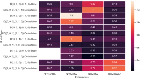
B.6 Actual prices and calibrated prices of default models . . . 165
B.8 Comparison of calibrated parameters for affine models with default risk 170 B.9 Dynamic Euribor calibration without credit risk . . . 173
LIST OF FIGURES
1.1 OTC derivatives notional amount outstanding. Source: BIS 2018 . . . 10
1.2 OTC derivatives gross market values. Source: BIS 2018 . . . 10
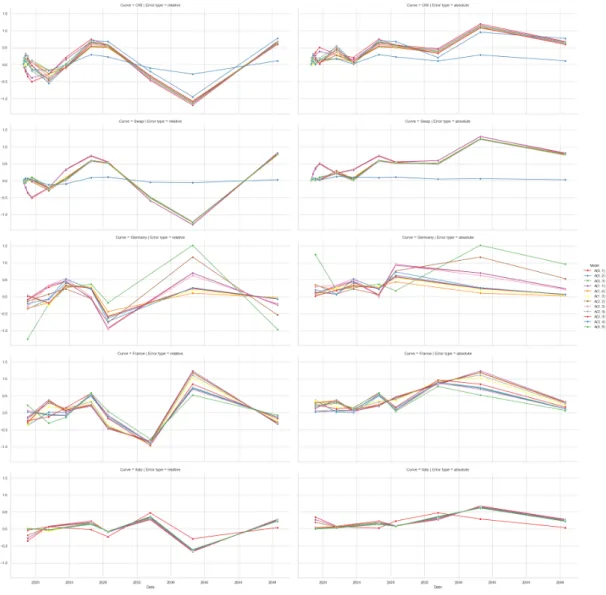
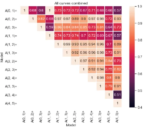
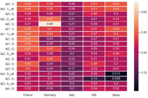
6.1 Calibration errors for models without credit risk . . . 98
6.2 Error correlations for models without credit risk . . . 99
6.3 Mean absolute calibration error for models without credit risk . . . . 100
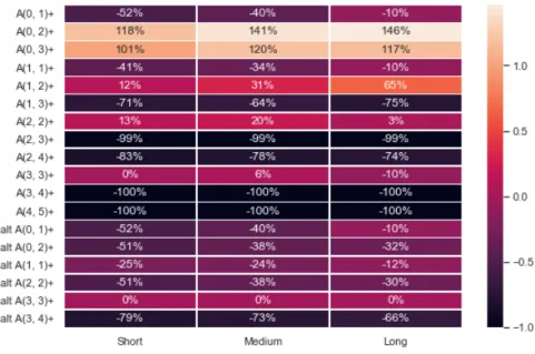
6.4 Relative pricing errors of sample caps compared to prices given by OIS A(3,4)+-model . . . 101
6.5 Relative pricing errors of sample caps compared to prices given by swapA(3,3)+-model . . . 102
6.6 Mean absolute calibration error for models with default risk . . . 103
6.7 Euribor rates from February 26, 2004 to January 26, 2019 . . . 104
6.8 Implied Euribor discount factors from February 26, 2004 to January 26, 2019 . . . 105
6.9 Correlation of Euribor rate changes from February 26, 2004 to January 26, 2019 . . . 105
6.10 Euribor rate and discount curves . . . 106
6.11 Euribor rate and discount curves . . . 107
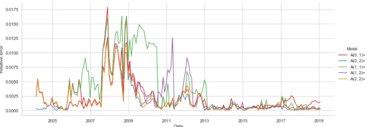
6.12 Time series of mean absolute relative errors in Euribor fitting. . . 108
6.13 Errors in Euribor fitting by model and maturity. . . 109
6.14 Errors in Euribor fitting by time period. . . 110
B.1 Interpolated interest rates and instantaneous forward rate curves . . . 138
B.2 Interpolated interest rates . . . 139
B.3 Theoretical zero coupon bond prices inferred from the rate data by using different interpolation methods . . . 140
B.4 Theoretical zero coupon bond prices inferred from the rate data . . . . 141
B.5 Calibrated rates by modelA(0,1) . . . 143
B.6 Calibrated rates by modelA(1,1) . . . 144
B.8 Calibrated rates by modelA(1,2) . . . 146
B.9 Calibrated rates by modelA(2,2) . . . 147
B.10 Calibrated rates by modelA(0,3) . . . 148
B.11 Calibrated rates by modelA(1,3) . . . 149
B.12 Calibrated rates by modelA(2,3) . . . 150
B.13 Calibrated rates by modelA(2,4) . . . 151
B.14 Calibrated rates by modelA(3,3) . . . 152
B.15 Calibrated rates by modelA(3,4) . . . 153
B.16 Calibrated rates by modelA(4,5) . . . 154
B.17 Comparison of alternative calibrations for single factor models . . . . 155
B.18 Comparison of alternative calibrations for 2-factor models . . . 156
B.19 Comparison of alternative calibrations for multifactor models . . . 157
B.20 Calibration and actual prices for OIS and swap rate . . . 165
B.21 Calibration and actual prices for OIS and Italy . . . 166
B.22 Calibration and actual prices for Germany and France . . . 167
B.23 Calibration and actual prices for Germany and Italy . . . 168
B.24 Relative calibration errors for credit risk models . . . 169
B.25 Absolute relative calibration errors for credit risk models . . . 170
LIST OF TABLES
6.1 Number of parameters per model . . . 96
B.1 Overnight index swap . . . 158
B.2 Swap . . . 158
B.3 Germany . . . 158
B.4 France . . . 158
B.5 Italy . . . 158
B.6 Overnight index swap and swap curve . . . 170
B.7 Overnight index swap and Italy . . . 171
B.8 Germany and Italy . . . 171
1. INTRODUCTION
1.1. Overview of the arbitrage-free asset pricing
What is an appropriate price of an asset? Financial assets, which are contracts over other assets, are often homogeneous and standardized. Intuitively their prices should mainly depend on investors’ preferences over the distributions of future returns. In-vestors have different preferences. Risk appetite, regulatory requirements, investment horizons and business concerns differentiates them. Secondly, history has showed that predicting the future is difficult and, as a corollary, detailed prediction of price be-havior should be also hard. Without auguries, the derivation of exact probabilities is impossible.
According to Cochrane (2009), "asset pricing theory tries to understand the prices or values of claims to uncertain payments (p. xiii)". Asset pricing theory has two main approaches, absolute and relative pricing. Absolute pricing tries to model sources of economic risks and/or underlying preferences, and derive prices from these. The canonical examples are CAPM and other equilibrium models. In contrast, relative pric-ing does not try the model the whole investment universe. In relative prices, some asset prices are exogenous and other assets are priced relative to these. Black-Scholes–model (Black and Scholes 1973) is canonical example of this approach. The demarcation of these approaches is not clear-cut. CAPM assumes the equilibrium prices as given and Black-Scholes–model makes a fundamental assumption about the distribution of asset returns. (Cochrane 2009, pp. xiii–xiv)
The relative pricing approach is often called as arbitrage pricing methodology. The common theme in these models is that we make an assumptions about the underlying distribution of the exogenous prices. If the market is arbitrage-free, then these exoge-nous prices contain meaningful information about probabilities for different outcomes probability distribution. Thus we do not try to derive actual probability distribution, but we construct a new probability measure, which is commonly called as the equiva-lent martingale measure (EMM). These implied distributions are then used to construct replicating portfolios. By a construction of a perfect hedge, preferences do not affect the price of a replicating portfolio.
The seed of the arbitrage pricing theory is usually attributed to the thesis by Bache-lier (1900). But the research by Jovanovic and Le Gall (2001) suggest that BacheBache-liers work was antecedent by another French Regnault (1863). The insight of these early pioneers was not try to outguess the market but the idea was model the price
move-ments by Brownian motion1 and use the distribution to price the derivative contract.
Although the work of Bachelier was temporarily forgotten, it resurfaced in the 1950’s and influenced a host of work (Samuelson 1973). Thus Regnault and Bachelier can be also seen as the forefathers of the efficient-market hypothesis which was largely developed in modern sense by Fama (1965) and Samuelson (1965a).
These early modern attempts to price options were not satisfactory even to the
authors who derived them2 until the seminal work by Black and Scholes (1973). The
major insight in this and subsequent work was that, in certain idealized frictionless market model, the cash flow of the option could be perfectly replicated by trading the underlying stock and a risk-free bond. Since there was no practical difference in executing this trading strategy and owning the option, there was a unique no-arbitrage price for the option. This price depends neither the risk aversion of the inverstor nor his views of the market (expect for the volatility of stock price).
The mathematical formulation in Black and Scholes (1973) was lacking. Accord-ing to Musiela and Rutkowski (2005, p. 129), it was Bergman (1982) who first noted that the trading strategy used by Black and Scholes (1973) was neither risk-free nor self-financing. The modern arbitrage asset pricing theory was formalized by Harrison and Kreps (1979) in discrete time and Harrison and Pliska (1981) in continuous time (see also Harrison and Pliska (1983)). Several authors have expanded these works and Delbaen and Schachermayer (1998) (and references within) present one version of the theory in very general a semi-martingale setting.
1.1.1. Arbitrage-free interest rate models
The demand for accurate pricing models for interest rate derivatives is great, as the po-sitions are large. According to BIS (2018), the outstanding amount of over the counter interest rate derivatives was over 436.8 trillion USD. However, since many of the po-sitions are overlapping, gross market value gives a better estimate of the actual size of derivative positions. This gross market value was about 6.84 trillion. Figures 1.1 and 1.2 show the development OTC derivative market segments.
1The problem with Brownian motion is that with non-zero probability the price will be negative
given enough time. A more valid approach is to use geometric Brownian motion which do not have this problem. But geometric Brownian motion is still continous so it will not model the jumps in the price process.
Figure 1.1: OTC derivatives notional amount outstanding. Source: BIS 2018
Figure 1.2: OTC derivatives gross market values. Source: BIS 2018
A vast literature exist to explain the mechanics driving the term-structure of inter-est rates. Short-rate modeling began under this framework and was based on macro-economical argumentation. According to Duffie (2010, p. 161), the earliest example of markovian term-structure model is by Pye (1966). His approach influenced Mer-ton (1974), a paper which contains an example of gaussian short-rate model. The first relevant short-rate model is the famous Vašíˇcek–model by Vašíˇcek (1977). Another widely used short-rate model is CIR–model by Cox, Ingersoll Jr, and Ross (1985). Since the original formulation of these models are based on economic equilibrium argumentation, they are often called either equilibrium or fundamental models and risk-preferences have to be explicitly formulated and they influences prices. Although fundamental models may have economically sound argumentation, their basic problem is practical impossibility to fit them to the observed interest-rate structure.
These early models can be also cast in arbitrage pricing framework, but we lose the economic justification behind the interest rate process. Arbitrage-free short-rate mod-eling just assumes that the interest rates are generated by a given exogenous stochastic process, a short-rate. This rate is mathematically modeled by an Itó-process. Observed
rates are then stochastic integrals of this short rate. By this approach, pricing of inter-est rate derivatives leads to solving stochastic differential equations. When the short-rate model has constant parameters, then the observed interest-short-rate structure may not be matched. Ho and Lee (1986) introduced a short-rate model with time-varying pa-rameter, which can be chosen to fit the observed term-structure. Vašíˇcek–model was extended with time-varying parameters in J. Hull and White (1990).
Since short-rate models capture only a point, they have hard time capturing the complex dynamics of the term-structures. For example, we later show that in single-factor affine term-structure models rates of different maturities are perfectly correlated. An alternative to the short-rate approach is to directly model the entire term structure of interest rates. An early successor was HJM–framework (introduced in Heath, Jar-row, and Morton 1990 and Heath, JarJar-row, and Morton 1992), which models the entire forward rate process. It should be noted Ho-Lee and Hull-White models can be cast as special cases of HJM model. A major problem for general HJM models is that these are not necessary markovian (Ritchken and Sankarasubramanian 1995).
Nowadays so called market models are widely used in pricing. According to Wu (2009, p. 182), traders had assumed that LIBOR and swap rates were log-normal
pro-cesses and used Black’s formula3 to quote volatility when pricing caps and swaptions
since the early 1990’s. Theoretical justification for these practices were finally found in 1997 by a series of articles by Brace, Gatarek, and Musiela 1997, Miltersen, Sand-mann, and Sondermann (1997) and Jamshidian (1997). Market models use LIBOR (or other market interest rates) as the fundamental objects and assume that they can be modeled as log-normal processes. Thus they are often called as LIBOR models. The main feature of market models is that cap and swaption pricing is given by Black’s for-mula and they can be made to fit given term-structure and volatility structures. Since the LIBOR rates follow log-normal rates, these models have to be extended to handly negative interest rate. This is often done by modeling a shifted log-normal process. A popular extension of market model is SABR volatility model by Hagan, Kumar, Lesniewski, and Woodward (2002).
The global financial crisis of 2007-08 has had a major impact on interest-rate mod-eling. One of the significant additions is the multi-curve framework (Mercurio (2009)). Before the crisis, the spread between overnight indexed swap (OIS) and LIBOR curves were minimal and LIBOR curve was both the discounting and forward rate generating curve. During the crisis, this spread widened dramatically and afterwards it has been necessary the model these curves separately.
1.1.2. Intensity based modeling of credit risk
An early example of credit risk modeling is Merton (1974), which uses Black-Scholes– model to price corporate debt subject to credit risk. In Merton’s model corporate assets are assumed to follow geometric brownian motion and the corporate debt consists of single zero-coupon bond. Now the equity can be seen as a call option on corporate assets with the strike price of the face value of a bond at the maturity. Thus the equity price is given by the Black-Scholes formula and the bond price is the difference of asset and equity values. Merton (1974) is extended by proprietary Moody’s KMV model.
An alternative to the structural credit models are dynamic models. One approach is to use so called intensity based modeling of default. In this framework, the default time
is a stopping time with a intensity process4. This intensity process may be influenced
by properties of economy or the underlying entity. In the arbitrage-free settings inten-sity may be modeled by either Poisson or Cox processes. This approach was pioneered by Artzner and Delbaen (1995), Jarrow and Turnbull (1995) and Lando (1998).
The popularity intensity based modeling is due to synergies with short-rate mod-els of interest rates. When set-up correctly, the default intensity process is the credit spread process. Then the pricing of debt and related instruments can be made using the machinery developed for the short-rate processes. J. Schönbucher (2001) has extended market models to cover credit intensity modeling.
After the global financial crisis of 2007-08, the credit risk modeling has gained importance. For example, Basel III framework requires that the prices of unsecured
derivative positions has to be corrected with CVA5, which accounts for the
counter-party credit risk (BIS 2015).
1.2. Overview of the thesis
The purpose of this thesis is to have a rough overview arbitrage-free pricing method-ology and affine short-rate processes used in interest rate modeling and credit risk. Although short-rate models have been eclipsed by market models, they still have their uses in risk management, portfolio management and scenario planning.
As the short-rate models were developed before global financial crisis of 2007-08, we test how well they can be fitted to the post-crisis interest rate data. We also try to test calibrate a combined short-rate and credit spread model to post-crisis bond price data.
4See chapter 5 and section A.5.
Chapter 2
Chapter 2 gives a basic overview of the common interest rates and financial instru-ments.
Chapter 3
Chapter 3 gives a very brief introduction to arbitrage pricing theory. We first develop discrete one period model in order to highlight the basic concepts of arbitrage pricing such as justification behind martingale measures and laws of asset pricing. This treat-ment is based on Björk (2004, pp. 5–34). All the proofs are detailed as we feel that they give insight to martingale measures.
After that the arbitrage pricing in continuous markets is overviewed. This treatment is not rigorous. Measure theoretical justifications and arguments are simply omitted although some basic results are presented in Appendix A.
While not strictly necessary for the empirical work in this thesis, the arbitrage pricing theory is essential for understanding the peculiarities in interest rate and credit spread modeling.
Chapter 4
Chapter 4 starts with the derivation of term-structure equation and the overview of the fundamental and preference-free models. We have a brief overview of the single-factor Vašíˇcek and CIR–models.
We also cover multi-factor affineA(M,N)–models, which are a combination ofM
Vašíˇcek and N−M CIR–models. The Gaussian processes can be chosen to be
cor-related but square-root processes has to be uncorcor-related. The theory of affine term-structure models was developed for example in Brown and Schaefer (1994), Duffie and Kan (1994) and Duffie and Kan (1996). The main advantage of these affine mod-els is that they have analytical bond prices which make calibration by term-structure
easy. By dynamic extension shifting6, we even could make sure that term-structures fit
perfectly. Many of these models also have analytical bond option prices, which allows us to price caps and floors and for single factor models, this allows also easy pricing of swaptions. Therefore they can be easily fit to volatility structures also. Even if the model does not have a bond option pricing formula, we may use Fourier
transforma-tions to have semi-analytical pricing of bond optransforma-tions7.
6See Brigo and Mercurio (2001) and section 4.4. 7See Heston (1993) and section 4.5.
All the simple preference-free models models8 covered in Chapter 4 see imple-mentation in the empirical work in Chapter 6.
Chapter 5
Chapter 5 is an overview of default intensities in credit risk modeling. We show how
a Cox process9can be used to extended the machinery of short-rate interest rate
mod-eling to model credit spreads. In order to do this, we show how to price discounted cash flows that depend on timing of a default event, where both short-rate and default intensity are stochastic in nature. We develop model-independent pricing formulas of defaultable zero-coupon bonds. Although credit default swaps are not covered in the emperical work of Chapter 6, we also show how easily these methods can be used to the price credit default swaps.
There is also an exposition covering on how the multi-factor affineA(M,N)–models
of Chapter 4 can be extended to model both interest rates and default intensities. In the empirical chapter, we try to calibrate these models to market data.
Chapter 6
Chapter 6 presents the methods and results from the empirical work done in this thesis. We test some of the methods develop in earlier chapters. In order to find suitable initial starting value for descending optimization algorithm, we tried to scan the problem space with a differential evolution (DE) algorithm. Due to computational limitations, the sample sizes were small compared to the dimension of the problem space. As such, the algorithm did not produce consistent results.
Simple affine models were fitted to various interest rate and yield curves with and without default risk. Fittings of these curves proved to be challenging for the models as the maturities ranged from overnight rates (or 6-month rates) to 30-year rates. No model provided satisfactory fitting in every case. Fitting done by models with credit risk component proved bad overall. However, due to the problems with optimization algorithm, we can not decisively rule that the models will provide bad fits with the used data.
Dynamic fitting of Euribor rates ranging from 1-week rate to 1-year rate was also attempted to single factor models. Depending on the time-period, the fits ranges from horrible to rather satisfactory. As the short end of the rate curve has been rather flat after 2014, calibrated curves had very little errors.
8See section 4.1 for introduction to these models.
9Cox process is also called as doubly stochastic process, since in addition to the stochastic stopping
Due to data and computational limitations, fitting to the volatility structures was not attempted.
The code with the Jupyter notebook used in analysis can be found athttps://gi
thub.com/mrytty/gradu-public(Rytty (2019)).
Appendices A and B
Appendix A is a brief review of mathematical machinery and methods needed in the earlier chapters.
Appendix B presents some additional data charts and tables from the empirical work.
1.3. Fixed notation
The following notation will be fixed.
∆(t,T) Day count convention fraction between the datest <T. r(t) Short-rate at the timet.
B(t) The value of an idealized bank account at the timet.
D(t,T) Stochastic discount factor between the datest,T.
p(t,T) The price ofT-bond (zero coupon bond with the maturityT) at the timet.
L(t,T) Simple spot rate between datest andT
Lk(t,T) k-times compounded simple spot rates between datestandT
FRA(t,T,S,K) The price of a forward rate agreement at the time t, where K is the
fixed price and the interest is paid between the datesT <S.
L(t,T,S) Simple forward rate at the timet between datesT andS f(t,T) Instantaneous forward rate at the timet for dateT.
Fut(t,T,S) Futures rate at the timetbetween datesT andS.
d(t,T) The price of defaultableT-bond (zero coupon bond with the maturityT) at the
timet.
ZBC(t,S,T,K) The price of call option at the timetmaturing atSwritten onT-bond.
ζ The time of a default.
LGD The loss given the default (LGD) of a contract.
REC The recovery value of a contract.
CDSpro(t) The value of a protection leg of a credit default swap.
CDSpre(t,C) The value of a premium leg of a credit default swap with a coupon rate
2. IDEALIZED RATES AND INSTRUMENTS
In this chapter we review idealized versions of interest rates and derivatives of interest rates. By idealized, we mean that the instruments are simplied for analytical purposes. For example, there is no lag between trade and spot date or expiry and delivery date. Neither we do not use funding rate that is separate form the market rates. The treat-ment is standard and is based mainly on Brigo and Mercurio (2007, pp. 1–22) unless otherwise noted.
In the following, we assume that 0<t<T are points of time and∆(t,T)∈[0,∞)
is the day count convention between the points t and T. We explicitly assume that
∆(t,T)≈T−twhent≈T.
2.1. Fundamental rates and instruments
2.1.1. Short-rate, idealized bank account and stochastic discount factor
When making calculations with idealized bank account, it is customary to assume that the day count-convention∆(t,T) =T−tas this will simplify the notation. An idealized
bank account is an instrument with the value
B(t) =exp t Z 0 r(s)ds (2.1.1)
wherer(t) is the short-rate rate. The short-rater(t)may be non-deterministic but we assume that it is smooth enough so that the integral can be defined in some useful sense. We note thatB(0) =1. Ifδ >0 is very small andr(t)is a smooth function, then
t+δ
Z
t
r(s)ds≈r(t)δ (2.1.2)
and we see that the first-order expansion of exponential function yields
Thus the short-rate can be seen as continuous interest rate intensity. Short-rate is purely theoretical construction which can be used to price financial instruments.
Now we may define a stochastic discount factorD(t,T)from timet toT as
D(t,T) = B(t) B(T)=exp − T Z t r(s)ds . (2.1.4)
Ifr(t)is a random variable, thenB(t)andD(t,T)are stochastic too.
2.1.2. Zero-coupon bond
A promise to pay one unit of currency at timeT is called aT-bond. We shall assume
that there is no credit risk for these bonds. We further assume that the market is liquid and bond may be freely bought and sold at the same price, furthermore short selling
is allowed without limits or extra fees. The price of this bond at timet is denoted by
p(t,T)and so p(t,T)>0 and p(T,T) =1.
AsD(0,t)is guaranteed to pay one unit of currency at the timet, we see that in this caseD(0,t) =p(0,t). We note that if the short-rater(t)is deterministic, then
D(0,t) = 1
B(t) (2.1.5)
is deterministic too. We see that if short-rater(t)is deterministic, thenD(t,T) =p(t,T)
for all 0≤t≤T. But this does not hold ifr(t)is truly stochastic.
2.1.3. Simple spotL(t,T)andk-times compounded simple spot rate
The simple spot rateL(t,T)is defined by
L(t,T) = 1−p(t,T)
∆(t,T)p(t,T), (2.1.6)
which is equivalent to
1+∆(t,T)L(t,T) = 1
p(t,T). (2.1.7)
Fork≥1, thek-times compounded interest rate fromt toT is
Lk(t,T) = k p(t,T)
1
k∆(t,T)
which is equivalent to p(t,T) 1+L k(t,T) k k∆(t,T) =1. (2.1.9) As (1+x k) k−→ ex (2.1.10) whenk−→∞, then 1+L k(t,T) k k∆(t,T) −→e∆(t,T)r(t,T), (2.1.11) whereLk(t,T)−→r(t,T)whenk−→∞.
2.1.4. Forward rate agreement
A forward rate agreement (FRA) is a contract that pays
∆K(t,T)K−∆(t,T)L(t,T) (2.1.12)
at the time T. Here we assume that the contact is made at the present time 0 and
0<t <T, but this assumption is made just to keep the notation simplier. HereKis an interest rate that is fixed at time 0,∆K is the day count convention for the this fixed rate
andL(t,T)is the spot rate from timet toT (which might not be know at the present).
The price of a FRA at the times≤tis denoted by FRA(s,t,T,K). Now
FRA(t,t,T,K) =p(t,T) (∆K(t,T)K−∆(t,T)L(t,T)). (2.1.13)
In order to price a FRA at different times, we consider a portfolio of one longT
-bond andxshortt-bonds. The value of this portfolio at the present isV(0) =p(0,T)−
xp(0,t)and we note that the portfolio has zero value if
x= p(0,T)
At the timet, the portfolio has value V(t) =p(t,T)−x (2.1.15) =p(t,T) 1− x p(t,T) (2.1.16)
where p(t,T)is known and
1+∆(t,T)L(t,T) = 1 p(t,T) =y(t,T). (2.1.17) We defineK∗(x) =x−1. Thus 1− x p(t,T) =x 1 x− 1 p(t,T) (2.1.18) =x(K∗(x)−y(t,T)) (2.1.19)
and this implies that
V(t) =xp(t,T) (K∗(x)−y(t,T)). (2.1.20)
Without arbitrage
V(T) =x(K∗(x)−y(t,T)) (2.1.21)
=x(K∗(x)−1−∆(t,T)L(t,T)) (2.1.22)
We note that at the time 0,K∗(x)is a known yield but y(t,T)is an unknown yield if
p(t,T)is not deterministic. Now if
K= 1 ∆K(t,T) (K∗(x)−1) (2.1.23) = 1 ∆K(t,T) 1 x−1 (2.1.24)
the given portfolio can be used to replicate the cash flows of the FRA and
xFRA(s,t,T,K) =V(s). (2.1.25)
If
x= p(0,T)
thenV(0) =0 and K= 1 ∆K(t,T) p(0,t) p(0,T)−1 (2.1.27) = ∆(t,T) ∆K(t,T) L(t,T). (2.1.28)
We see that the forward rate and the rate that defines FRA with zero present value are
essentially the same. Thus we define that the forward rate at the timet from timeT to
Sis L(t,T,S) = 1 ∆(T,S) p(t,T) p(t,S)−1 . (2.1.29)
Since∆(T,S)≈S−T whenT ≈S, we have that
L(t,T,S) = 1 ∆(T,S) p(t,T) p(t,S)−1 (2.1.30) ≈ 1 p(t,T) p(t,T)−p(T,S) S−T (2.1.31) and therefore L(t,T,S)−→ − 1 p(t,T) ∂p(t,T) ∂t (2.1.32) =−∂logp(t,T) ∂T (2.1.33)
when S→T+ under the assumption that the zero curve p(t,T) is differentiable. We
now define that the instantaneous forward rate at the timet is
f(t,T) =−∂logp(t,T) ∂T . (2.1.34) Now since p(t,t) =1, − Z T t f(t,s)ds= Z T t ∂logp(t,s)ds (2.1.35) =logp(t,T)−logp(t,t) (2.1.36) =logp(t,T) (2.1.37)
meaning that p(t,T) =exp − T Z t f(t,s)ds . (2.1.38)
2.2. Interest rate instruments
2.2.1. Fixed leg and floating leg
A leg with tenort0<t1<t2< . . . <tn=T and couponsc1,c2, . . . ,cnis an instruments
that pays ci at the time ti for all 1≤i≤n. The coupons may be functions of some
variables. Thus a is a portfolio ofnzero-coupon bonds with maturities coinciding with
tenor. It has has present value of n
∑
i=1
cip(t,ti)1{t≥ti} (2.2.1)
at the timet.
A floating leg with a unit principal has coupons defined byci=∆1(ti−1,ti)L(ti−1,ti), whereLis a reference rate for a floating. It has a present value of
PVfloat(t) = n
∑
i=1 p(t,ti)∆1(ti−1,ti)L(ti−1,ti) (2.2.2) = n∑
i=1 p(t,ti) 1 p(ti−1,ti)−1 (2.2.3) = n∑
i=1 p(t,ti−1)p(ti−1,ti) 1 p(ti−1,ti)−1 (2.2.4) = n∑
i=1 (p(t,ti−1)−p(t,ti−1)p(ti−1,ti)) (2.2.5) = n∑
i=1 (p(t,ti−1)−p(t,ti)) (2.2.6) = p(t,t0)−p(t,tn) (2.2.7)and especiallyPVfloat(t0) =1−p(t,tn).
If the coupons areci=K∆0(ti−1,ti)for a fixed rateK, then we call it as a fixed leg with a unit principal. It has a present value
PVfixed(t) =K
n
∑
i=1
2.2.2. Coupon bearing bond
A coupon bearing bond with floating coupons and a unit principal is combination of a floating leg and payment of one currency unit coinciding with the last tenor date. Thus it has present value of
PVfloating bond(t) =p(t,t0) (2.2.9) and especiallyPVfloating bond(t0) =1.
Similarly a coupon bearing bond with fixed coupons and a unit principal is combi-nation of a fixed leg and payment of one currency unit coinciding with the last tenor date. It has a present value of
PVfixed bond(t) = p(t,tn) +K n
∑
i=1 ∆0(ti−1,ti)p(t,ti) (2.2.10) = p(t,tn) +PVfixed(t). (2.2.11)2.2.3. Vanilla interest rate swap
A vanilla payer interest rate swap (IRS) is a contract defined by paying a fixed leg and receiving a floating leg. A vanilla receiver interest rate swap (IRS) is a contract defined by paying a floating leg and receiving a fixed leg. The legs may have different amount
of coupons. Also the coupons dates and day count conventions may not coincide. IfK
is the common rate for the fixed leg and both legs have the same notional value, then a payer IRS has the present value of
m
∑
i=1 p(t,ti0)∆1(ti0−1,ti0)L(ti0−1,ti0)−K n∑
i=1 p(t,ti)∆0(ti−1,ti) (2.2.12)wheret00 <t10 <t20 < . . . <tm0 are the coupon times for the floating leg. A par swap is a swap with present value of zero and the fixed rate for a par swap is
K= m ∑ i=1 p(t,ti0)∆1(ti0−1,ti0)L(ti0−1,ti0) n ∑ i=1 p(t,ti)∆0(ti−1,ti) (2.2.13)
It is easy to see that if the both legs have same underlying notional principal and coupon dates are the same, then the swap is just a collection of forward rate agreements with a fixed strike price. A vanilla payer IRS let the payer to hedge interest rate risk by converting a liability with floating rate payments into fixed payments.
2.2.4. Overnight indexed swap
At the end of a banking day, banks and other financial institutions may face surplus or shortage of funds. They may lend the excess or borrow the shortfall on overnight mar-ket. Overnight lending rate is often regarded as a proxy for risk-free rate. In Euro area, European Central Bank calculates Eonia, which is a weighted average of all overnight unsecured lending transactions in the interbank market.
Overnight indexed swap (OIS) is a swap where a compounded reference overnight lending rate is exchanged to a fixed rate.
2.2.5. Call and put option and call-put parity
A European call (put) option gives the buyer the right but not an obligation to buy (sell) a designated underlying instrument from the option seller with a fixed price at expiry
date. Thus a call option onT-bond with strike priceK and maturityS<T has the final
value
ZBC(S,S,T,K) = (p(S,T)−K)+ (2.2.14)
and the corresponding put option has the final value
ZBP(S,S,T,K) = (K−p(S,T))+. (2.2.15)
A portfolio of long one call and short one put option on a sameT-bond with
iden-tical strike priceKand maturityShas final value of
(p(S,T)−K)+−(K−p(S,T))+=p(S,T)−K. (2.2.16)
Therefore, without any arbitrage, we have the so called call-put–parity
ZBC(t,S,T,K)−ZBP(t,S,T,K) =p(t,T)−p(t,S)K (2.2.17) holds for allt≤S.
2.2.6. Caplet, cap, floorlet and floor
In order to keep notation simplier, we assume that the present is 0 and 0<t <T. A
caplet is an interest rate derivative in which the buyer receives
at the timeT, whereL(t,T)is some reference rate andK is the fixed strike price. The fixing is done at when the contract is made.
Suppose that a firm must pay a floating rateL. By buying a cap with strikeKagainst
L, the firm is paying
L−(L−K)+=min(L,K) (2.2.19)
meaning that the highest rate will pay will be the strike rateK. Thus caps may be used
to hedge interest rate risk. Now L(t,T)−K= 1 ∆(t,T)(1+∆(t,T)L(t,T)−K ∗) (2.2.20) = 1 ∆(t,T) 1 p(t,T)−K ∗ (2.2.21)
whereK∗=1+∆(t,T)K. Thus the value of a caplet at the timet is
p(t,T) (L(t,T)−K)+= p(t,T) ∆(t,T) 1 p(t,T)−K ∗ + (2.2.22) = 1 ∆(t,T)(1−p(t,T)K ∗)+ (2.2.23) = K ∗ ∆(t,T) 1 K∗−p(t,T) + . (2.2.24)
But this is the price of K∗
∆(t,T) put options on aT-bond with strike price 1
K∗ at the time
of striket. Thus we can price a caplet as a put option on a bond. As the price of a cap
contains optionality, we must model the interest rates in order to price it. A cap is a linear collection of caplets with the same strike price. A floorlet is an derivate with the payment
∆(t,T) (K−L(t,T))+ (2.2.25)
at the timeT, whereL(t,T)is some reference rate with day-count convention∆(t,T)
andK is the fixed strike price. Similarly a floor is a linear collection of floorlets with
the same strike price. We can price a floorlet is the price of K∗
∆(t,T) call options on a
2.2.7. Swaption
A swaption is an interest rate derivative that allows the owner the right but not an obligation to enter into an IRS. A payer swaption gives the owner the right to enter a payer swap (a swap paying a fixed rate while receiving floating rate). A receiver swaption gives the owner the option to initiate a receiver swaption (a swap paying a floating rate while receiving a fixed rate).
A European payer swaption is equivalent to a European put option on a coupon bearing bond. The underlying swap have the value of
Swap(S) =PVfloat(S)−PVfixed(S). (2.2.26) at the time of the strikeS. Thus
Swaption(S) = (PVfloat(S)−PVfixed(S))+ (2.2.27)
= (1−p(t,tn)−PVfixed(S))+ (2.2.28)
= (1−PVfixed bond(S))+. (2.2.29) We see that a swaption is a european put option on a fixed rate coupon bond. The coupon rate is the fixed rate of the underlying swap and strike price is the principal of the bond and the underlying swap.
In some cases we may price a swaption as a portfolio of options on zero-coupon bond. This trick was introduced in Jamshidian 1989. We now denote the price of a
zero coupon bond as a function of a short rate p(t,T,r). We consider a put option
with maturity S and strike price K on a bond with coupond ci occuring at times ti,
i=1,2, . . . ,n. Letr∗be the rate with the property
K=
n
∑
i=1
cip(S,ti,r∗). (2.2.30)
Now the put option has a value
K− n
∑
i=1 cip(S,ti) !+ = n∑
i=1 ci(p(S,ti,r∗)−p(S,ti,r(S))) !+ . (2.2.31)If we assume that the bond prices are uniformly decreasing function on the initial short rate, then the options will be exercised if and only ifr∗<r(S)and now
for alliOtherwise all p(S,ti,r∗)≤p(S,ti,r(S))for alli. Thus the put option has value
n
∑
i=1
ci(p(S,ti,r∗)−p(S,ti,r(S)))+ (2.2.33)
which is a portfolio of put options with maturities S on a zero coupon bonds with
strike prices of p(S,ti,r∗). The assumption behind this trick assumes in essence that the prices of the zero coupon bonds moves in unison. This is satisfied by one-factor models but the assumption does not hold for multi-factor models.
Similarly, a European receiver swaption is equivalent to a European call option on a coupon bearing bond. Under the same assumption, we may disassemble a receiver swaption as a portfolio of call options on zero coupon bonds.
2.3. Defaultable instruments and credit default swaps
2.3.1. DefaultableT-bond
A defaultableT-bond with no recovery (NR) is an instrument that pays
d(T,T) = 1, T <ζ 0, T ≥ζ (2.3.1)
at the timeT, whereζ is the time of a default of the underlying. The price of a
default-ableT-bond at the timet<T is denoted byd(t,T).
A defaultableT-bond with recovery of treasury (RT) has the same final payout is a
defaultableT-bond with no recovery but in addition it paysδp(ζ,T)ifζ ≤T, where
0<δ <1. Thus it was a terminal value of
d(T,T) =1{ζ>T}+δ1{ζ≤T}. (2.3.2)
A defaultableT-bond with recovery of face value (RFV) has the same final payout
is a defaultable T-bond with no recovery but in addition it pays δ at the default if
ζ ≤T, where 0<δ <1. Thus it was a terminal value of
d(T,T) =1{ζ>T}+δ1{ζ≤T}p(ζ,T). (2.3.3)
A defaultable T-bond with recovery of market value (RMV) has the same final
default ifζ ≤T, where 0<δ <1. Thus it was a terminal value of
d(T,T) =1{ζ>T}+δ1{ζ≤T}p(ζ,T). (2.3.4)
2.3.2. Credit default swap
A credit default swap (CDS) is an instrument where the seller of the contract will compensate the buyer if the reference instrument or entity has a credit event such as a default. In exchange, the buyer will make periodic payments to the seller until the end of the contract or the default event. The buyer of CDS will be hedged against the credit risk of the reference entity. Originally physical settlement was used. If the credit event occurs before the maturity of the CDS, then the seller is obligated to buy the underlying reference debt for face value. Since the notional value of credit default swaps may be greater than the underlying debt, physical settlement is a cumbersome process and cash settlements are held instead. In order to determine the value of a contract after the default, a credit event auction is held to determine the recovery value
REC(ISDA 2009, BIS 2010).
Suppose that the CDS will offer protection from S to T and ζ is the time of the
credit event. The protection seller has agreed to pay the buyer LGD =1−REC at the
timeζ ifS≤ζ ≤T. The protection leg of CDS has a value of
CDSpro(t) =p(t,ζ)LGD1{S≤ζ≤T} (2.3.5)
at the timet. LetS=t0<t1<t2< . . . <tn=T. The premium leg will pay a coupon rate
Cat the timest1<t2< . . . <tnif the credit event has not occurred. If the credit event happes, then the buyer will pay the accrued premium rate at the time of the default. The premium leg has a value of
CDSpre(t,C) = n
∑
i=1 p(t,ti)∆(ti−1,ti)C1{ζ>ti}+p(t,ζ)∆(t,ζ)C1{ts≤ζ≤ts+1} (2.3.6) wheretsis the last date fromt0<t1< . . . <tnbefore the credit event (if it occurs).Standardized CDS contracts have quarterly coupon payments and rates are usually set to be either 25, 100, 500 or 1000 basis points. So when traded the buyer will pay
CDSpre(0,C)−CDSpro(0). (2.3.7)
3. AN INTRODUCTION TO ARBITRAGE PRICING THEORY
We shall now review the basic setting and results of arbitrage pricing theory.
3.1. Discrete one period model
In order to gain an insight into the basic concepts in mathematical finance, an overview of discrete one period model is given in this chapter. This treatment is based on Björk (2004, pp. 5–34) and Duffie (2010, pp. 3–12). While the context follows these sources closely, the presentation should be unique. For example, we do not assume the ecis-tance of a risk-free rate.. A more complete overview of discrete model with multiple time periods can be found in Musiela et al. (2005, pp. 33–85).
Let (Ω,P)be a discrete probability space with Ω={ω1,ω2, . . . ,ωm}and we
as-sume thatP(ω)>0 for allω ∈Ω. The discrete one period market model is the
sam-ple space Ω coupled with the price process S. We assume that at the time t =0 the
price vector S0∈Rn is a known constant and at the time t =1 it is a random vector
S1:Ω→Rn. Thus our model consists of one time step withnstochastic assets.
A portfolio w is a vector in Rn. Since we do not put any restrictions on w, we
assume that there are no restriction on buying or short selling of assets in this market. We denote the starting value of portfoliowbyV0w=w>S0and the final value of it is a random variableV1w=w>S1.
We say that the portfoliowis an arbitrage portfolio if either
1. V0w<0 andV1w≥0 or 2. V0w≤0 andV1w>0
P-surely. We say that the market with starting prices is arbitrage free if there are no
arbitrage portfolios. We denote
M=hS1(ω1) S1(ω2) . . . S1(ωm) i n×m= M1> M2> .. . Mn> n×m (3.1.1)
where Mi> ∈Rm is the vector for terminal prices of ith asset. Now the absence of arbitrage is equivalent to that neither
1. w>S0=V0w<0 andw>M≥0 nor
2. w>S0=V0w≤0 andw>M>0
does not hold for any portfolio w. We recall that for vectors, we use x>0 to denote
that every component of x is positive. Likewise x≥0 denotes component-wise
non-negativity.
3.1.1. The first fundamental theorem of asset pricing in discrete one period model
A state-price vector is a vector x∈RmsatisfyingS
0=Mxandx>0. This definition
can be understood in the following context. Ifx∈Rmis a state-price vector andx=βy,
where|y|=1 and β =|x|, thenS0=Mx=βMy. whereMyis the expected value of
S1 under the probability measure where the state probabilities are given by the vector
y. The probability vector of the original probability space P does not have to be a
state-price vector.
It may happen that the state-price vector does not exists, but if it does, thenV0w=
w>S0=w>Mxfor all portfolioswand this implies that arbitrage does not exist.
Sup-pose that w∈Rn and x is a state-price vector. Now x>0 and w>S
0= w>Mx<0 implies thatw>M has a negative component. Likewisex>0 andw>S0=w>Mx=0 implies that not all elements ofw>M are positive.
We shall now prove the reverse implication using a variant of hyperplane separation theorem, which can be found in many standard textbooks for convex optimization.
Theorem 3.1.1(Hyperplane separation theorem). Let A and B be closed convex subsets of Rs. If either of them is compact, then there exists06=x∈Rssuch that
a>x<b>x (3.1.2)
for all a∈A and b∈B.
Lemma 3.1.2. The market (Ω,S) is arbitrage free if and only if a state-price vector exists.
Proof. The argument presented here is essentially the same as the one found in Duffie (2010, p. 4). We denote
andC=Rm+1+ . Now the absence of arbitrage is equivalent toA∩C={0}. We need to only prove that the absence of arbitrage implies that the state-price vector does exist.
It is clear thatAis a closed and convex linear subspace ofRm+1. We consider the
function f defined byz7→z/|z|for all 06=z∈Rm+1. SinceCis a convex subset, it is easy to to see that the convex closure ofB= f(C\ {0})is a convex and compact subset ofC.
By the hyperplane separation theorem, there exists 06=y∈Rm+1 such thata>y< b>y for all a∈A and b∈B. Since 0∈A, 0<b>y for all b∈B, which implies that 0<c>yfor all 06=c∈C. Coordinate vectors are inCand this means thaty>0. Since
Ais a subspace,a∈Aimplies that−a∈Aand this means that 0≤a>y<c>y for all a∈Aand 06=c∈C. Thusa>y=0 for alla∈A.
Ify= (y1,y2, . . . ,ym+1)>∈Rm+1andy∗= (y2, . . . ,ym+1)> ∈Rm, then
y1w>S0=w>My∗ (3.1.4)
for allw∈Rn, which impliesx=y∗/y
1>0 is a state-price vector.
If the market is arbitrage free and x= (x1, . . .xm)> is a state-price vector, then by denoting β = m
∑
i=1 xi (3.1.5)andQ(ωi) =qi=xi/β >0 for alli=1,2, . . . ,m, we have a new probability measure
QonΩ. This measure has the property
S0=Mx=βMx
β =βEQ(
S1). (3.1.6)
Since we assumed thatP(ω)>0 for allω ∈Ω, it is easy to see thatQ(ω)>0 for all ω ∈Ω.
A deflator d is a strictly positive process, so that d0 >0 and d1(ω)>0 for all
ω ∈Ω. Now we may define relative price processes
Sd0= S0
d0, (3.1.7)
Sd1= S1 d1
(3.1.8) with regards to the deflatord.
Lemma 3.1.3. The market has a state-space vector if and only if the market with relative prices has a state-price vector.
Proof. Let Md= S 1(ω1) d1(ω1) S1(ω2) d1(ω2) . . . S1(ωm) d1(ωm) n×m . (3.1.9) Ifx= (x1,x2, . . . ,xm)> >0 and xd=d0−1(x1d1(ω1),x2d1(ω2), . . . ,xmd1(ωm))>, (3.1.10)
thend0Md∗xd=Mx. ThereforeS0=Mxif and only ifSd0=Mdxd, wherexd∈Rmand
xd>0.
Inspired by these observations, we define that a measureQthat satisfies
1. P(ω) =0 if and only ifQ(ω) =0 (meaning that the measures share null sets)
and
2. there exists a deflatordsuch that
S0d=EQ
S1d
(3.1.11)
is an equivalent martingale measure induced by deflatord. By Lemma 3.1.3, the
orig-inal market is arbitrage-free if and only if the deflated market is arbitrage-free, which is equivalent to Sd0=βEQ Sd1 (3.1.12)
for some β ∈R+ and measure Q. We can define a new deflator e by e0 =d0 and
e1=βd1. Now
Se0=βEQ(Se1) (3.1.13)
meaning thatQis an EMM induced bye. Thus we see that the market is arbitrage-free
if and only if it has an EMM.
The curious aspect of the probabilities of the EMM is that they are not influenced
by the original probability measurePbeyond the fact that they share the same sets of
non-zero probabilities. In fact, the probabilities of the EMM is defined by the original price vectorS0and the state spaceM.
Assume that Q is an equivalent measure. Since P is probability measure with no
null sets, we may define a new random variable called Radon-Nikodým derivative as
Λ(ω) = Q(ω)
P(ω) (3.1.14)
for allω ∈Ω. IfX is a random variable, then
EP(ΛX) = m
∑
i=1 P(ωi)Q (ωi) P(ωi) X(ωi) =EQ(X) (3.1.15)so we see that the expectations under different measures are linked by the
Radon-Nikodým derivative. By this we see thatX is a martingale under the measureQif and
only ifΛX is a martingale under the measureP.
A numéraire is any asset with only positive prices. If one of the assets is a numéraire with initial price s0 and terminal price s1(ω), then we use it as a deflator and define relative price process
S∗0= S0
s0, (3.1.16)
S∗1= S1
s1. (3.1.17)
If the market is arbitrage-free, then by Lemma 3.1.3 there exists such β ∈R+ and
measureQthat
S∗0=βEQ(S1∗). (3.1.18)
But sincesis one of the assets, it must hold thatβ =1 meaning that the measureQis
an equivalent martingale measure.
We can now state the first fundamental theorem of asset pricing that weaves these different concepts together.
Theorem 3.1.4 (First fundamental theorem of asset pricing for discrete one period
model). The following are equivalent in a discrete one period market model:
1. the market is arbitrage free,
2. a state-price vector exists and
3. an equivalent martingale measureQexists.
then
S0=d0EQdSd1=e0EQd(Se1). (3.1.19)
In particularly, if the market has a numéraire s and there is no arbitrage, then a mar-tingale measure induced by s satisfies
S0=s0EQ S1 s1 . (3.1.20)
A risk-free asset is a numéraire with a constant terminal price z. We assume that
the risk-free asset has initial price of 1 and terminal price of 1+r, wherer>−1. Thus
if a risk-free asset exists and there is no arbitrage, an EMMQinduced by a risk-free
asset satisfies S0=EQ S1 1+r . (3.1.21)
3.1.2. The second fundamental theorem of asset pricing in discrete one period model The arguments presented in this section is essentially the same as the ones in Björk (2004, pp. 31–34)
How should we then price derivatives in this model? A contingent claim X is a
random variable X :Ω→R. If the the original market is arbitrage-free, then the first
fundamental theorem of asset pricing implies that an equivalent martingale measureQ
induced by a deflatord satisfies
S0=d0EQ
S1d
. (3.1.22)
It would be natural to define
X0=d0EQ
X1d
(3.1.23)
to be the initial price of the claimX. But since there may be different EMMs,X0 may
not be well-defined. Thus it is vital to pose the question how many measures there are.
If the market is arbitrage free, then the equation S0 =Mx has a solution by Lemma
3.1.2. By basic linear algebra, this solution is unique if and only if Ker(M) =0. We
also know that null space is the orthogonal compliment of the row space meaning that
and this suggests that we have a closer look at the image set{x>M |x∈Rn}. But the image set is just the set of all possible portfolios of the original market.
If there is such portfoliowthatw>S1=XP-surely, then we say thatX is replicated by the portfoliow. This is equivalent to
X∈ {x>M|x∈Rn}. (3.1.25)
By the first fundamental theorem of asset pricing, we see that if the contingent claim
X can be replicated and the market has no arbitrage, then for any pair of an EMM Q
and a replicating portfoliow, we have that
V0w=d0EQw>Sd1=d0EQ X d , (3.1.26)
where d is a deflator inducing Q. The left hand side depends only on the replicating
portfolio wand the right hand size depends only on the measure Q and the deflator.
This implies thatVw1 0 =V
w2
0 for any portfoliosw1,w2which replicatesX.
We defineZ0= (w>S0,S>0)>, Z1= (w>S1,S>1)>. IfQis an EMM with a deflator
d, then Z0=d0EQ Z1d (3.1.27) if and only if w>S0=d0EQ w>Sd1 , (3.1.28) S0=d0EQ Sd1 . (3.1.29)
Hence, if the market is arbitrage-free, then the arbitrage-free price of a replicated con-tingent claimX isw>S0, wherewis any replicating portfolio.
Now we define that the market is complete if every contingent claim can be
repli-cated. This means that if M is defined as in 3.1.1, then the marker is complete if and
only if
Im(M>) ={M>w|w∈Rn}={(w>M)> |w∈Rn}=Rm (3.1.30)
meaning that the matrix M has a rank of m. By duality in 3.1.24, we see that this is
equivalent to Ker(M) =0. Therefore the market is complete if and only if the solution
to the equation in Lemma 3.1.2 has a unique solution. Thus we have proved the second fundamental theorem of asset pricing.
Theorem 3.1.5(Second fundamental theorem of asset pricing). Assume that the mar-ket is arbitrage free. The marmar-ket is complete if and only if there is a deflator that induces a unique equivalent martingale measure. Then every EMM induced by a given deflator is unique. If the market has a numéraire, then the market is complete if and only if EMM induced by the numéraire is unique.
Completeness also implies that the market has mlinearly independent asset price
processes since the matrixMhas a rank ofm. This means, in a sense, that for every risk
dimension is covered be tradable assets and therefore every possible contingent claim can be replicated.
So we have identified three distinct scenarios which are from best to worst:
1. The market model is arbitrage free and complete which is equivalent to the fact the there exists a deflator with a unique martingale measure. Every contingent claim can be given a unique price which is the cost of replicating portfolio. Or,
ifd is deflator with induced EMMQ, then the initial arbitrage-free price of a
contingent claimX is X0=d0EQ X1 d1 . (3.1.31)
This price does not depend on the choice of the deflatordas long as the deflator
induces an EMM.
2. The market is arbitrage free but not complete. Then every deflator which in-duces an equivalent martingale measure have several EMMs. Every replicated contingent claim can be given a unique arbitrage-free price which is the cost of replicating portfolio. This price is given by Equation 3.1.31. Contingent claims that could not be replicated may not be priced in the sense of the Equation 3.1.31.
3. The market has arbitrage which makes pricing rather meaningless.
Thus, if the market does not allow arbitrage, then we may price every replicated contingent claim can be given an arbitrage-free price. This price is the cost of the cost
of replicating portfoliowwhich is equal to
V0w=d0EQ Vw 1 d1 , (3.1.32)
whered is any deflator that induces an EMMQ. If the market has a numéraire, then
3.2. Arbitrage theory in continuous markets
We now develop an heuristic model for continuous-time markets. We shall omit most technical definitions, details and proofs. It is an amalgam of the presentations found in Björk (2004), Brigo et al. (2007), Duffie (2010), James and Webber (2000), Musiela et al. (2005) and Wu (2009). A rigorous treatment for the subject can be found, for example, in Musiela et al. (2005). The fundamentals of this model are the same as the simple discrete model introduced earlier, but due to technicalities, it is not as intuitive. We consider a probability space (Ω,F,P) and a finite time interval [0,T0]. Here
P is the physical probability measure on (Ω,F), Ω is the sample path space with
a σ-algebra F. The flow of new information is handled with a filtration1 (Ft). We
also assume some technical conditions for the filtrations. EveryP-null set2 must be a
member ofF0and Ft= \ t<s Fs (3.2.1) for allt ≥0.
We assume that the priceSiof a market assets are modeled with Itó-processes3, so
Si(t,ω) =Si(0) + Z t 0 µ(t,ω)dt+ Z t 0 σ(t,ω)dWi(t,ω), (3.2.2)
whereSi(0)is a deterministic constant andWi is a Brownian motion. The second
in-tegral is an Itó-inin-tegral and the functionsµ andσ are assumed to be Ft-adapted and
to satisfy technical conditions so that integrability and the existence of solutions are
always guaranteed4. We usually write the Equation 3.2.2 as
dSi(t,ω) =µ(t,ω)dt+σ(t,ω)dWi(t,ω), (3.2.3)
but we note that Brownian motions areP-surely not differentiable. We assume that the
assets all these assets can be bought and sold freely, and the trading shall not affect price process.
We also shall omitω from the argument of functions for readability, when it is not
absolutely necessary.
Suppose that there are n tradable assets and let S= (S1,S2, . . . ,Sn) be the price vector for these assets. The trading strategy (or a portfolio)wis a predictable stochastic
1A filtration(F
t)is a collectionσ-sub-algebras ofF withFs⊆Ft for all 0≤s≤t≤T.
2
P-null set is a setA∈F withP(A) =0.
3See A.8
4It is usually assumed, for example, thatRT∗
0 |µ(t,ω)|dt<∞and
RT∗
processw(t,ω)∈Rn. This means that while the strategy is a random variable, it is not
omniscient and uses only information available up to that point. It is left-continuous, so given the history up to that point, it is deterministic. The corresponding portfolio value process is given by
Vw(t) = (w(t))>S(t) (3.2.4)
and a self-financing trading strategy satisfies
Vw(t)−Vw(0) = Z t 0 w>(u)dS(u), (3.2.5) or dVw= (w(t))>dS(t). (3.2.6)
This means that for self-financing portfolio, there is no inflow or outflow of money
from the portfolio and all the value changes are due to changes of prices. An arbitrage5
is a self-financing portfolio with a value processVw(t)such that
Vw(0) =0, (3.2.7)
P(Vw(t)≥0) =1 and (3.2.8)
P(Vw(t)>0)>0. (3.2.9)
for some 0≤t≤T0. An arbitrage is an opportunity to gain without any associated risk.
A market without arbitrage opportunities is arbitrage-free.
A contingent claim (orT-derivative orT-claim) is aFT-measurable random
vari-ableX. We say that the is attainable if there is such self-financing trading strategy w
that
Vw(T) =X(T) (3.2.10)
almost surely. The strategy wis thus replicating the pay-off ofX. As usually, we say
that the market is complete if every contingent claim is attainable.
As earlier, a deflator is strictly positive Itô-process and a numéraire is an asset with
always positive price process. IfDis deflator, then the relative (or discounted) market
price process is
SD(t) = (Si(t)/D(t)) (3.2.11)
for all 0 ≤t ≤ T0. A measure Q on the space (Ω,F) is an equivalent martingale
measure (EMM) with respect to the deflatorDif it is equivalent6toPand if
SD(s) =EQ(SD(t)|Fs ) (3.2.12)
for all 0≤s<t. This means that discounted price processes are martingales under an
EMM. A weaker condition is an equivalent local martingale measure (ELMM) which requires only that the measures are equivalent and discounted price process are local martingale under the ELMM.
We will only consider trading strategies that will satisfy the condition that
Z t
0
w(s)>dSD(s) (3.2.13)
are martingales under the the measureQas this guarantees that no doubling strategies
are permissable7.
The first fundamental theorem of asset pricing says that if an equivalent martingale measure exists, then the market is arbitrage-free. As we have seen, in discrete time model, these are equivalent conditions. But in continuous models, this in not true. Delbaen and Schachermayer (1994) showed that under certain conditions, the absence of arbitrage implies that an equivalent local martingale measure exists. We shall not delve in these technicalities further in this thesis.
The second fundamental theorem of asset pricing ties the uniqueness of this EMM to the ability to hedge every derivative contract. If we assume that the market is
arbi-trage free and an equivalent martingale measure exists for a deflatorD, then the market
is complete if and only if the equivalent martingale measure for deflatorDis unique.
As in discrete setting, we have three distinct cases: the model has no EMM, it has several EMMs or the EMM is unique.
Ideally the EMM is unique and the model is complete and it allows no arbitrage. Traditionally the discounting in the EMM has been done with respect to the risk-free rate, but Geman, El Karoui, and Rochet (1995) showed that the choice of the so-called numéraire is actually arbitrary as long as it is strictly positive non-dividend paying asset process. Different numéraires produces different EMMs, but if we assume that payoffs
6Meaning that the measures have the same null sets. 7Thus the expected values of portfolios are always bounded.
are square integrable random variables, then the change of numéraire does not change replicating portfolios. Thus the price is unique as long as the derivative can be hedged. IfS0is the numéraire,X is aT-derivate with replicating self-financing portfolio’s value process given byVw(t), then we have thatX(T) =Vw(T)and every discounted value
processes of self-financing portfolio is martingale under the EMMQ0associated with
discounting processS0. Thus
Vw(t) S0(t) =EQ0 Vw(T) S0(T) |Ft =EQ0 X(T) S0(T) |Ft (3.2.14) meaning that Vw(t) =S0(t)EQ0 Vw(T) S0(T)|Ft =S0(t)EQ0 X(T) S0(T)|Ft . (3.2.15)
Since there are no arbitrage opportunities,X(t) =Vw(t), whereVw(t)is given by the equation (3.2.15). This has to hold even if the replicating portfolio is not unique.
If the model has several EMMs, then arbitrage is not possible but there are deriva-tives that may not be hedged. In this model, a claim that can be replicated has a unique price. Claims that may not be replicated may have multiple prices corresponding to different EMMs.
This usually means that calibrating prices are taken carefully selected from the most liquid instruments. We can also use more generalized versions of hedging. We could take the set of all sensible portfolio strategies that promise almost surely a payoff that is equal or greater than the contingent claim. A reasonable price candidate for a derivative is the minimum maintenance price of these portfolio strategies.
The worst case is the absence of EMM. This means that the model has arbitrage and pricing cannot be done.
The numéraire can be freely chosen. Geman et al. 1995 showed that if the market
is arbitrage-free,MandN are arbitrary numéraires, then there exists such EMMsQM
andQnthat X(t) M(t) =EQM X(T) M(T)|Ft , (3.2.16) X(t) N(t) =EQN X(T) N(T)|Ft (3.2.17)
for any assetX and 0≤t≤T. The Radon-Nikodým derivate8is
ξ(t) =dQM dQN
=M(t)N(0)
M(0)N(t). (3.2.18)
This implies that
X(t) =M(t)EQM X (T) M(T)|Ft (3.2.19) =N(t)EQN X (T) N(T)|Ft (3.2.20)
and the price is unique, if the claim can be replicated. Also
EQ