Research Online
Research Online
Faculty of Engineering and Information
Sciences - Papers: Part B
Faculty of Engineering and Information
Sciences
2018
Multiple speech source separation using inter-channel correlation and
Multiple speech source separation using inter-channel correlation and
relaxed sparsity
relaxed sparsity
Maoshen Jia
Beijing University of Technology
Jundai Sun
Beijing University of Technology
Xiguang Zheng
University of Wollongong, Dolby Laboratories, [email protected]
Follow this and additional works at: https://ro.uow.edu.au/eispapers1
Part of the Engineering Commons, and the Science and Technology Studies Commons
Recommended Citation
Recommended Citation
Jia, Maoshen; Sun, Jundai; and Zheng, Xiguang, "Multiple speech source separation using inter-channel correlation and relaxed sparsity" (2018). Faculty of Engineering and Information Sciences - Papers: Part B. 1027.
https://ro.uow.edu.au/eispapers1/1027
Research Online is the open access institutional repository for the University of Wollongong. For further information contact the UOW Library: [email protected]
sparsity
sparsity
Abstract
Abstract
In this work, a multiple speech source separation method using inter-channel correlation and relaxed sparsity is proposed. A B-format microphone with four spatially located channels is adopted due to the size of the microphone array to preserve the spatial parameter integrity of the original signal. Specifically, we firstly measure the proportion of overlapped components among multiple sources and find that there exist many overlapped time-frequency (TF) components with increasing source number. Then,
considering the relaxed sparsity of speech sources, we propose a dynamic threshold-based separation approach of sparse components where the threshold is determined by the inter-channel correlation among the recording signals. After conducting a statistical analysis of the number of active sources at each TF instant, a form of relaxed sparsity called the half-K assumption is proposed so that the active source number in a certain TF bin does not exceed half the total number of simultaneously occurring sources. By applying the half-K assumption, the non-sparse components are recovered by regarding the extracted sparse components as a guide, combined with vector decomposition and matrix factorization. Eventually, the final TF coefficients of each source are recovered by the synthesis of sparse and non-sparse components. The proposed method has been evaluated using up to six simultaneous speech sources under both anechoic and reverberant conditions. Both objective and subjective evaluations validated that the perceptual quality of the separated speech by the proposed approach outperforms existing blind source separation (BSS) approaches. Besides, it is robust to different speeches whilst confirming all the separated speeches with similar perceptual quality.
Disciplines
Disciplines
Engineering | Science and Technology Studies
Publication Details
Publication Details
M. Jia, J. Sun & X. Zheng, "Multiple speech source separation using inter-channel correlation and relaxed sparsity," Applied Sciences (Switzerland), vol. 8, (1) pp. 123-1-123-23, 2018.
sciences
ArticleMultiple Speech Source Separation Using
Inter-Channel Correlation and Relaxed Sparsity
Maoshen Jia1,*,†,‡ ID, Jundai Sun1,†,‡and Xiguang Zheng2
1 Beijing Key Laboratory of Computational Intelligence and Intelligent System, Faculty of Information
Technology, Beijing University of Technology, Beijing 100124, China; [email protected]
2 Faculty of Engineering & Information Sciences, University of Wollongong, Wollongong NSW2522, Australia;
* Correspondence: [email protected]; Tel.: +86-150-1112-0926
† Current address: Beijing University of Technology, No. 100, Pingleyuan, Chaoyang District, Beijing, China. ‡ These authors contributed equally to this work.
Received: 5 December 2017; Accepted: 14 January 2018; Published: 16 January 2018
Abstract:In this work, a multiple speech source separation method using inter-channel correlation and relaxed sparsity is proposed. A B-format microphone with four spatially located channels is adopted due to the size of the microphone array to preserve the spatial parameter integrity of the original signal. Specifically, we firstly measure the proportion of overlapped components among multiple sources and find that there exist many overlapped time-frequency (TF) components with increasing source number. Then, considering the relaxed sparsity of speech sources, we propose a dynamic threshold-based separation approach of sparse components where the threshold is determined by the inter-channel correlation among the recording signals. After conducting a statistical analysis of the number of active sources at each TF instant, a form of relaxed sparsity called the half-K assumption is proposed so that the active source number in a certain TF bin does not exceed half the total number of simultaneously occurring sources. By applying the half-K assumption, the non-sparse components are recovered by regarding the extracted sparse components as a guide, combined with vector decomposition and matrix factorization. Eventually, the final TF coefficients of each source are recovered by the synthesis of sparse and non-sparse components. The proposed method has been evaluated using up to six simultaneous speech sources under both anechoic and reverberant conditions. Both objective and subjective evaluations validated that the perceptual quality of the separated speech by the proposed approach outperforms existing blind source separation (BSS) approaches. Besides, it is robust to different speeches whilst confirming all the separated speeches with similar perceptual quality.
Keywords:multiple speech source separation; sparsity; B-format microphone
1. Introduction
Source separation is a major research area in both signal processing and social internet of things. The information obtained by sound source separation can be widely used for speech enhancement, sound scene reconstruction, and spatial audio production [1–5]. In addition, source separation appears as the central problem of speech recognition and speaker identification problems as well [6–9]. There are several categories of source separation techniques.
Stochastic methods, such as independent component analysis (ICA), rely on a statistical assumption, i.e., mutual statistical independence of sources. They have been widely used in blind source separation (BSS) techniques to recover the sources from mixtures in a determined case [10]. In an overdetermined case, ICA is combined with principal component analysis (PCA) to reduce the dimension of the mixtures, or with least-squares (LS) to minimize the overall mean-square error (MSE) [10,11]. For the most
common underdetermined case, where there are fewer mixtures than sources, sparse representations of the sources are usually employed to increase the likelihood of sources being disjointed [3]. The underlying principle of all existing ICA methods is to achieve mutual independence among separator outputs. The relative success of this approach is mainly due to the convenience of the corresponding mathematical setting, provided by the independence assumption, for algorithm development. Another important factor is the applicability of the independence assumption to a relatively large subset of BSS application domains. However, the ICA-based separation schemes require large amounts of data recorded in a stationary acoustic condition to provide a reasonable estimate of model parameters. In addition, they impose a permutation problem due to misalignment of the individual source components [12–14].
The second group of separation methods is based on adaptive algorithms that optimize a multichannel filter structure according to the signal properties. In other words, an alternative geometric demixing strategy is derived based on the capability of a microphone array for directional acquisition or beamforming. This procedure achieves source separation by steering the beam pattern of the microphone array towards the desired source, thus filtering out the interferences regardless of their signal nature [15,16]. The underlying hypothesis is that the sources are uncorrelated; this assumption is vulnerable to reverberation so the beamformer can mitigate or cancel the desired signal in acoustic reverberation. An additional limiting factor is the spatial resolution for resolving closely located sources. Furthermore, unlike the ICA approach, beamforming requires precise information about the microphone array configuration and the desired source location. Recent work considers a non-linear mixture of beamformers which incorporates the sparsity of the spectrotemporal coefficients to address underdetermined demixing [17]. The application of this method is limited to anechoic mixtures and the performance is degraded due to reverberation.
The other major categories of the separation techniques are based on the sparseness of speech signals in the time-frequency (TF) domain. They assume that the sources approximately meet the W-disjoint orthogonality (W-DO) [18] in the TF domain, i.e., there is at most one sound source active at a certain TF instant. As a result, they achieve separation by partitioning the TF representations of the mixtures belonging to the same speech source. Such groupings can be based on time and phase delays [18] obtained from processing spaced microphone array recordings or intensity-based direction of arrival (DOA) estimates obtained from co-located (spatial) microphone recordings and using microphone directivity. The principle virtue of the W-DO based methods is that they are more computationally efficient compared to stochastic-based methods [19].
When the W-DO of simultaneously occurring speech signals is met, DOA estimates performed in the TF domain will correspond to the location of a true speech source. In practice, simultaneously occurring speech signals are not strictly W-DO for all TF instants, and the separated speech signals using these sparse-based approaches applied to the mixture suffer from musical and crosstalk distortion. This is a result of the non-sparse components (i.e., the TF components derived from more than one source) combining in the mixture, leading to unpredictable DOA estimates that do not correspond to true DOA estimates. The non-sparse TF component is discarded, causing musical distortion of the separated source. Further, if three frontal sources of equal energy are considered (one directly in line with the array and two at equal angles but opposite sides of the array), the non-sparse components contributed by the left and right sources may lead to the same DOA estimate as the middle source. This causes crosstalk distortion, where the separated sources contain spectral content from more than one source at the corresponding TF.
Considering this situation, a collaborative blind source separation method is proposed by using pair location-informed coincident microphone arrays in [20]. This method can jointly separate simultaneous speech sources based on TF source localization estimates from each microphone recording. The musical and crosstalk distortion is effectively reduced by the combination of the microphone pair and vector decomposition. However, if there are three or more speech sources, the vector decomposition will get more difficult and the computation will increase exponentially.
In previous work [21], we achieved an effective multiple sound source localization method by applying “single source zone detection”. The method proposed in [21] provides the possibility and necessary parameters for further separation of the corresponding sound sources, including the source number and the corresponding DOA estimations. In this paper, in contrast to existing methods, only a B-format microphone with four channels is used to separate the TF components of the signals. We firstly measure the proportion of overlapped components among multiple sources and find that there exist many overlapped TF components with increasing source number. Thus, a multiple speech source separation method by using inter-channel correlation and half-K assumption is proposed. Specifically, considering the relaxed sparsity of speech sources, we propose a dynamic threshold-based separation approach of sparse components where the threshold is determined by the inter-channel correlation among the recording signals. Thereafter, after conducting a statistical analysis of the number of the active sources at each TF instant, it is concluded that no more than half of the sources are active in a certain TF bin among simultaneously occurring speech sources. By applying the assumption, the non-sparse components are recovered by using the extracted sparse components combined with vector decomposition and matrix factorization. Eventually, the final TF coefficients of each source will be recovered by the synthesis of sparse and non-sparse components.
The remainder of the paper is organized as follows: Section1presents the signal model and the limitations of the W-DO assumption. Section 2introduces the proposed separation method. Experimental results are presented in Section3, while conclusions are drawn in Section4.
2. Formulation of The Problem 2.1. Signal Model
The multiple source separation problem is to separate the simultaneously occurring sources from their mixtures with no (BSS) or very limited (semi-BSS) prior knowledge about the mixing process or the sources. In this paper, we focus on the latter. Considering both the size of the microphone array and the preserved spatial parameter-integrity of the original signal, a B-format microphone with four channels, i.e., Front Left Up (FLU), Front Right Down (FRD), Back Left Down (BLD), and Back Right Up (BRU), is considered.
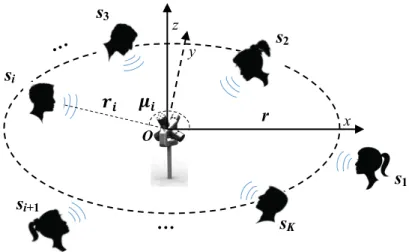
We suppose a scene where B-format microphone is located in the center of the room, as shown in Figure1. There exist a certain number of speakers in the horizontal plane of the microphone with different angles relative to the center of the B-format microphone [22], i.e., pointO. In the discrete TF domain, the pressure signal recorded in free-field bychchannel can be written as:
Sch(n,l) = K
∑
i=1
Hch,i(n,l)·Si(n,l) (1)
whereSchrepresents one of the four recording signals by the B-format microphone (i.e.,sFLU,sFRD,
sBLD,sBRU).Siis one of theKsources with an orientation pair (ri,µi), where radiusriis the distance of
sourceiwith respect toO, andµiis the azimuth of sourceiwith respect to x-axis.nandlrepresent the
frame number and the frequency index, respectively.Hch,iis the transfer function from theithsource to
channelchof B-format microphone. Assuming the free-field model, the recording signalsS
{Sch}can
be transformed to the B-format, which consists of one omnidirectional (W) and three figure-of-eight directional (X, Y, Z) channels, i.e.,SW,SX,SY,SZ.
z
s
i y%
&%
'(
'(
&⊕
⊕
%
*
&, %
*
'(
*
&, (
*
',
',
&r
s
1s
2s
3…
s
i+1s
K-
.$
. x OFigure 1.Illustration of the multi-source model and configuration of recording scene. The surrounding sources are numberedS1toSK.
2.2. Limitation of the W-DO Assumption
W-disjoint orthogonality (W-DO) [23] reveals the sparsity speech sources, which means that only one source is active at a certain TF bin. Besides, the spatial information of sourceSis preserved in the B-format signal by [24,25]: SW(n,l) = √ 2 2 ·S(n,l) SX(n,l) =cosµ·cosη·S(n,l) SY(n,l) =sinµ·cosη·S(n,l) SZ(n,l) =sinη·S(n,l) (2)
whereSis the sound source signal, andµandηare the azimuth and elevation of the sound source,
respectively, with respect to the center point O. If the W-DO property is valid, similar to [21], the estimated DOA ˆµ(n,l)of each TF bin can be obtained by:
ˆ
µ(n,l) =arctanIY(n,l)
IX(n,l)
(3) whereIYandIXcan be calculated by:
(
IX(n,l) =Re{S∗W(n,l)·SX(n,l)}
IY(n,l) =Re{S∗W(n,l)·SY(n,l)}
(4)
whereRe{·}denotes taking a real part of the argument and∗denotes conjugation operation.
However, simultaneously occurring speech signals are more likely to overlap in the TF domain, which means that more than one source is active at a TF bin with certain probability [21]. Hence, if the overlapped TF bins of multiple sources occupy a excessive proportion, the localization of multiple sources will be badly influenced. Further, the source separation method based on the localization procedure is not valid again. To solve this problem, some efficient localization methods have been proposed based on single-source bins or zone detection [26]. However, these methods can not eliminate the aliasing of TF components of the multiple source signals. As a result, the aliasing of the TF components cannot be recovered completely, which leads to poor separation quality in the case of the multiple sources. These overlapped TF components are defined as non-sparse components (which cause the famous cocktail problem), while the other TF components derived from one source are defined as sparse components.
In order to verify the W-DO assumption has reduced accuracy with an increasing number of simultaneously occurring sources, we examine how many TF bins are overlapped in the TF domain.
The ratio of overlapped TF bins (ROTF) can be defined as the measure to detect the proportion of non-sparse components, i.e.,
ROTF=1− K1 K
∑
i=1 1 N N∑
n=1 ||S0i(n,l)||0 ||Si(n,l)||0 ! (5)whereNis the number of total frames and quasi-norm|| · ||0counts the number of non-zero components
in its argument.S0i(n,l)can be obtained by:
S0i(n,l) = Si(n,l),i f|Si(n,l)| K ∑ j=1 Sj(n,l) >ξ,l ∈[1,L] 0,else (6)
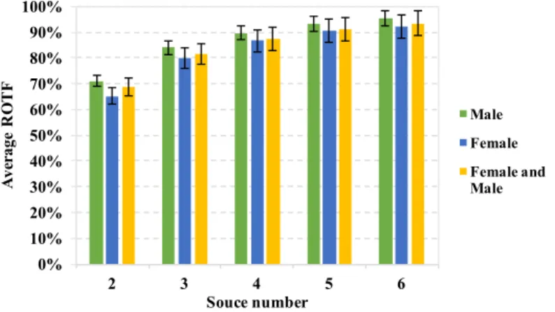
whereLis the number of STFT points in a frame. We detect the TF instant where only one source of energy is dominant among all sources, and then calculate the proportion of the these instants. Eventually, the ROTF is defined by subtracting the proportion. The ROTF implies the ratio of overlapped components amongKsimultaneously occurring sources. Obviously, a higher ROTF means weaker sparsity among these sources.
In order to examine the average ROTF among simultaneously occurring speech signals, statistical analysis is performed. In total, 36 sentences (the sampling frequency is 16 kHz) from the NTT [27] speech database are used for testing. In the following evaluation, all the test data is from the NTT [27] database unless otherwise stated. Each sentence was divided into a group with the otherK−1
(2≤K≤6)sentences in the time domain, resulting inKsimultaneously occurring speech conditions. ForK= 2, each sentence was divided into a group with each of the remaining 35 sentences resulting 36×35 = 1260 combinations. ForK > 2, each sentence was randomly grouped 35 times withK−1 other sentences to give the same number of combinations (1260) as forK= 2. In addition,ξ = 0.9.
The average length of each recording is about 8 s. Based on the aforementioned conditions, a statistical analysis of ROTF is taken. Statistical results are shown in Figure2with 95% confidence intervals.
0% 10% 20% 30% 40% 50% 60% 70% 80% 90% 100% 2 3 4 5 6 A ve rage RO T F Souce number Male Female Female and Male
Figure 2.Average ratio of overlapped time-frequency (ROTF) for 2–6 sources.
It can be observed that more TF bins are overlapped when the number of simultaneously occurring sources is increasing. In particular, whenK ≥ 5, the TF bins are almost overlapped, with a high percentage of over 90%.
3. Proposed Method
Based on the investigation in Section2, we can conclude that the W-DO has less accuracy as the number of simultaneously occurring sources increases. In order to eliminate the problem of poor
separation quality caused by this phenomenon, we propose a multiple source separation method based on self-reduction of dimensionality by using a B-format microphone. After proposing an effective detection method of the active sources in a non-sparse bin, we conduct a statistical analysis on the active source number that is involved in the non-sparse components and the corresponding possibility. It is found that when there exist Ksound sources simultaneously and the non-sparse components are mostly caused by less thanK/2 sound sources, it is very rare that the TF components of all sound sources are overlapped. Therefore, based on this phenomenon, we assume that when Ksound sources simultaneously occur in a sound scene, the active source number corresponding to the non-sparse component does not exceedK/2, which we call the half-K assumption. In addition, due to the recording characteristics of B-format microphone, we can get three linear equations with K source signals as independent variables. If the number of sound sources is greater than three, the linear equations will have multiple solutions, so the B-format microphone can only be used to separate the source signals of the scene with three sound sources. Based on the half-K assumption proposed in this paper, the B-format microphone can be used to solve the separation problem in the sound scene with six sound sources.
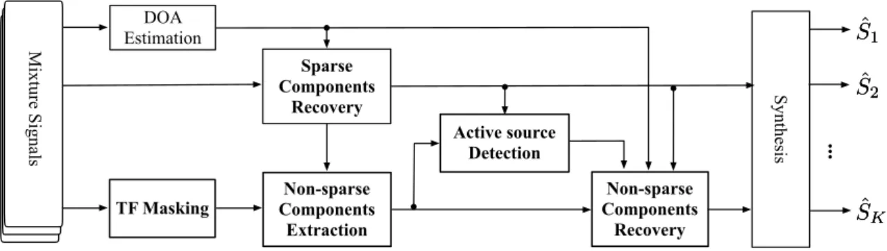
The illustration of the proposed BSS scheme is shown in Figure3. For the input mixture signals (four recording signals of the B-format microphone [21]), the DOA estimation can be obtained by a traditional localization procedure [21]. Thereafter, the sparse components recovery can be achieved by a clustering process of TF bins. The unprocessed non-sparse components are then obtained by masking the recovered sparse components from mixture signals. The half-K assumption provides a reduction of the dimensionality of the linear equations. By solving the linear equations, the non-sparse components will be effectively separated. Eventually, the final TF coefficients of each source will be recovered by the synthesis of sparse and non-sparse components.
M ixt ure S igna ls Sparse Components Recovery
TF Masking Components Non-sparse
Recovery S ynt he sis ... DOA Estimation Non-sparse Components Extraction Active source Detection
ˆ
S
ˆ
1S
1ˆ
S
ˆ
2S
2ˆ
S
ˆ
KS
K Figure 3.System block diagram of the proposed method. DOA: direction of arrival; TF: time-frequency.3.1. Separation of Sparse Components
Under the sparse assumption discussed in [20], one source will have the same mixing parameter pairsAandµ. For a given TF instant ofithsource, this pair is approximated by:
[Ai(n,l),µ(n,l)] = IY(n,l) IX(n,l) ,∠ IY(n,l) IX(n,l) (7) The separated sources can be derived by grouping the TF instants using these parameter pairs. If the estimated DOA of ith source is µi, the task is to determine a range around µi
(i.e., [µi−∆µ,µi+∆µ]) such that the TF instants having the DOA estimates within this range are
considered as the sourcei. It should be noted that if the threshold is set small enough, less interference from other sources may be contained in the separation. However, this may fail to derive many TF components whose DOA estimates are slightly different to the true source DOA due to the low fault tolerance of the estimation approach. If the threshold is larger, this may lead to the inclusion in the
separated source of TF components from other sources. Hence, an efficient clustering method is needed to dynamically achieve the separation of sparse components.
Based on the directional characteristic of B-format microphone, it can be seen that a strong correlation between the recording signals of adjacent channels in a certain TF zone implies that there is only one source active, while a weaker correlation means it is a region where multiple sources exist [21]. Hence, in this paper, we proposed a dynamic threshold clustering method of sparse components based on the inter-correlation of the raw recording (A-format) signals [21], and the threshold∆µis
dynamically set by:
∆µ= 1
1+e−α(γ−β)·µ0 (8)
whereµ0,α, andβare initial thresholds for the user to define;µ0is the threshold to control the dynamic
range of the∆µ,αis a threshold for controlling the∆µchange curve, and βis a symmetric point
corresponding to the change curve. ¯γis the average of normalized cross-correlation coefficients [21]
among four recording signals of the B-format microphone. More specifically, for any pair of soundfield microphone-recorded signals (Schi(n,l)andSchj(n,l)), the function is defined as:
Ri,j(K) =
∑
(n,l)∈K
|Schi(n,l)·Schj(n,l)| (9)
where i 6= j, Schi(n,l),Schj(n,l) ∈ {Sch1(n,l),Sch2(n,l),Sch3(n,l),Sch4(n,l),}. The normalized
cross-correlation coefficient can be obtained by:
γi,j(K) =
Ri,j(K) q
Ri,i(K)·Rj,j(K)
(10)
It can be seen from Equation (8) that the value of∆µis proportional to the correlation coefficient.
Specifically, if the correlation coefficient is close to one, the threshold will be large to obtain more extractions of the corresponding source, while in other TF zones, it will get smaller with the average correlation coefficient being smaller in order to get rid of the interference of other sources. Considering this issue and the value range of the cross-correlation coefficient, Equation (8) should be a function whose independent and dependent variables are both with a value range in [0, 1]. By adjusting the value of αand β, we find α = 10 and β = 0.5 can perfectly meet the requirement
mentioned above. Future work will investigate alternative methods for optimizing the choice of these values and find whether there might be a more efficient function that can describe the relation between
γand∆µ.
To make full use of the directional characteristic of B-format microphone, we can obtain the most appropriate vector as the mixed signal for source separation which can be obtained bySX andSY.
It was found experimentally that the performance degrades when processing ofSWis employed for
source separation, and a similar phenomenon was also found in other work [28]. In detail, the most appropriate vector[f1,f2, ...,fK]TofKsources can be obtained by:
f1 f2 .. . fK = cosµ1 cosµ2 sinµ1 sinµ2 .. . cosµK .. . sinµK " SX SY # (11)
Algorithm 1Sparse Component Separation Input:[f1,f2, ...,fK].
Initialize:Divide the frame intoJ sub-band regions with a equal width in the TF domain. forl=0, 1, ...,Ldo
Calculate the average of normalized cross-correlation ¯γ, and obtain the∆µby Equation (8).
Obtain the sparse components SCi of source i by clustering the TF components by parameter pair {fi,µi}.
end for
Output: Eventually, we will get the sparse componentsSCi of each source. 3.2. Exploring Inter-Sparsity among Multiple Sources
Further, in order to investigate the inter-sparsity among multiple sources, and how many active sources are involved in the overlapped TF bins, we proposed a statistic algorithm of the number of the active source at each TF instant when there occur multiple sources. In detail, the source whose energy at a certain TF instant is dominant among all the sources is regarded as the active source at this instant, i.e., its energy occupies a significant proportion of the total energy of all sources. To find the proportion of active source number when different numbers of sources occur, we define a statistical measure which is reflected in Algorithm2.
Algorithm 2Statistic of Active Source Number
Input:Sna = (ali)L×K= [S1nSn2 · · · SnK], whereSni = [|Si(n, 1)|,|Si(n, 2)|, ...,|Si(n,L)|]T.
Initialize:Counter= [Count1,Count2, ...,CountK] =0,cis used for counting the active source number
within current TF bin,c=0, loop frequency index:l= 1, loop source index:i= 0. forl=1, ...,Ldo fori=1, ...,Kdo ifali>η· K ∑ j=1| Sj(n,l)| incrementc. end if end for
incrementCounterc(i.e., increment value of the element incounterwhose index isc).
Reset:c=0. end for
Output:Counter.
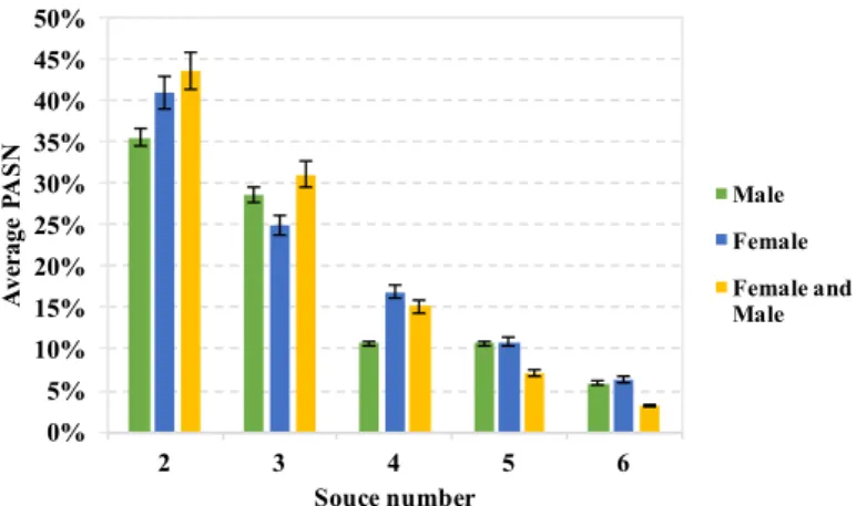
Then, we can calculate the probability of active source number (PASN) amongKsimultaneously occurring sources as:
PASN(c) = Counterc
L (12)
whereCountercdenotes the number of TF instants whencsources are active simultaneously,Lis the
number of STFT points in a frame, andPASN(c)represents the probability of TF bins which contain cactive sources. In other words, it implies the probability ofcsources active simultaneously over all TF bins. In order to analyze thePASNamongKsimultaneously occurring sources, we calculate thePASNof all groups mentioned above whenK=6. The results are shown in Figure4with 95% confidence intervals.
It can be seen that when there are six simultaneously occurring speech sources, most of the time only two or three sound sources are active at the same time over the non-sparse TF bins (occupying nearly 70%), i.e., most of the non-sparse components are involved with two or three sources. This implies that the proposed half-K assumption that no more thanK/2 sources are active in a certain TF bin when there areKsimultaneously occurring speech sources is reasonable.
0% 5% 10% 15% 20% 25% 30% 35% 40% 45% 50% 2 3 4 5 6 A ve rage PA S N Souce number Male Female Female and Male
Figure 4.Average probability of active source number (PASN) among six simultaneously occurring sources.
3.3. Separation of Non-Sparse Components
Based on the statistical results in Section3.2, we have validated the half-K assumption that the active source number in a certain TF bin does not exceed half the total number of simultaneously occurring sources. It means that forKsources, there are no more thanK/2 sources active at a certain TF bin. We set K ≤ 6 to ensure the localization accuracy in this work. Based on the proposed assumption, we can conclude that the number of active sources at a certain TF bin (Ka) is no more than
three. It should be noted thatKa =1 means that there is only one source active at a certain TF bin,
i.e., the sparse bin. The set of these sparse bins are the above-mentioned sparse components.
Aiming to separate the corresponding non-sparse components of each source, we have to know all the active sources of the non-sparse components. Here, the problem is solved by first dividing the TF band into several zones with same width, and then calculating the similarity between the separated sparse components and the mixture signal in this TF zone. In detail, if the similarity exceeds a certain threshold, the frequency components of the regions are mostly derived from this source signal and the signal set that satisfies the threshold is named the active source in the current TF zone of non-sparse components. The normalized cross-correlation function is utilized for similarity calculation, and the cross-correlation coefficient between the mixture signalSWand a sparse component signalSiCin a TF
zoneZ is calculated as follows:
RS W,SCi (Z) = ∑ (n,l)∈Z| SW(n,l)| · |SCi (n,l)| r ∑ (n,l)∈Z| SW(n,l)|2· ∑ (n,l)∈Z| SCi (n,l)|2 (13) whereSC
i represents the separated sparse component signal and i = 1, 2, ...,K. To obtain all the
active sources of non-sparse components in a TF-analyzed oneZ, we define a active detecting vector D= [D1,D2, ...,DK]; theith elementDican be obtained by:
Di = (
1, ifRSW,SCi(Z)>e
0,else (14)
whereeis an experimental threshold, in order to ensure that the number detected active sound source
is not larger than the real one. We sete=0.8 in this paper (informal testing found this value generally
led to satisfactory results but future work can explore the optimization of this value). The index value of the detected active source is recorded in a vectorI, which can be obtained by aI NDEX0function as:
I= I NDEX0(D) (15) whereI NDEX0(·)is a non-zero index searching function; the output parameter is a vector that contains
all the indexes of non-zero elements of the input vector.
||D||0=3, i.e.,I = [I1,I2,I3], where|| · ||0counts the number of non-zero components in its
argument. This means there are three active sources at the current zone. Hence, the corresponding TF coefficient of these active sources is rewritten to find a solution to the linear equations:
√ 2 2 √ 2 2 √ 2 2
cosµI1 cosµI2 cosµI3
sinµI1 sinµI2 sinµI3
SI1(n,l) SI2(n,l) SI3(n,l) = SW(n,l) SX(n,l) SY(n,l) (16)
whereµI1,µI2,µI3 denote the estimated DOA of the active source by applying the method in [21].
Equation (16) can be rewritten as a vector form as:
KSI =S (17)
whereSI = [SI1(n,l),SI2(n,l),SI3(n,l)]
T andS= [S
W(n,l),SX(n,l),SY(n,l)]T.The separation problem
is converted to solve the linear equations by regarding the TF coefficient of each active source as an independent variable. It should be mentioned that the process is based on the hypothesis that the mixing matrix of Equation (16) is a column full rank matrix. To jointly consider the case||D||0>3,
the aim is converted to find a vectorSN
I = [SIN1(n,l),SIN2(n,l),SNI3(n,l)]to minimize||S−KSI||2F, i.e.,
SIN=arg min
SI ||
S−KSI||2F (18)
where|| · ||Frepresents the Frobenius norm.SINrepresents the separated TF coefficients of the active
sources at(n,l).
For the case||D||0=2, i.e.,I = [I1,I2], we can omit the first equation in Equation (16) i.e.,
" cosµI1 cosµI2 sinµI1 sinµI2 # " SI1(n,l) SI2(n,l) # = " SX(n,l) SY(n,l) # (19) We can still get the solution by solving Equation (18) for this case. Then, we can get the actual TF coefficients ofSI1(n,l)andSI2(n,l)by:
SIN 1(n,l) = sin(µI2)·SX(n,l)−cos(µI2)·SY(n,l) sin(µI2−µI1) SIN 2(n,l) = sin(µI1)·SX(n,l)−cos(µI1)·SY(n,l) sin(µI1−µI2) (20)
Finally, the final recovered signal can be obtained by a synthesis as: ˆ
Si(n,l) =SCi (n,l) +SiN(n,l) (21)
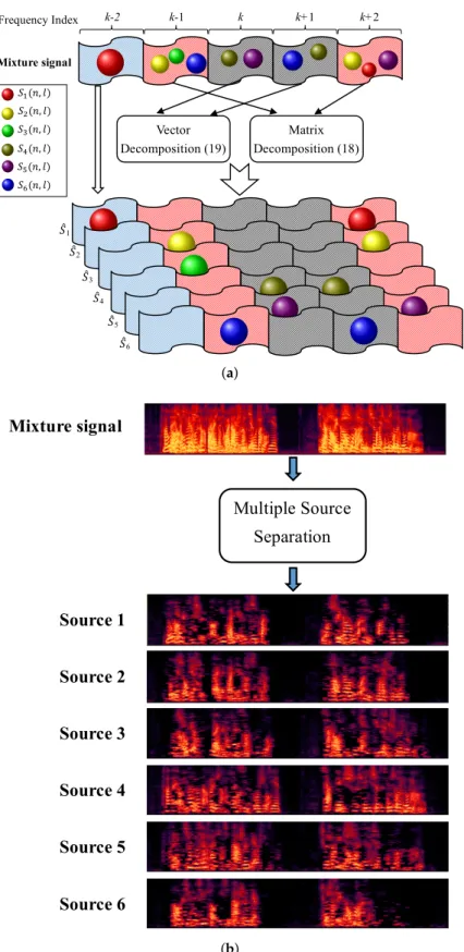
Figure5a illustrates an example of the TF component extraction of the proposed method. Figure5b is an example of the recovered signals from the mixture signal.
Appl. Sci. 2018,8, 123 11 of 23 Multiple Source Separation Mixture signal Source 1 Source 2 Source 3 Source 4 Source 5 Source 6 !"1 !"2 !"3 !"4 !"5 !"6 1 2 3 4 5 0.2 0.4 0.6 Harmonic order Ma g n it u d e 5 1 2 3 4 5 0.2 0.4 0.6 Harmonic order Ma g n it u d e 5 1 2 3 4 5 0.2 0.4 0.6 Harmonic order Ma g n it u d e 5 1 2 3 4 5 0.2 0.4 0.6 Harmonic order Ma g n it u d e 5 1 2 3 4 5 0.2 0.4 0.6 Harmonic order Ma g n it u d e 5 1 2 3 4 5 0.2 0.4 0.6 Harmonic order Ma g n it u d e 5 1 2 3 4 5 0.2 0.4 0.6 Harmonic order Ma g n it u d e 5 1 2 3 4 5 0.2 0.4 0.6 Harmonic order Ma g n it u d e 5 1 2 3 4 5 0.2 0.4 0.6 Harmonic order Ma g n it u d e 5 1 2 3 4 5 0.2 0.4 0.6 Harmonic order Ma g n it u d e 5 1 2 3 4 5 0.2 0.4 0.6 Harmonic order Ma g n it u d e 5 1 2 3 4 5 0.2 0.4 0.6 Harmonic order Ma g n it u d e 5 1 2 3 4 5 0.2 0.4 0.6 Harmonic order Ma g n it u d e 5 1 2 3 4 5 0.2 0.4 0.6 Harmonic order Ma g n it u d e 5 1 2 3 4 5 0.2 0.4 0.6 Harmonic order Ma g n it u d e 5 1 2 3 4 5 0.2 0.4 0.6 Harmonic order Ma g n it u d e 5 1 2 3 4 5 0.2 0.4 0.6 Harmonic order Ma g n it u d e 5 !#(%, ') !)(%, ') !*(%, ') !+(%, ') !,(%, ') !-(%, ') Frequency Index Vector Decomposition (19) 1 2 3 4 5 0.2 0.4 0.6 Harmonic order Ma g n it u d e 5 1 2 3 4 5 0.2 0.4 0.6 Harmonic order Ma g n it u d e 5 1 2 3 4 5 0.2 0.4 0.6 Harmonic order Ma g n it u d e 5 1 2 3 4 5 0.2 0.4 0.6 Harmonic order Ma g n it u d e 5 1 2 3 4 5 0.2 0.4 0.6 Harmonic order Ma g n it u d e 5 1 2 3 4 5 0.2 0.4 0.6 Harmonic order Ma g n it u d e 5 1 2 3 4 5 0.2 0.4 0.6 Harmonic order Ma g n it u d e 5 1 2 3 4 5 0.2 0.4 0.6 Harmonic order Ma g n it u d e 5 1 2 3 4 5 0.2 0.4 0.6 Harmonic order Ma g n it u d e 5 1 2 3 4 5 0.2 0.4 0.6 Harmonic order Ma g n it u d e 5 1 2 3 4 5 0.2 0.4 0.6 Harmonic order Ma g n it u d e 5 Mixture signal k+1 k-1 k k-2 k+2 Matrix Decomposition (18) (a)
Multiple Source
Separation
Mixture signal
Source 1
Source 2
Source 3
Source 4
Source 5
Source 6
!"1
!"
2!"
3!"4
!"5
!"
6 1 2 3 4 5 0.2 0.4 0.6 Harmonic order Ma g n it u d e 5 1 2 3 4 5 0.2 0.4 0.6 Harmonic order Ma g n it u d e 5 1 2 3 4 5 0.2 0.4 0.6 Harmonic order Ma g n it u d e 51
2
3
4
5
0
.
2
0
.
4
0
.
6
Harmonic order Ma g n it u d e5
1 2 3 4 5 0.2 0.4 0.6 Harmonic order Ma g n it u d e 5 1 2 3 4 5 0.2 0.4 0.6 Harmonic order Ma g n it u d e 5 1 2 3 4 5 0.2 0.4 0.6 Harmonic order Ma g n it u d e 5 1 2 3 4 5 0.2 0.4 0.6 Harmonic order Ma g n it u d e 5 1 2 3 4 5 0.2 0.4 0.6 Harmonic order Ma g n it u d e 5 1 2 3 4 5 0.2 0.4 0.6 Harmonic order Ma g n it u d e 5 1 2 3 4 5 0.2 0.4 0.6 Harmonic order Ma g n it u d e 5 1 2 3 4 5 0.2 0.4 0.6 Harmonic order Ma g n it u d e 5 1 2 3 4 5 0.2 0.4 0.6 Harmonic order Ma g n it u d e 5 1 2 3 4 5 0.2 0.4 0.6 Harmonic order Ma g n it u d e 5 1 2 3 4 5 0.2 0.4 0.6 Harmonic order Ma g n it u d e 5 1 2 3 4 5 0.2 0.4 0.6 Harmonic order Ma g n it u d e 5 1 2 3 4 5 0.2 0.4 0.6 Harmonic order Ma g n it u d e 5 !#(%, ') !)(%, ') !*(%, ') !+(%, ') !,(%, ') !-(%, ')Vector
Decomposition (17)
1
2
3
4
5
0
.
2
0
.
4
0
.
6
Harmonic order Ma g n it u d e5
1
2
3
4
5
0
.
2
0
.
4
0
.
6
Harmonic order Ma g n it u d e5
1
2
3
4
5
0
.
2
0
.
4
0
.
6
Harmonic order Ma g n it u d e5
1
2
3
4
5
0
.
2
0
.
4
0
.
6
Harmonic order Ma g n it u d e5
1
2
3
4
5
0
.
2
0
.
4
0
.
6
Harmonic order Ma g n it u d e5
1
2
3
4
5
0
.
2
0
.
4
0
.
6
Harmonic order Ma g n it u d e5
1
2
3
4
5
0
.
2
0
.
4
0
.
6
Harmonic order Ma g n it u d e5
1
2
3
4
5
0
.
2
0
.
4
0
.
6
Harmonic order Ma g n it u d e5
1
2
3
4
5
0
.
2
0
.
4
0
.
6
Harmonic order Ma g n it u d e5
1
2
3
4
5
0
.
2
0
.
4
0
.
6
Harmonic order Ma g n it u d e5
1
2
3
4
5
0
.
2
0
.
4
0
.
6
Harmonic order Ma g n it u d e5
Mixture signal
Matrix
Decomposition (16)
(b)Figure 5.(a) Example of a TF component extraction of the proposed framework. Both the frame length and number of STFT points are 2048. Each square represents a TF instant. Blue-shadowed squares denote the sparse component, while the squares in other colors denote the non-sparse component. The respective TF instants for each source (six sources for example) are indicated by a ball; (b) Example of six recovered signals from the mixture signal in the frequency domain.
4. Evaluation
In this section, to verify the effectiveness of the proposed method, a series of objective and subjective evaluation tests are presented. Several aspects are considered in the tests to assess the separation quality including source number, the angle between sources, and the environment.
NTT [27], as a speech database including various speakers from different countries, has been chosen as the testing database. In addition, all the data are monorecordings and the energy of all speech in NTT database is the same. Thus, this database is suitable for evaluating the quality of multiple speech object separation methods. For the evaluation in simulated scenarios, all of the test segments are derived from the database. Each test segment representing a speech source is created with a length of 8 s. In order to evaluate the separation quality when different types of multiple speech sources are active simultaneously, a complicated situation where different proportions of male and female speakers are simultaneously talking is considered in this work.
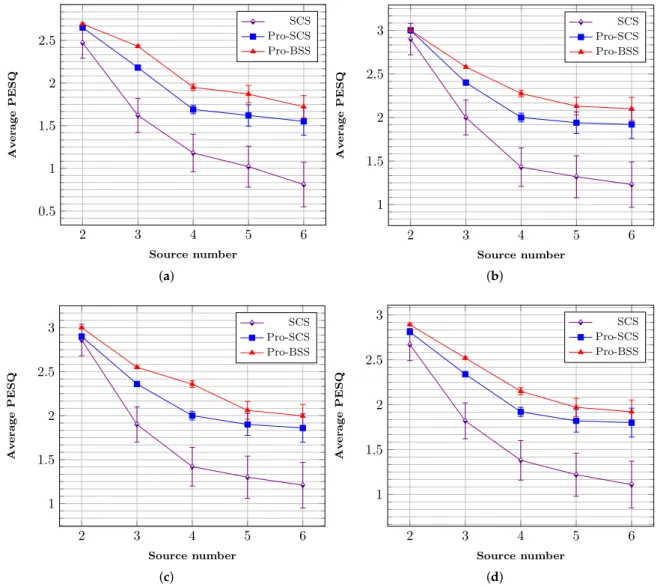
To evaluate the proposed method in different environments, we used Roomsim [29] to simulate a room measuring 6.25×4.75×2.5 m3with different reverberation conditions. The main parameters of
the simulated rooms are illustrated in Table 1. The B-format microphone was placed in the center of the room parallel with thez-axis, and the power of sound sources from different directions was equal in each simulation. It should be noted that the B-format microphone was simulated via Roomsim, and was completed by simulating the recording condition of each channel. In addition, the radius of the cube (radius of the circumscribed circle) is 12 mm. The azimuth and elevation pairs of the four channels (i.e., FLU, FRD, BLD, and BRU) are{(45◦, 45◦),(−45◦,−45◦),(135◦,−45◦),(−135◦, 45◦)}. For the objective evaluation in real environments, all the test data was recorded in a room measuring 6.25×4.75×2.5 m3,SNR= 20 dB,RT60 = 0.5 s.
In addition, the width of TF-analyzed region mentioned in Section 2 is determined by applications. In this work, in order to obtain a most efficient width of the TF-analyzed zone, we took a number of tests and found that the score keeps stable for five different widths:{128, 64, 32, and 16}. We chose 64 as the width in [21] for “single-source” zone detecting, so the width of analyzed TF zone was also set by a constant of 64 considering both efficiency and low computational complexity. Other allocation strategies might improve the quality of individual speech sources or balance the quality amongst all sources, which will be investigated as the future work.
Table 1.Parameters of the testing room.
Simulated Room Absorption of the Wall RT60(ms) Reflection Order
Anechoic Room 1 0 0
Room1 0.75 250 18
Room2 0.75 500 18
4.1. Objective Evaluation
For objective evaluation, three measurements, i.e., perceptual evaluation of speech quality (PESQ) [30], signal-to-distortion ratio (SDR) and signal-to-interference ratio (SIR) were adopted to evaluate the perceptual quality of extracted speech signals. Specifically, the PESQ generated by the evaluation software [30] was used to evaluate the perceptual similarity between the separated signal and the original signal. The score interval of PESQ is[0, 5], where smaller values imply a degradation of the quality of separated speech signal. The SDR and SIR were obtained by using the BSS EVAL Toolbox [31]; the SDR measures the overall performance (quality) of the algorithm, and the SIR focuses on the interference rejection. The tests were conducted in both simulated scenarios and real environments.
For comparison, one of the most efficient sparse component separation (SCS) methods was selected as the reference method [28] to indicate the effect of the non-sparse component recovery by using the proposed method. Then, five outstanding existing methods were chosen for further evaluation.
Specifically, for the determined case (K=3 in this paper), we compared the PESQ score of our proposed method with BSS methods, which belongs to other categories under simulated condition.
4.1.1. Simulated Environment
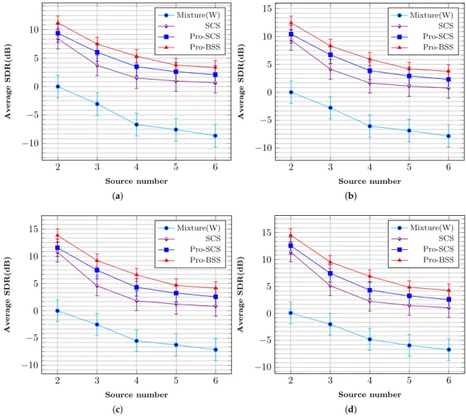
First, by evaluating the same test data in s environment, the average PESQ scores of fixed threshold method and our proposed approach virus different source numbers and separations are shown in Figure6. Condition SCS is the result extracted by the fixed threshold (i.e.,∆µ = µ0 = 8◦) sparse
component separation method, while Pro-SCS is the proposed approach of sparse components with a dynamic threshold, and condition Pro-BSS is the proposed sparse and non-sparse component separation method. Figure6a–d represents the result for separations {30◦, 40◦, 50◦, 60◦}. It can be seen that the two proposed separation methods reach a higher score, especially forsource number>3. In addition, Pro-BSS reaches the highest score, and the average scores are all above 2 for all source numbers, which indicates a better perceptual quality of the proposed method compared to the fixed threshold separation approach.
2 3 4 5 6 1 1.5 2 2.5 3 Source number Av erage PE SQ SCS Pro-SCS Pro-BSS 2 3 4 5 6 0.5 1 1.5 2 2.5 Source number Av erage PE SQ SCS Pro-SCS Pro-BSS 2 (a) 2 3 4 5 6 1 1.5 2 2.5 3 Source number Av erage PE SQ SCS Pro-SCS Pro-BSS 2 3 4 5 6 1 1.5 2 2.5 3 Source number Av erage PE SQ SCS Pro-SCS Pro-BSS 1 (b) 2 3 4 5 6 1 1.5 2 2.5 3 Source number Av erage PE SQ SCS Pro-SCS Pro-BSS 2 3 4 5 6 1 1.5 2 2.5 3 Source number Av erage PE SQ SCS Pro-SCS Pro-BSS 1 (c) 2 3 4 5 6 1 1.5 2 2.5 3 Source number Av erage PE SQ SCS Pro-SCS Pro-BSS 2 3 4 5 6 0 2 4 6 Source number MA E E (d e g r e e s) Separation=30 Separation=40 Separation=50 Separation=60 2 (d)
Figure 6.Perceptual evaluation of speech quality (PESQ) results. Error bars represent 95% confidence intervals; (a–d) represent the results for separations {30◦, 40◦, 50◦, 60◦}. SCS: sparse component separation; Pro-SCS: the proposed approach of sparse components with a dynamic threshold; Pro-BSS: the proposed sparse and non-sparse component separation method.
Appl. Sci. 2018,8, 123 14 of 23
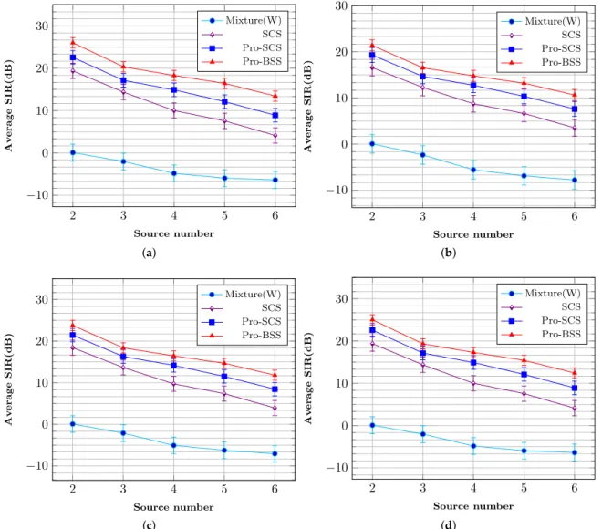
The corresponding results are shown in Figures7and8, respectively. Condition mixture (W) represents the B-format input signalSW. The SDR and SIR results follow a similar trend to the PESQ
results. Overall, it can be concluded that the proposed method obtains a great improvement in extracted sources. 2 3 4 5 6 10 5 0 5 10 Source number Av erage SDR(dB) Mixture(W) SCS Pro-SCS Pro-BSS 2 3 4 5 6 10 5 0 5 10 15 Source number Av erage SDR(dB) Mixture(W) SCS Pro-SCS Pro-BSS (a) 2 3 4 5 6 10 5 0 5 Source number Av erage SDR(dB) Pro-SCS Pro-BSS 2 3 4 5 6 10 5 0 5 10 15 Source number Av erage SDR(dB) Mixture(W) SCS Pro-SCS Pro-BSS (b) 2 3 4 5 6 10 5 0 5 10 15 Source number Av erage SDR(dB) Mixture(W) SCS Pro-SCS Pro-BSS 2 3 4 5 6 10 5 0 5 10 15 Source number Av erage SDR(dB) Mixture(W) SCS Pro-SCS Pro-BSS (c) 2 3 4 5 6 10 5 0 5 10 15 Source number Av erage SDR(dB) Mixture(W) SCS Pro-SCS Pro-BSS 2 3 4 5 6 10 5 0 5 10 15 Source number Av erage SDR(dB) Mixture(W) SCS Pro-SCS Pro-BSS (d)
Figure 7. Signal-to-distortion ratio (SDR) results. Error bars represent 95% confidence intervals; (a–d) represent the results for separations {30◦, 40◦, 50◦, 60◦}.
Eventually, for the determined case (i.e.,K = 3), we conducted a comparison with four other existing approaches: (a) spatio-temporal ICA [32] applied using a single (recording fromMi using
channelWi,Xi,Yi) B-format speech mixture (S-ICA); (b) spatio-temporal ICA applied using a dual
(recording from Mi using channelWi, Xi,Yi and corresponding channels of Mj) B-format speech
mixture (D-ICA); (c) source DOA-based BSS using single coincident microphone recording (S-BSS) [28]; and DOA-based collaborative BSS (CBSS) [20] using a pair of coincident spatial microphones. Note that the reference mixture (W) is an unprocessed speech mixture (W channel of the B-format recording) used for indicating the worst quality. It should be noted that there are still many good algorithms, like the independent vector analysis (IVA)-based method [33,34], the independent low-rank matrix analysis (ILRMA)-based method, and so on [35]. Their methods focus on audio source separation, while we prefer the case with all speech sources, so only a few algorithms are chosen for comparison.
Appl. Sci. 2018,8, 123 15 of 23 2 3 4 5 6 10 0 10 20 30 Source number A v e r a g e S IR (d B ) Mixture(W) SCS Pro-SCS Pro-BSS 2 3 4 5 6 10 0 10 20 30 Source number A v e r a g e S IR (d B ) Mixture(W) SCS Pro-SCS Pro-BSS (a) 2 3 4 5 6 10 0 10 20 Source number A v e r a g e S IR (d B ) SCS Pro-SCS Pro-BSS 2 3 4 5 6 10 0 10 20 30 Source number A v e r a g e S IR (d B ) Mixture(W) SCS Pro-SCS Pro-BSS (b) 2 3 4 5 6 10 0 10 20 30 Source number A v e r a g e S IR (d B ) Mixture(W) SCS Pro-SCS Pro-BSS 2 3 4 5 6 10 0 10 20 30 Source number A v e r a g e S IR (d B ) Mixture(W) SCS Pro-SCS Pro-BSS real (c) 2 3 4 5 6 10 0 10 20 30 Source number A v e r a g e S IR (d B ) Mixture(W) SCS Pro-SCS Pro-BSS 2 3 4 5 6 10 0 10 20 30 Source number A v e r a g e S IR (d B ) Mixture(W) SCS Pro-SCS Pro-BSS real (d)
Figure 8. Signal-to-interference ratio (SIR) results. Error bars represent 95% confidence intervals; (a–d) represent the results for separations {30◦, 40◦, 50◦, 60◦}.
From Figure9, the proposed BSS approach outperforms the other BSS techniques based on the PESQ measure. It should be noted that Figure9a–c are calculated by different references in order to compare the separated speech using different methods under the same acoustic condition. In detail, for the reverberant conditions, the reference is selected as the clean speech with the same level of reverberation rather than anechoic clean speech. The major improvement (approximately 1 against the third best) is achieved by the proposed dynamic threshold-based sparse components and stability-based non-sparse components separation. Specifically, compared with C-BSS, we achieve a better perceptual quality by using only a B-format microphone, while C-BSS adopts a pair.
4.1.2. Real Environment
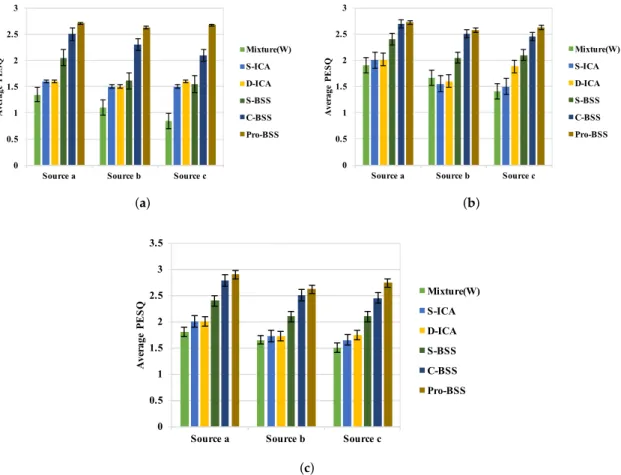
In total, 36 sentences (sampling frequency 16 kHz) recorded in a room measuring 10×5×3 m3 (SNR= 20 dB, RT60 = 0.5 s) were utilized for the evaluation in a real environment. The average length of each recording is also about 8 s same as NTT [27] database. Based on the aforementioned conditions, a statistical analysis ofPESQis taken. Statistical results are shown in Figure10with 95% confidence intervals.
0 0.5 1 1.5 2 2.5 3
Source a Source b Source c
A ve rage PE S Q Mixture(W) S-ICA D-ICA S-BSS C-BSS Pro-BSS (a) 0 0.5 1 1.5 2 2.5 3
Source a Source b Source c
A ve rage PE S Q Mixture(W) S-ICA D-ICA S-BSS C-BSS Pro-BSS (b) 0 0.5 1 1.5 2 2.5 3 3.5
Source a Source b Source c
A ve rage PE S Q Mixture(W) S-ICA D-ICA S-BSS C-BSS Pro-BSS (c)
Figure 9.PESQ results (a) Anechoic Room; (b) Room1; (c) Room2. Error bars represent 95% confidence intervals.
From Figure10, we can concluded that the proposed method greatly improved the perceptual quality of extracted sources. The corresponding SDR and SIR results are shown in Figures11and12, respectively. Condition mixture (W) represents the B-format input signalSW. Similar to the results
in the simulated environment, the SDR and SIR results follow a similar trend to the PESQ results. Overall, it can be concluded that the proposed method obtain a great improvement of extracted sources. 4.2. Subjective Evaluation
Subjective evaluation consists of two major listening tests. For all cases (the overdetermined case, determined case, and underdetermined case), the perceptual quality of speech sources generated in section IV-A-1 corresponds to the case whereK={2, 3, 4, 5, 6}. The separation is{30◦, 40◦, 50◦, 60◦}, and the source radius is 1 m. Note that each separated speech source is evaluated separately by using headphones for playback. A MUSHRA [36] listening test which contains 16 listeners is employed to measure the subjective perceptual quality with four conditions, namely, Ref, Pro-BSS, Pro-SCS, SCS, and Anchor. Condition Ref refers to the original speech sources in each test, which are also served as the hidden references of this MUSHRA test. Condition SCS, Pro-SCS, and Pro-BSS are the same as in the objective evaluation. Condition Anchor is the unprocessed (W channel of the B-format recording) mixed signal. In total, 16 listeners participated in the test.
Appl. Sci. 2018,8, 123 17 of 23 2 3 4 5 6 1 1.5 2 2.5 Source number Av erage PE SQ Pro-SCS Pro-BSS 2 3 4 5 6 0.5 1 1.5 2 2.5 Source number Av erage PE SQ SCS Pro-SCS Pro-BSS (a) 2 3 4 5 6 1 1.5 2 2.5 3 Source number Av erage PE SQ SCS Pro-SCS Pro-BSS 2 3 4 5 6 0.5 1 1.5 2 2.5 Source number Av erage PE SQ SCS Pro-SCS Pro-BSS (b) 2 3 4 5 6 1 1.5 2 2.5 3 Source number Av erage PE SQ SCS Pro-SCS Pro-BSS 2 3 4 5 6 1 1.5 2 2.5 3 Source number Av erage PE SQ SCS Pro-SCS Pro-BSS (c) 2 3 4 5 6 1 1.5 2 2.5 3 Source number Av erage PE SQ SCS Pro-SCS Pro-BSS 2 3 4 5 6 1 1.5 2 2.5 3 Source number Av erage PE SQ SCS Pro-SCS Pro-BSS (d)
Figure 10.PESQ results. Error bars represent 95% confidence intervals, (a–d) represent the results for separations {30◦, 40◦, 50◦, 60◦},SNR= 20 dB,RT60 = 0.5 s.
For each source number and separation, we calculated the average of all tested speeches and results are shown in Figures13–16. It can be observed that our proposed method achieves significantly higher scores compared to the fixed threshold BSS approach, which uses the same number of microphones as our proposed method. In addition, the PSM scores decreases as the source number increases from 2 to 6, and rises as the separation between the two adjacent sources gets larger. For the casesK= 2, 3, the scores are always about 0.8, which reaches a nearly excellent quality. For the undermined case, the MUSHRA scores are about 0.7 when the source number is four, while for the casesK= 5, 6, the quality of the extracted speech is below 0.6 but still over 0.4. This means that the extracted speech is not quite euphonious but can still represent clear and understandable speech.
To compare the extracted speech quality with the reference method in objective evaluation further, a MUSHRA test was also employed to measure the subjective quality of the separated speech. Six middle sources from each test group were selected for the listening test. Similarly, the unprocessed (W channel of the B-format recording) mixed signal was used as the anchor and the original speech was used as the hidden reference. Note that each separated speech source is evaluated separately by using loudspeakers for playback in the Anechoic Room, Room 1, and Room 2. Average MUSHRA scores are presented in Figure17.
Appl. Sci. 2018,8, 123 18 of 23 2 3 4 5 6 10 5 0 5 10 Source number Av erage SDR(dB) Mixture(W) SCS Pro-SCS Pro-BSS 2 3 4 5 6 10 5 0 5 10 Source number Av erage SDR(dB) Mixture(W) SCS Pro-SCS Pro-BSS (a) 2 3 4 5 6 10 5 0 5 Source number Av erage SDR(dB) Pro-SCS Pro-BSS 2 3 4 5 6 10 5 0 5 10 Source number Av erage SDR(dB) Mixture(W) SCS Pro-SCS Pro-BSS (b) 2 3 4 5 6 10 5 0 5 10 15 Source number Av erage SDR(dB) Mixture(W) SCS Pro-SCS Pro-BSS 2 3 4 5 6 10 5 0 5 10 15 Source number Av erage SDR(dB) Mixture(W) SCS Pro-SCS Pro-BSS (c) 2 3 4 5 6 10 5 0 5 10 15 Source number Av erage SDR(dB) Mixture(W) SCS Pro-SCS Pro-BSS 2 3 4 5 6 10 5 0 5 10 15 Source number Av erage SDR(dB) Mixture(W) SCS Pro-SCS Pro-BSS (d)
Figure 11.SDR results. Error bars represent 95% confidence intervals, (a–d) represent the results for separations {30◦, 40◦, 50◦, 60◦},SNR= 20 dB,RT60 = 0.5 s.
It can be seen that a significant improvement in the separation quality is achieved by applying the proposed scheme. The MUSHRA score for the proposed method is of nearly ‘excellent’ quality, the second best score is about ‘good’. It should be noted that we just use one B-format microphone, while C-BSS adopts a pair. The majority of listeners indicated that their choice for the closest match to the reference was based on files which contained the minimal amount of crosstalk and musical distortion. For other conditions, listeners reported that while the target speech is significantly separated from the mixture, there is audible crosstalk from other talkers with higher musical distortion.
Appl. Sci. 2018,8, 123 19 of 23 2 3 4 5 6 10 0 10 20 30 Source number A v e r a g e S IR (d B ) Mixture(W) SCS Pro-SCS Pro-BSS 2 3 4 5 6 10 0 10 20 30 Source number A v e r a g e S IR (d B ) Mixture(W) SCS Pro-SCS Pro-BSS (a) 2 3 4 5 6 10 0 10 20 Source number A v e r a g e S IR (d B ) SCS Pro-SCS Pro-BSS 2 3 4 5 6 10 0 10 20 30 Source number A v e r a g e S IR (d B ) Mixture(W) SCS Pro-SCS Pro-BSS (b) 2 3 4 5 6 10 0 10 20 30 Source number A v e r a g e S IR (d B ) Mixture(W) SCS Pro-SCS Pro-BSS 2 3 4 5 6 10 0 10 20 30 Source number A v e r a g e S IR (d B ) Mixture(W) SCS Pro-SCS Pro-BSS (c) 2 3 4 5 6 10 0 10 20 30 Source number A v e r a g e S IR (d B ) Mixture(W) SCS Pro-SCS Pro-BSS 2 3 4 5 6 10 0 10 20 30 Source number A v e r a g e S IR (d B ) Mixture(W) SCS Pro-SCS Pro-BSS (d)
Figure 12.SIR results. Error bars represent 95% confidence intervals, (a–d) represent the results for separations {30◦, 40◦, 50◦, 60◦},SNR= 20 dB,RT60 = 0.5 s. 0 20 40 60 80 100 0 1 2 3 4 5 Source number Hidden Ref Pro-BSS Pro-SCS SCS Anchor Excellent Good Fair Poor Bad 100 80 60 40 20 0 2 3 4 5 6
0 20 40 60 80 100 0 1 2 3 4 5 Source number SCS Pro-SCS Pro-BSS Hidden Ref Anchor Excellent Good Fair Poor Bad 100 80 60 40 20 0 2 3 4 5 6
Figure 14.MUSHRA test results ofseparation=40◦. Error bars with 95% confidence intervals.
0 20 40 60 80 100 0 1 2 3 4 5 Source number SCS Pro-SCS Pro-BSS Hidden Ref Anchor Excellent Good Fair Poor Bad 100 80 60 40 20 0 2 3 4 5 6
Figure 15.MUSHRA test results ofseparation=50◦. Error bars with 95% confidence intervals.
0 20 40 60 80 100 0 1 2 3 4 5 Source number SCS Pro-SCS Pro-BSS Hidden Ref Anchor Excellent Good Fair Poor Bad 100 80 60 40 20 0 2 3 4 5 6
0 20 40 60 80 100 0 1 2 3 HiddenRef Pro-BSS C-BSS S-BSS D-ICA S-ICA Anchor Excellent Good Fair Poor Bad 100 80 60 40 20 0
Anechic Room 1 Room 2
Figure 17.MUSHRA test results. Error bars with 95% confidence intervals. 5. Conclusions
A multiple speech source separation method using inter-channel correlation and the half-K assumption was proposed in this paper. To recover the sparse components, we proposed a dynamic threshold-based clustering algorithm where the threshold was determined by the inter-channel correlation among the recording signals of B-format microphone. Thereafter, a half-K assumption was proposed after conducting a statistical analysis of the number of the active source at each TF instant versus different number of sources. By applying this assumption, the non-sparse components were separated by regarding the extracted sparse components as a guide, jointly combined with vector decomposition and matrix factorization. Ultimately, the final TF coefficients of each source were recovered by the synthesis of sparse and non-sparse components. The approach has been evaluated via objective and subjective tests for both the anechoic and reverberant condition. Compared with the fixed threshold sparse components separation method, the proposed approach achieved significant improvement in the perceptual quality of separated sources. In addition, the comparison was also conducted with other BSS approaches. According to both objective and subjective evaluation, the proposed method achieved a better perceptual quality of separated sources than others.
Acknowledgments:This work has been supported by China Postdoctoral Science Foundation(2017M610731), the Project supported by Beijing Postdoctoral Research Foundation and “Ri xin” Training Programme Foundation for the Talents by Beijing University of Technology.
Author Contributions:Maoshen Jia and Jundai Sun contributed equally in conceiving the overall proposal, and critically reviewed and implemented the final revisions. Maoshen Jia and Jundai Sun supervised all aspects of this separation architecture, design and realization of the experiments, collection and analysis of the data, and writing of the manuscript. Xiguang Zheng critically reviewed and implemented the final revisions.
Conflicts of Interest:The authors declare no conflicts of interest. References
1. Zheng, X.Soundfield Navigation: Separation, Compression and Transmission, Doctoral Dissertation; University of Wollongong: Wollongong, Austral, 2013.
2. Asaei, A.; Taghizadeh, M.J.; Haghighatshoar, S.; Raj, B.; Bourlard, H.; Cevher, V. Binary Sparse Coding of Convolutive Mixtures for Sound Localization and Separation via Spatialization. IEEE Trans. Signal Process. 2016,64, 567–579.
3. Jia, M.; Yang, Z.; Bao, C.; Zheng, X.; Ritz, C. Encoding Multiple Audio Objects Using Intra-Object Sparsity.
IEEE/ACM Trans. Audio Speech Lang. Process.2015,23, 1082–1095.
4. Zheng, X.; Ritz, C.; Xi, J. Encoding and communicating navigable speech soundfields.Multimed. Tools Appl. 2016,75, 5183–5204.
5. Hilpert, J.; Disch, S. The MPEG Surround Audio Coding Standard [Standards in a Nutshell].IEEE Signal Process. Mag.2009,26, 148–152.
6. Bahdanau, D.; Chorowski, J.; Serdyuk, D.; Brakel, P.; Bengio, Y. End-to-end attention-based large vocabulary speech recognition. In Proceedings of the 2016 IEEE International Conference on Acoustics, Speech and Signal Processing (ICASSP), Shanghai, China, 20–25 March 2016; pp. 4945–4949.
7. Petridis, S.; Pantic, M. Deep complementary bottleneck features for visual speech recognition. In Proceedings of the 2016 IEEE International Conference on Acoustics, Speech and Signal Processing (ICASSP), Shanghai, China, 20–25 March 2016; pp. 2304–2308.
8. Abou-Zleikha, M.; Tan, Z.H.; Christensen, M.G.; Jensen, S.H. A discriminative approach for speaker selection in speaker de-identification systems. In Proceedings of the 2015 23rd European Signal Processing Conference (EUSIPCO), Nice, France, 31August–4 September 2015; pp. 2102–2106.
9. Hu, Y.; Wu, D.; Nucci, A. Fuzzy-Clustering-Based Decision Tree Approach for Large Population Speaker Identification. IEEE Trans. Audio Speech Lang. Process.2013,21, 762–774.
10. Hyvärinen, A.; Hurri, J.; Hoyer, P.O. Independent Component Analysis; Cambridge University Press: Cambridge, UK, 2001; pp. 60–83.
11. Shashanka, M.V.S.; Raj, B.; Smaragdis, P. Sparse Overcomplete Latent Variable Decomposition of Counts Data. In Proceedings of the 17th International Conference on Neural Information Processing Systems, Vancouver, BC, Canada, 12–15 December 2007; pp. 13–15.
12. Nesta, F.; Fakhry, M. Unsupervised spatial dictionary learning for sparse underdetermined multichannel source separation. In Proceedings of the 2013 IEEE International Conference on Acoustics, Speech and Signal Processing, Vancouver, BC, Canada, 26–31 May 2013; Volume 19, pp. 86–90.
13. Wang, L.; Ding, H.; Yin, F. A Region-Growing Permutation Alignment Approach in Frequency-Domain Blind Source Separation of Speech Mixtures. IEEE Trans. Audio Speech Lang. Process.2011,19, 549–557. 14. Schölkopf, B.; Platt, J.; Hofmann, T. An EM Algorithm for Localizing Multiple Sound Sources in Reverberant
Environments. In Proceedings of the Twentieth Conference on Neural Information Processing Systems, Advances in Neural Information Processing Systems 19, Vancouver, BC, Canada, 3–6 December 2006; pp. 953–960.
15. Asaei, A.; Taghizadeh, M.J.; Bahrololum, M.; Ghanbari, M. Verified speaker localization utilizing voicing level in split-bands.Signal Process.2009,89, 1038–1049.
16. Taghizadeh, M.J.; Garner, P.N.; Bourlard, H.; Abutalebi, H.R. An integrated framework for multi-channel multi-source localization and voice activity detection. In Proceedings of the 2011 Joint Workshop on Hands-Free Speech Communication & Microphone Arrays, Edinburgh, UK, 31 May–1 June 2011; pp. 92–97. 17. Dmour, M.A.; Davies, M. A New Framework for Underdetermined Speech Extraction Using Mixture of
Beamformers. IEEE Trans. Audio Speech Lang. Process.2011,19, 445–457.
18. Itu-R Broadcasting Service Multichannel Stereophonic Sound System With and Without Accompanying Picture. Available online: https://www.itu.int/dms_pubrec/itu-r/rec/bs/R-REC-BS.775-3-201208-I!!PDF-E.pdf(accessed on 4 December 2017).
19. Bosi, M.; Goldberg, R.E. Introduction to Digital Audio Coding and Standards; Kluwer Academic Publishers: Amsterdam, Holland 2003; pp. 399–400.
20. Zheng, X.; Ritz, C.; Xi, J. Collaborative Blind Source Separation Using Location Informed Spatial Microphones.
IEEE Signal Process. Lett.2013,20, 83–86.
21. Jia, M.; Sun, J.; Bao, C. Real-time multiple sound source localization and counting using a soundfield microphone. J. Ambient Intell. Hum. Comput.2017,8, 829–844.
22. Eargle, J.The Microphone Book: From Mono to Stereo to Surround–A Guide to Microphone Design and Application; Taylor & Francis, London, UK, 2012.
23. Yılmaz, O.; Rickard, S. Blind separation of speech mixtures via time-frequency masking. IEEE Trans. Signal Process.2004,52, 1830–1847.
24. Gunel, B.; Hacihabiboglu, H.; Kondoz, A.M. Acoustic Source Separation of Convolutive Mixtures Based on Intensity Vector Statistics. IEEE Trans. Audio Speech Lang. Process.2008,16, 748–756.
25. Pulkki, V. Spatial Sound Reproduction with Directional Audio Coding.J. Audio Eng. Soc.2007,55, 503–516. 26. Jia, M.; Sun, J.; Deng, F.; Sun, J. Single source bins detection-based localisation scheme for multiple speech
sources.Electron. Lett.2017,53, 430–432.
28. Shujau, M.; Ritz, C.H.; Burnett, I.S. Separation of speech sources using an Acoustic Vector Sensor. In Proceedings of the 2011 IEEE 13th International Workshop on Multimedia Signal Processing (MMSP), Hangzhou, China, 17–19 October 2011; pp. 1–6.
29. Campbell, D.; Palomaki, K.; Brown, G. A Matlab simulation of “shoebox” room acoustics for use in research and teaching. Comput. Inf. Syst.2005,9, 48.
30. Huber, R.; Kollmeier, B. PEMO-Q—A New Method for Objective Audio Quality Assessment Using a Model of Auditory Perception.IEEE Trans. Audio Speech Lang. Process.2006,14, 1902–1911.
31. Vincent, E.; Gribonval, R.; Fevotte, C. Performance measurement in blind audio source separation.IEEE Trans. Audio Speech Lang. Process.2006,14, 1462–1469.
32. Douglas, S.C.; Gupta, M.; Sawada, H.; Makino, S. Spatio-Temporal FastICA Algorithms for the Blind Separation of Convolutive Mixtures. IEEE Trans. Audio Speech Lang. Process.2007,15, 1511–1520.
33. Kim, T.; Attias, H.T.; Lee, S.Y.; Lee, T.W. Blind Source Separation Exploiting Higher-Order Frequency Dependencies. IEEE Trans. Audio Speech Lang. Process.2007,15, 70–79.
34. Ono, N. Stable and fast update rules for independent vector analysis based on auxiliary function technique. In Proceedings of the 2011 IEEE Workshop on Applications of Signal Processing to Audio and Acoustics, New Paltz, NY, USA, 16–19 October 2011; pp. 189–192.
35. Kitamura, D.; Ono, N.; Sawada, H.; Kameoka, H.; Saruwatari, H. Determined blind source separation unifying independent vector analysis and nonnegative matrix factorization.IEEE/ACM Trans. Audio Speech Lang. Process.2016,24, 1626–1641.
36. ITU. Method for the Subjective Assessment of Intermediate Quality Levels of Coding Systems. Available online:https://www.itu.int/dms_pubrec/itu-r/rec/bs/R-REC-BS.775-3-201208-I!!PDF-E.pdf (accessed on 4 December 2017).
c
2018 by the authors. Licensee MDPI, Basel, Switzerland. This article is an open access article distributed under the terms and conditions of the Creative Commons Attribution (CC BY) license (http://creativecommons.org/licenses/by/4.0/).