Tensor (Multidimensional Array) Decomposition, Regression And Software For Statistics And Machine Learning

(1)

TENSOR (MULTIDIMENSIONAL ARRAY)

DECOMPOSITION, REGRESSION AND SOFTWARE

FOR STATISTICS AND MACHINE LEARNING

A Dissertation

Presented to the Faculty of the Graduate School of Cornell University

in Partial Fulfillment of the Requirements for the Degree of Doctor of Philosophy

by James Y. Li

(2)

c

(3)

TENSOR (MULTIDIMENSIONAL ARRAY) DECOMPOSITION, REGRESSION AND SOFTWARE FOR STATISTICS AND MACHINE LEARNING

James Y. Li, Ph.D. Cornell University 2014

This thesis illustrates connections between statistical models for tensors, introduces a novel linear model for tensors with 3 modes, and implements tensor software in the form of an R package. Tensors, or multidimensional arrays, are a natural generalization of the vectors and matrices that are ubiquitous in statistical modeling. However, while ma-trix algebra has been well-studied and plays a crucial role in the interaction between data and the parameters of any given model, algebra of higher-order arrays has been relatively overlooked in data analysis and statistical theory. The emergence of multilinear datasets - where observations are vector-variate, matrix-variate, or even tensor-variate - only serve to emphasize the relative lack of statistical understanding around tensor data structures.

In the first half of the thesis, we highlight classic tensor algebraic results and models used in image analysis, chemometrics, and psychometrics, as well as connect them to recent statistical models. The second half of the thesis features a linear model that is based off a recently introduced tensor multiplication. For this model, we prove some of the classic properties that we would expect from a 3-tensor generalization of the matrix ordinary least squares. We also apply our model to a functional dataset to demonstrate one possible usage. We conclude this thesis with an exposition of the software developed to facilitate tensor modeling and manipulation inR. This software implements many of the

(4)

BIOGRAPHICAL SKETCH

James Li was raised by a mother who gave selflessly and a father who worked tirelessly. During his formative years, he witnessed his parents’ daily struggles to establish a liveli-hood in the United States as working-class immigrants. Their sweat instilled deep within him a respect for hard work and understanding of the phrase “the world owes you noth-ing”. Their joy and solidarity taught him the importance of family and being responsible for one’s own actions and their consequences.

His college years at University of California, Berkeley saw a late - and at times frantic - transition from the Pre-law sophomore to the Mathematics, Statistics, and Economics triple major. The life-long friends he met there inspired a pursuit for deeper understanding of Statistics as well as a passion for all things technological.

In 2009, despite his relative inexperience and shortcomings, Cornell’s Department of Statistical Science decided to give him a chance. The next five years opened his mind to the world of statistical research, brought him into the presence of well-respected scholars, and found him a life partner who shared the same ambitions.

Regardless of what the future may hold, James will always be grateful for those who have had an impact in his life. He hopes to one day be able to repay his debts to these individuals, though he knows that is probably an unattainable goal.

(5)

(6)

ACKNOWLEDGEMENTS

This dissertation would have been impossible without the guidance and encouragement from my advisor, Professor Martin T. Wells. You helped me narrow my focus, allowed me to sample your vast knowledge of statistics and mathematics, and offered me tremendous flexibility and support in shaping the final form of my dissertation. For all of that and more, you will always have my deepest gratitude.

The next two people I would like to thank are my Committee Members, Professor Jacob Bien and Professor James Booth. I thank you for your time and effort in thoroughly editing, critiquing, and sharpening of my research work, particularly towards the end.

My heartfelt gratitude goes out to my mentor at Yahoo! Inc., Dr. Eric T. Bax. I would not have had the same opportunities had you not first given me a chance. You have helped me again and again, and I simply do not know what I can say to do justice to the kindness you have shown me.

I owe many thanks to Professor Giles Hooker for writing me recommendation letters and for your unwavering support of the graduate students in DSS. I thank Professor David Matteson, Professor Dawn Woodard, and Professor Shane Henderson for allowing me the opportunity to work alongside and learning from you at the beginning of my graduate career. Professor Thomas J. DiCiccio has been extremely kind and helpful in offering me life advice and having me has a Teaching Assistant for the majority of the past five years. My fellow graduate students, both past and present, I am also very thankful for your help, friendship, and support.

Last but not least, I thank my family and closest friends - you know who you are - for being there when I needed you the most.

(7)

LIST OF FIGURES

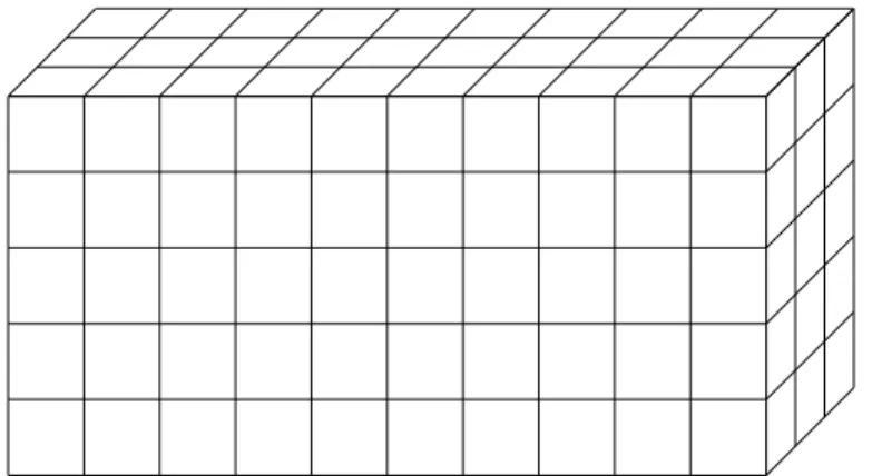
2.1 This cuboid helps to visualize a 3-tensor X ∈ _R5×10×3_{, with each small}

cube containing a scalar inR. . . 7

2.2 1-mode, 2-mode, and 3-mode unfoldings for a 3-tensorX ∈_Rn1×n2×n3_{. . .} ₁₃

2.3 matvec(X) forX ∈_Rn1×n2×n3 _{which results in a}_n 1n3×n2matrix, . . . 15

2.4 k-mode product ofX ∈ _Rn1×n2×n3 _{and matrices} _M k ∈RJk×nk. The result is Y ∈_RJ1×J2×J3_{. . . .} ₂₂

3.1 CP Decomposition for aX ∈ _Rn1×n2×n3_{. The first part shows a} tion using a sum of rank-1 tensors. The second part shows a representa-tion using factor matrices. . . 31

3.2 Tucker Decomposition forX ∈_Rn1×n2×n3_{, resulting in factor matrices with} orthogonal columns Uk ∈ Rnk×rk,k = 1,2,3 and an all-orthgonal core tensorG ∈_Rr1×r2×r3_. _{. . . .} ₃₇

3.3 PVD of a series of images M1, . . . ,Mn3. Each Mj is approximated by P·Vj·DT. . . 42

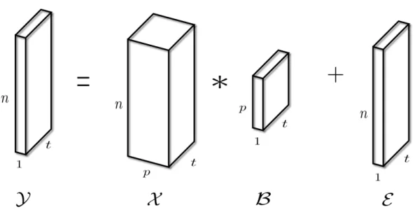
3.4 T-SVD for a X ∈ _Rn1×n2×n3_{, resulting in two orthogonal tensors -} _{U ∈} Rn1×n1×n3 andV ∈Rn2×n2×n3 - andS ∈Rn1×n2×n3 has diagonal faces alongn3. 51 5.1 Tensor Linear Model (TLM) forY ∈_Rn×1×t_,_{X ∈} Rn×p×t, andB ∈ Rp×1×t. 60 5.2 Lip Acceleration from the “Lips” Dataset . . . 79

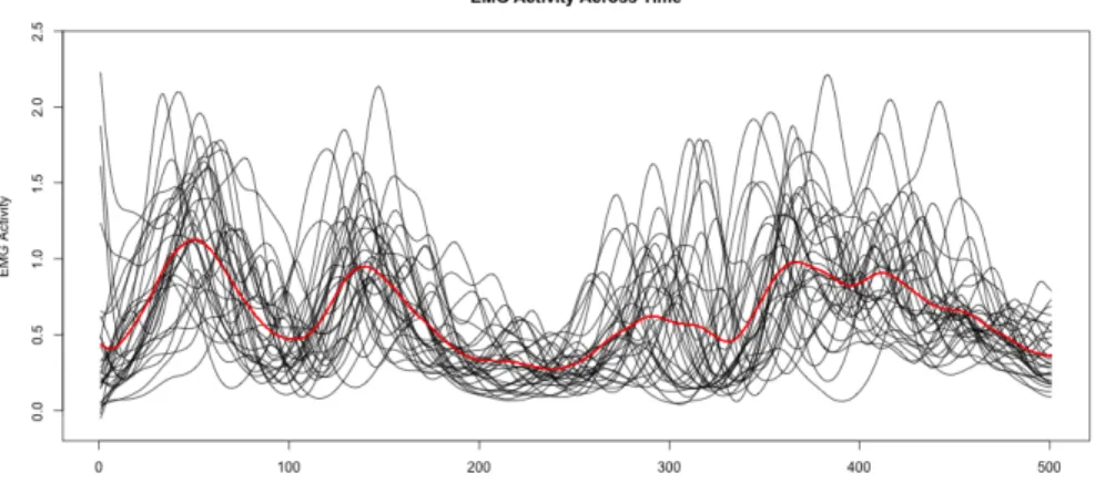
5.3 EMG Activity from the “Lips” Dataset . . . 80

5.4 Lip Position From the “Lips” Dataset . . . 80

5.5 Sample Estimated (Red) Curves Compared to the Original (Black) Curves 81 5.6 All Estimated Curves Compared to All Original Curves . . . 82

5.7 Varying Degrees ofλfor Ridge TLM . . . 83

5.8 All Out-Sample Curves Compared to All Predicted Curves . . . 84

6.1 Slots in theTensorS4 Class . . . 91

6.2 Methods inarrayoverwritten byTensor . . . 92

6.3 Methods new toTensor . . . 92

6.4 Tensor Decompositions inrTensor . . . 101

6.5 CP decomposition with 50 components and 10 components on subject 14 in the ORL Face Dataset. Picture 1 shown. Left: Original. Middle: 50 components. Right:10 components. . . 103 6.6 PVD model with various ranks on subject 8 in the ORL Face Dataset.

Picture 4 shown. Left: Original. Middle: l1 = . . . = ln3 = r1 = 46,h1 = . . . = hn3 = r2 = 56. Right: l1 = . . . = ln3 = 46,h1 = . . . = hn3 = 56,r1 =

(10)

6.7 GLRAM with various ranks on subject 21 in the ORL Face Dataset. Picture 2 shown. Left: Original. Middle: r₁ = 46,r₂ = 56. Right: r1 =23,r2= 28. . . 106

6.8 MPCA with various ranks on the entire ORL Face Dataset. Subject 35, picture 8 shown. Left:Original. Middle: r₁ =46,r₂ =56,r₃= 20. Right: r1 =46,r2= 56,r3 =10. . . 107

6.9 HOOI with various ranks on the entire ORL Face Dataset. Subject 11, picture 6 shown. Left:Original. Middle: r₁= 46,r₂ =56,r₃= 35,r₄ =8. Right: r1= 23,r2 =28,r3= 10,r4 =3. . . 108

(11)

CHAPTER 1 INTRODUCTION

There are two typical paths when one conducts data analysis. The first path is concerned withmaking reasonable inferencefrom the data, drawing conclusions about the model that generated the data, and assessing said conclusions using probability distributions and/or goodness-of-fit tests. The community that favor this path generally call themselves Statis-ticians. The second path is more concerned with using the data to build algorithmic ap-proaches that have the best possible predictive accuracy, preferably out-of-sample ac-curacy. The community that generally favor this second path call the process Machine Learning.

These two fields are not exclusive: Statisticians also want to make accurate predictions, and machine learners (sometimes) care about inferring underlying structure of the data generative process as well. However, the two camps can be readily distinguished by what is their primary concern. This is a statistics thesis, but tensor methodology is heavily used and influenced by image analysis - traditionally a subset of machine learning - where predictive accuracy in certain tasks (such as facial recognition) is the holy grail. As such, this thesis aims to contribute something to both communities.

Whether one is looking to do statistical inference or machine learning, one starts with the data. The shape, size, and source of the data often dictate the appropriate statistical methodology (or machine learning algorithm). Advances in medical imaging technol-ogy as well as telecommunication data-collection have ushered in massive datasets that

(12)

make multidimensional data more commonplace. The multidimensional structure of these datasets give impetus for new techniques that preserve the dimensionality of the data while still tying into the familiar framework of statistical inference and learning.

This thesis puts together various models used in image analysis under a tensor frame-work for statistical analysis, introduces a novel regression approach that utilize three-dimensional datasets, and develops a R package designed to facilitate the usage of tensor models amongst R users. We also address the issue of shrinkage estimation in light of our tensor regression model, and demonstrate its applications to functional data analysis.

1.1

Multilinear Data Analysis

Tensor (or multilinear) data analysis first received attention in the 1960s in psychometrics literature [53, 13, 23]. It was picked up in chemometrics beginning in the 1970s [5] and since then, tensor methods been heavily developed in that field. See Bro [10] for a recent exposition into tensor usage in chemometrics. Many papers already exist for cataloging and surveying the use of tensor techniques, with recent examples such as [28, 30, 39, 55, 20]. In particular, Kolda and Bader [30] gave a very comprehensive list of references of tensor use, noting how tensor analysis has appeared in fields such as signal processing, applied mathematics, computer vision, and data mining.

Tensor methodology has recently started to appear in statistical modeling literature as well, often under the guise of “multidimensional arrays” or “higher-order arrays”. Currie

(13)

et. al. (2006) developed the “General Linear Array Model (GLAM)” for use in multi-dimensional smoothing [15]. Hoff (2011) [24] combined the tensor framework with a bayesian estimation scheme to estimate relational data. Zhou et al. (2012) [65] developed a regression model using tensor inputs and univariate responses, applying it to neuroimag-ing data. Zhou and Li then showed in [64] (2014) how to incorporate spectral regular-ization into these tensor models. Another notable development is the Population Value Decomposition model [14], developed by Crainiceanu et al. (2011). While not directly using a tensor setup, we believe (and show) that PVD reflects a variant on the general theme of a class of tensor models.

The tensor framework seems to be the correct way of generalizing the familiar notions of vectors and matrices. While flattening of the the data (treating one or more of the levels as simply more observations or more variables) and then applying traditional matrix-based methods have been proposed and often used [58, 61], methods that do not reduce the structural integrity of the data often outperform in both model parsimony and predictive performance [55, 52, 34, 33]. In fact, many of the techniques that have been developed in lieu of a formal tensor setup are later shown to be special cases of models based on the tensor structure [52], which further strengthens the claim that tensors are the natural extension to accommodate the multilinearity of today’s Big Data.

These results, coupled with the rise in tensor usage in machine learning literature -both data mining [1, 60, 2, 45, 3] and computation [37, 19, 25] - warrant a much more unified framework for tensor methodology in the statistical community.

(14)

view and analyze tensors. We believe that this formulation of tensor multiplication based on the circulant convolution provides a new linear framework around tensors that makes it especially suitable to develop the tensor counterparts to our usual tools of projection, regression, and asymptotics. Using this novel tensor multiplication, we develop a tensor regression model that has many of the desirable properties of the Ordinary Least Squares in the case of matrix input.

1.2

Thesis Overview

The remainder of this thesis is organized as follows:

Chapter 2 will provide the relevant linear and multilinear algebra that will be used. We start by introducing the notation for the remainder of the thesis in Section 2.1, as well as the relevant matrix algebra in Section 2.2. We then provide an overview of various matrix unfolding of tensors in Section 2.3 and two major tensor multiplications in Section 2.4. We conclude the chapter with a discussion of how the two tensor multiplication differs in Section 2.5.

Chapter 3 then presents many of the most widely-used tensor decompositions and con-duct a structural comparison between them and some recent statistical models that have been introduced outside the tensor context. We cover the CP decomposition in Section 3.1, the more general Tucker decomposition in Section 3.2, Generalized Low Rank Ap-proximation (GLRAM), Multilinear Principal Component Analysis (MPCA), and 2d PCA

(15)

in Section 3.3, the Population Value Decomposition (PVD) in Section 3.4, and the Tensor Singular Value Decomposition (T-SVD) in Section 3.5.

Chapter 4 is a brief survey of multilinear tensor regression models. We cover the Tensor Regression model in Section 4.1, the Generalized Linear Array Model in Section 4.2, and end by introducing the Multilinear Normal Distribution in Section 4.3.

We motivate a novel linear model for tensors with 3 modes in Chapter 5. We first introduce the model setup in Section 5.1, then provide some algebraic results for tensors with 3 modes in Section 5.2. We then derive the least squares estimator for our model in Section 5.3 and provide an efficient FFT-based estimation algorithm in Section 5.4. We end the chapter by applying our model to a functional dataset in Section 5.5 and discussing next steps in Section 5.6.

In Chapter 6, we give a detailed look at the software we designed for tensor modeling and manipulation. In Section 6.1 we first provide an overview of available tensor software across multiple computing platforms. We then introducerTensor, our ownR[47] pack-age in Section 6.2. We discuss our choice of the S4 Class forrTensor in Section 6.3. In Section 6.4, we show how to create a tensor and convert from other objects. In Section 6.5, we show how to unfold a Tensor object as well as perform tensor multiplication. In Section 6.6, we demonstrate the various tensor decompositions available in our software, and finally in Section 6.7, we demonstrate the operations specific to tensors of 3 modes.

We conclude the thesis in Chapter 7 with a summary of contributions in Section 7.1 and suggestions for future research in Section 7.2.

(16)

CHAPTER 2 TENSOR ALGEBRA

2.1

Definitions and Notation

Tensors are also known asmultidimensional arraysorhigher-order arrays. The modes of a tensor correspond to the dimensions of a multidimensional array. Decompositions of higher-order tensors are often calledmultiway analysisormultilinear models. We now give a mathematical definition.

Defintion 1. A tensor with K modes over a field F (denoted K-tensorF) is an arranged

array of numbers, where each number is a scalar from_F. Themodes of a K-tensor_Fare the extents or dimensions of the tensor.

In this thesis we are primarily concerned withF=R, although there are a few instances whereF=C. In those instances the distinction will be clear, so we will assume thatF=R and drop the subscript for notational simplicity from now on.

Let K denote the number of modes for a tensor, and letn₁×n₂×. . .×nK denote the

modes or the extents associated with a K-tensor. Letnk specify the extent of the tensor

along thekth_{mode, and let}_i

k denote thekthindex such that 1≤ ik ≤nk, 1≤ k≤ K.

We denote a tensor with K ≥ 3 modes using the \mathcal calligraphy font, e.g.

(17)

letters, e.g.X ∈_Rn1×n2_{. We denote vectors (1-tensors) using bolded lower case letters, e.g.} x∈_Rn1 _{and scalars (0-tensors) using non-bolded lower case letters, e.g.} _x_∈

R.

Since we work mostly with 3-tensors in this thesis, it is also beneficial to define the following. Let asliceofX ∈_Rn1×n2×n3 _{be a matrix obtained by fixing one index of}_X_and leaving the remaining two free. Let atubeofXbe a vector obtained by fixing two indices and leaving one free. Denote free indices using : and subsetting operations of a tensor using brackets following the tensor.

For instance, X[:,:,1] is the first slice ofX along the third mode, andX[:,5,:] is the fifth slice ofXalong the second mode. AlsoX[:,3,4] is a vector obtained by fixingn₂ =3 andn₃ =4.

Figure 2.1: This cuboid helps to visualize a 3-tensorX ∈ _R5×10×3_{, with each small cube}

containing a scalar inR.

TheFrobenius normofX ∈_Rn1×n2×...×nK _{extends the matrix case in the usual manner:}

||X||2_F := n1 X 1= n2 X 2= . . . nK X K= x2_i 1,...,iK.

(18)

The inner product between two tensors of the same modes also extends the matrix case in the usual manner. LetX,Y ∈_Rn1×n2×...×nK_{, then}

hX,Yi:= v t n1 X i1=1 n2 X i2=1 . . . nK X iK=1 xi1,...,iKyi1,...,iK.

Addition and subtraction are defined element-wise for tensors of the same modes.

That is, givenX,Y ∈_Rn1×n2×...×nK_:

(X ± Y)i1,...,iK :=Xi1,...,iK ± Yi1,...,iK, , 1≤ik ≤ nk,1≤k≤ K.

Note that although these definitions have been provided for real-valued tensors, complex-valued tensors also have the same properties.

2.2

Relevant Matrix Algebra

In this section, we provide formal definitions for the matrix operations and structures that play crucial roles in understanding tensor operations from a matrix perspective.

Defintion 2. If A∈_Rn1×n2 _{and B}_∈

Rn3×n4, then theKronecker productof A and B is:

A⊗B=                              a11B a12B . . . a1n1B a21B a22B . . . a2n1B ... ... ... ... am11B am12B . . . am1n1B                              ∈_Rn1n3×n2n4.

(19)

Now if A,B had the same number of columns (i.e. n = n2 = n4), then the Khatri-Rao

productof A and B is defined to be the column-wise Kronecker product:

AB=

a1⊗b1. . .an⊗bn

∈_Rn1n3×n.

Finally if A,B had the exact same dimensions (i.e. m = n₁ = n₃,n = n₂ = n₄), then the

Hamadard productof A and B is defined to be the element-wise product:

A∗B=                     a₁₁b₁₁ . . . a_1nb_1n ... ... ... a_m1b_m1 . . . amnbmn                     ∈_Rm×n.

We also define another special matrix structure known as the circulant matrix that is relevant for both tensor decompositions and regression. A circulant matrix A ∈ _Rn×n is a special type of Topelitz matrix where each column of A can be obtained by shifting the previous column down one value.

Defintion 3. Acirculant matrixA∈_Rn×n_{is a square matrix fully specified by a vector of}

length n,v= v1 v2 v3. . . vn T : A= circ(v)=                                      v1 vn vn−1 . . . v2 v2 v1 vn . . . v3 v₃ v₂ v₁ . . . v₄ ... ... ... ... ... vn vn−1 vn−2 . . . v1                                     

(20)

Fourier Transform (DFT), a widely used transform. We use the definition from a classical text [9]. Defintion 4. Letv= v₁ v₂ v₃. . . vn

∈_Rn_{, then the}_{Discrete Fourier Transform}_of_v

is the sequencef ∈_Rn_{, where}

fj = n−1 X

k=0

vke−i2πjk/n.

The Fast Fourier Transform (FFT), denoted fft(v), computes the DFT quickly and

effi-ciently. The FFT ofvcan also be seen as a left multiplication by the Vandermonde matrix

Fn =                              ω0·0 n ω0 ·1 n . . . ω 0·(n−1) n ω1·0 n ω1 ·1 n . . . ω 1·(n−1) n ... ... ... ... ω(n−1)·0 n ω (n−1)·1 n . . . ω (n−1)·(n−1) n                              ,

whereωn = e−i2π/n. The inverse FFT, denoted iff(f), can be seen as a left multiplication

by the complex conjugate of Fn, which we denote F∗n. Hence we havefj = (Fn ·v)j and

vj =(F∗n·f)j.

A circulant matrixAspecified byv∈_Rn_{can be diagonalized by}_F

n as follows: F∗_n·A·Fn = 1 n                              f1 f2 ... fn                             

Now with a series of matricesA₁,A₂, . . . ,An, we can similarly construct a block

(21)

Defintion 5. A block circulant matrix A ∈ _Rn1n3×n2n3 _{is fully specified by a series of n} 3 matrices A₁,A₂, . . . ,An3, each Aj ∈R n1×n2_: A=                                      A₁ An3 An3−1 . . . A2 A₂ A₁ An3 . . . A3 A3 A2 A1 . . . A4 ... ... ... ... ... An3 An3−1 An3−2 . . . A1                                      .

Similar to the circulant matrix, the block circulant matrix can be block diagonalized byFn[27]: (F∗_n 3 ⊗In1)·A·(Fn3 ⊗In2)= 1 n                              D₁ D₂ ... Dn3                              ,

where eachDj ∈ Cn1×n2 has a special structure that is discussed in more depth in Section

2.4.2.

2.3

Tensor Unfolding

ForK ≥ 3, it is often useful to be able to represent aK-tensor as a matrix or as a vector, especially as a first step in defining a tensor multiplication. This representation is often called unfolding or flattening. As we will see in Section 2.4, tensor unfolding allows us to

(22)

on the tensor unfolding operations that have been used predominantly in tensor analysis, and then describe a general way of thinking about tensor unfolding that connects these seemingly disparate operations.

First consider the vector representation of aK-tensor, which is simply a stacking of the K-tensor element-wise into a n₁n₂. . .nK vector. A useful convention is to allow the last

index to vary the fastest and the first index to vary the slowest. This prompts the following natural definition.

Defintion 6. For aX ∈ _Rn1×n2×...×nK_{, the}_{vectorization}_of_X_{, denoted}_vec(_X_{), is the} opera-tion that creates a vector of length n₁n₂. . .nK from the elements ofX, ordered according

to the convention that allows iato vary faster than ib for K≥ a>b≥1.

For instance, for a 3-tensorX ∈_Rn1×n2×n3_,

vec(X)=                                                        x₁₁₁ x₁₁₂ ... x121 x122 ... xn1n2n3                                                        ∈_Rn1n2n3.

Now consider how a general K-tensor can be represented in matrix form. One defi-nition that has prevailed in earlier tensor literature is thek-mode matricization/unfolding [28].

(23)

Defintion 7. ForX ∈ _Rn1×n2×...×nK_{, denote}_X

(k) ∈ Rnk×

Q

j,knj _{to be the k}_{-mode unfolding}_.

X_(k) is a mapping from the (i1,i2, . . . ,iK)th element to the(ik, j)th element of the resulting

matrix, where j=1+ K X p_,k (ip−1)Jp, with Jp= p−1 Y q_,k nq,

ordered according to the convention that allows iato vary faster than ibfor K ≥a> b≥ 1.

The convention in the permutation of the indices{n₁, . . . ,nk−1,nk+1, . . . ,nK}is

consis-tent to the convention from the vec(·) operation. For a 3-tensor, there are three k-mode unfoldings, denotedX₍₁₎,X₍₂₎, andX₍₃₎, all of which are demonstrated in Figure 2.2.

(24)

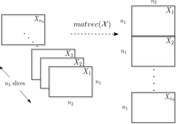
Kilmer et. al. proposed another tensor unfolding known as the matvec(·) operation [27]. Similar to how vec(·) of a matrix stacks its columns to form a vector, matvec(·) of a 3-tensor stacks the slices (2-tensors) along the third mode and stacks them to form a matrix.

Defintion 8. ForX ∈ _Rn1×n2×n3_{, let X}

j := X[:,:, j], j = 1, . . . ,n3, then thematrix

vector-izationofX, denotedmatvec(X), is

matvec(X)=                     X₁ ... Xn3                     ∈_Rn1n3×n2.

(25)

Figure 2.3: matvec(X) forX ∈_Rn1×n2×n3 _{which results in a}_n

1n3×n2matrix,

While matvec(·) is also defined for generalK-tensors[42], it does not result in a matrix, so we do not elaborate on that in this paper.

We now define a more general way of considering tensor unfolding which provides additional insight into the differences between the matvec(·) andk-mode unfolding. We first define aK-tensor generalization of a tube.

Defintion 9. For anyX ∈ _Rn1×n2×...×nK_{, let the k}_{-mode vectors} _{be the vectors indexed by}

(26)

mode. Denote these as

X[i1, . . . ,ik−1,:,ik+1, . . . ,iK]∈Rnk,1≤ ij ≤ nk,1≤ k≤ K.

We can now define the row/column space unfolding of a tensor.

Defintion 10. The row space unfolding of X in the mode k, denoted unfoldRS(·,k), is

the stacking of all k-mode vectors ofX as columns in the resulting matrix. Similarly, the

column space unfolding ofXin the modek, denotedunfoldCS(·,k), is the stacking of all

k-mode vectors as rows in the resulting matrix. For anyX ∈_Rn1×n2×...×nK_,

unfoldRS(X,k)∈Rnk×( Q j,knj)_{, and} unfoldCS(X,k)∈R( Q j,knj)×nk.

Furthermore,(unfoldRS(X,k))T =unfoldCS(X,k).

As an example, considerX ∈_R3×4×5_{; the row space unfoldings are:}

unfoldRS(X,1)=

X[:,1,1] X[:,1,2] . . . X[:,1,5] X[:,2,1] . . . X[:,4,5]

| {z } 20 columns vectors of length 3

unfoldRS(X,2)=

X[1,:,1] X[1,:,2] . . . X[1,:,5] X[2,:,1] . . . X[3,:,5]

unfoldRS(X,3)=

X[1,1,:] X[1,2,:] . . . X[1,4,:] X[2,1,:] . . . X[3,4,:]

(27)

and the columns space unfoldings are: unfoldCS(X,1)=                                                        X[:,1,1]T X[:,1,2]T . . . X[:,1,5]T X[:,2,1]T . . . X[:,4,5]T                                                        | {z } 20 row vectors of length 3

unfoldCS(X,2)=                                                        X[1,:,1]T X[1,:,2]T . . . X[1,:,5]T X[2,:,1]T . . . X[3,:,5]T                                                        | {z } 15 row vectors of length 4

(28)

unfoldCS(X,3)=                                                        X[1,1,:]T X[1,2,:]T . . . X[1,4,:]T X[2,1,:]T . . . X[3,4,:]T                                                        | {z } 12 row vectors of length 5

.

These two definitions allow us to better juxtapose thek-mode unfolding of a 3-tensorX

and the matvec(·), since the former is exactly the same as the row space unfolding in thekth

mode while the latter is exactly the same as column space unfolding in the second mode. Hence, the main difference between these two unfolding operations can be attributed to whether we stack thek-mode vectors as rows or columns.

The folding operations, which invert these unfold operations, are defined through the unfolding themselves. It is important to note that the foldings operate on any arbitrary matrix, so it becomes necessary to specify the exact modes of the resulting tensor.

Defintion 11. Let the folding operation of matrices into tensors as the inverse operations

to the corresponding tensor unfolding, and let mn= QK_k₌₁nk. Therow space folding of a

matrix in the modek for X ∈_Rm×n _is

foldRS(X,k,n1×n2×. . .×nK)=X ∈Rn1×n2×...×nK,

where X =unfoldRS(X,k). Similarly, definecolumnn space foldingof X ∈Rm×nto be

(29)

where X =unfoldCS(X,k).

Another way to explicitly represent these tensor unfoldings is with the use of basis vectors and Kronecker notation. First letej ∈R1×n be the jth column unit basis vector of

lengthnandeT_j ∈_Rn×1be the row unit basis vector of lengthn. For notational convenience, we dropped the length of the basis vectors where it is unambiguous to do so.

Now any matrixX ∈_Rn1×n2 _{can be written as a sum of its scalar elements:} X = n1 X i=1 n2 X j=1 (ei⊗eTj)Xi j.

Furthermore, we can now write down the vec(X)∈_Rn1n2 _as vec(X)= n1 X i=1 n2 X j=1 (ei⊗ej)Xi j.

We see that the row and column basis vectors allow us to explicitly “pick off” the individual elements of the matrix and re-arrange them.

Now for X ∈ _Rn1×n2×n3_{, we can use these to explicitly write down the three} _k-mode unfoldings of the 3-tensor:

X₍₁₎= n1 X i=1 n2 X j=1 n3 X k=1 (ei⊗eTj ⊗e T k)Xi jk X₍₂₎= n1 X i=1 n2 X j=1 n3 X k=1 (eT_i ⊗ej⊗eTk)Xi jk X₍₃₎= n1 X i=1 n2 X j=1 n3 X k=1 (eTi ⊗e T j ⊗ek)Xi jk,

(30)

as well as the matvec(·) and vec(·): matvec(X)= n1 X i=1 n2 X j=1 n3 X k=1 (ei ⊗eTj ⊗ek)Xi jk, vec(X)= n1 X i=1 n2 X j=1 n3 X k=1 (ei ⊗ej⊗ek)Xi jk.

This extends to generalK-tensors and the row/column space definition as well: unfoldRS(X,k)= n1 X i1=1 n2 X i2=1 . . . nK X iK=1 (eTi1 ⊗e T i2 ⊗. . .⊗e T ik−1 ⊗eik ⊗e T ik+1 ⊗. . .e T iK)Xi1,...,iK unfoldCS(X,k)= n1 X i1=1 n2 X i2=1 . . . nK X iK=1 (ei1 ⊗ei2 ⊗. . .⊗eik−1 ⊗e T ik ⊗eik+1 ⊗. . .eiK)Xi1,...,iK vec(X)= N1 X i1=1 N2 X i2=1 . . . NK X iK=1 (ei1 ⊗ei2 ⊗. . .⊗eik)Xi1,...,iK

2.4

Tensor Multiplication

In this section, we discuss two prevailing definitions of tensor products - thek-mode mul-tiplication and thet-product - and illustrate the crucial differences.

2.4.1

k

-mode Product

We start with the definition.

Defintion 12. The k-mode product specifies multiplication between a K-tensor X ∈

(31)

a K-tensor in_Rn1×...×nk−1×J×nk+1×...×nK_{. This is defined element-wise to be:} (X ×k M)i1,...,ik−1,j,ik+1,...,iK = nk X ik=1 Xi1,...,iKMj,ik.

As the name suggests, this product definition is closely related to thek-mode unfolding. In fact:

Y =X ×k M ⇔ Y(k)= M· X(k),

where·denotes the usual matrix multiplication.

In other words, we can think about thek-mode product as a left matrix multiplication onto the k-mode vectors: each k-mode vector of the resulting tensor Y is a result of a matrix-vector multiplication betweenMand the correspondingk-mode vector ofX. Note that if M is a vector (i.e. J = 1), then eachk-mode vector ofY is the result of an inner product between two vectors, andYwill havenk =1 and is essentially a (K−1)-tensor.

(32)

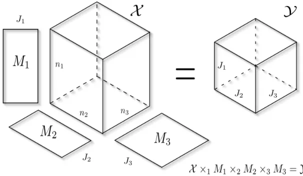
Figure 2.4: k-mode product of X ∈ _Rn1×n2×n3 _{and matrices} _M

k ∈ RJk×nk. The result is Y ∈_RJ1×J2×J3_.

Also note that if X ∈ _Rn1×n2 _{were a matrix, then the} _{k-mode product between} _X _and M₁∈_RJ1×n1,_M

2 ∈RJ2×n2 is equivalent to the following matrix products:

X×₁ M₁ = M₁T·X ∈_RJ1×n2 X×₂ M₂ =X· M₂ ∈_Rn1×J2

Thek-mode product serves as the basis for many tensor decompositions and regression models, including the Tucker decomposition and the CP decomposition. It also bears mentioning that the Kronecker product permits a matrix view of the product between a

(33)

generalK-tensor and a list of matrices [28]:

Y =X ×₁ M₁×₂M₂. . .×K MK

⇔Y_(k)= Mk· X(k)·(MK ⊗. . .⊗ Mk+1⊗ Mk−1. . .⊗M1)T

For more properties of thek-mode product, see [28].

2.4.2

t

-Product

While thek-mode product defines multiplication between a tensor and a matrix, it does not provide a natural way to multiply two 3-tensors. To this end, thet-product has recently been proposed by [27]. We believe this latter tensor product shows great promise in its applicability to statistical modeling and regression. Prior to exploration of thet-product, however, we need to recall the block circulant matrix structure from Section 2.2.

We can couple the block circulant structure with the matvec(·) operation to create a block circulant matrix using the slices of a 3-tensor along mode 3. LetX ∈_Rn1×n2×n3_{, then:}

circ(matvec(X))=                                      X1 Xn3 Xn3−1 . . . X2 X2 X1 Xn3 . . . X3 X3 X2 X1 . . . X4 ... ... ... ... ... Xn3 Xn3−1 Xn3−2 . . . X1                                      ,

(34)

means that forX ∈_Rn1×n2×n3_,

(F∗n3 ⊗In1)·circ(matvec(X))·(Fn3⊗In2)= diag(D1, . . . ,Dn3),

whereFnis thenthorder discrete Fourier transform matrix andDj ∈Cn1×n2. It is important

to note thatDj = D[:,:, j], whereD ∈ Rn1×n2×n3 is created vian1×n2FFT’s: D[i1,i2,:]=

Fn3(X[i1,i2,:]). Thet-product is defined via the block circulant structure and the matvec(·) operator and allows for a direct multiplication of two 3-tensors.

Defintion 13. For A ∈ _Rn1×n2×n3 _and _{B ∈}

Rn2×L×n3, the t-productis A ∗ B ∈ Rn1×L×n3, where thematvec(A ∗ B)is a result of matrix multiplication:

matvec(A ∗ B)= circ(matvec(A))·matvec(B)

=                                      A₁ An3 An3−1 . . . A2 A₂ A₁ An3 . . . A3 A₃ A₂ A₁ . . . A₄ ... ... ... ... ... An3 An3−1 An3−2 . . . A1                                      ·                                      B₁ B₂ B₃ ... Bn3                                      ∈_Rn1n3×L. _(2.1)

Here Aj = A[:,:, j],Bj =B[:,:, j]are the jthslices ofAandBalong mode 3 respectively.

To get the tensorA ∗ B, we simply have to foldmatvec(A ∗ B)using the inverse folding formatvec(·). Since we noted that thematvec(·)operation is equivalent tounfoldCS(·,2),

then we haveA ∗ B=foldCS(matvec(A ∗ B),2,n1×L×n3).

From the definition of thet-product, we can see that each mode-3 slice of the resulting tensor A ∗ B is given by a sum of products of the mode-3 slices of A and B. In fact, thet-productA ∗ B defines a linear map that takesB ∈ _Rn2×L×n3 _to

(35)

allows the extension of familiar linear algebra concepts such as the transpose, orthgonality, nullspace, and range. For detailed accounts of these properties, refer to [27]. Whenn₃= 1, we get back the usual matrix multiplication.

For general K-tensors, where K ≥ 4, the t-product is extended in [42] to be defined recursively with the base case being the 3-tensor t-product. For instance, for 4-tensors

A ∈_Rn1×n2×n3×n4,_{B ∈} Rn3×L×n3×n4, we have A ∗ B:=foldCS(                                      A1 An3 An3−1 . . . A2 A₂ A₁ An3 . . . A3 A₃ A₂ A₁ . . . A₄ ... ... ... ... ... An3 An3−1 An3−2 . . . A1                                      ∗                                      B1 B₂ B₃ ... Bn3                                      )∈_Rn1×L×n3×n4,

where eachAj ∈ Rn1×n2×n3 andBj ∈ Rn2×L×n3 are the jth sub-tensors of A and Balong

the 4th mode respectively, andAi ∗ Bj is defined as in Equation 2.1, ∀i, j ∈ {1, . . . ,n4}.

Once again, thet-product has the characteristic that every sub-tensor ofBis hit by every sub-tensor ofA.

Our earlier note regarding the DFT block-diagonalization plays a crucial role in in-creasing the computation efficiency of thet-product, as it reduces both time and storage costs. Using the DFT, one does not need to construct the full block circulant matrix from

(36)

Algorithm 1t-Product for 3-Tensors input :A ∈_Rn1×n2×n3_,_{B ∈} Rn2×L×n3 fori1 =1, . . . ,n1 do fori₂ =1, . . . ,n₂do ˜ A[i1,i2,:]=fft(A[i1,i2,:]) end fori₂ =1, . . . ,Ldo ˜ B[i1,i2,:]=fft(B[i1,i2,:]) end end for j=1, . . . ,n3 do ˜ C[:,:, j]=A˜[:,:, j]·B˜[:,:, j] end fori1 =1, . . . ,n1 do fori₂ =1, . . . ,Ldo C[i1,i2,:]=ifft(C[i1,i2,:]) end end output :C= A ∗ B ∈_Rn1×L×n3

The DFT block-diagonalization technique also makes tensor decompositions involv-ing thet-product much more efficient. Note however, that the the DFT transform is not necessary in the definition oft-product; it is only a computation aid to increase both speed and storage efficiency of the operation.

2.5

Linear versus Multilinear

A natural question to ask about the two different tensor products defined above is how do they differ? Aside from the obvious structural differences between the two, the crucial

(37)

distinction is that while the t-product defines a linear map for a K-tensor, the k-mode product defines amultilinear map[27] for a list of matrices.

To be explicit, consider the case whereK = 3. Thet-product betweenA ∈ _Rn1×n2×n3 andB ∈_Rn2×L×n3 _{defines a linear map}

Rn2×L×n3 7→ Rn1×L×n3 via the operationA ∗ B. When n₃ = 1, then the t-product reduces to the usual matrix product between A ∈ _Rn1×n2 _and B∈_Rn2×L_{, which is a linear map for}

Rn2×L 7→Rn1×Lvia the operationA·B.

On the other hand, a multilinear map takes multiple arguments and is linear in each of the argumentsseparately. Thek-mode product betweenA ∈ _Rn1×n2×n3 _{and a list of matrices} Mk ∈RJk×nk,1≤ k ≤3, defines a map that is linear in eachRJk×nk 7→ RJk×

Q

j,knj _separately via a change of basis onA ×k Mk.

A consequence of this distinction is that the k-mode product treats all the modes of the original tensor in exactly the same way, whilet-product does not; the ordering of the modes on the 3-tensor matters for thet-product. This should not be surprising as ordering also matters when it comes to matrix multiplication. As we will see in the next section, both thet-product and thek-mode product facilitate decomposition models for tensors, by allowing “lower rank approximations” of tensors similar to the matrix versions. However, only thet-product will allow us to construct a linear model using tensors, while thek-mode product is meant to construct multilinear models.

(38)

CHAPTER 3

TENSOR DECOMPOSITIONS

In this chapter, we describe and contrast notable tensor decompositions. These decom-position models represent the bulk of the tensor methodology used in facial recognition, data-mining, and statistical analysis of image populations.

Tensor decompositions have been predominantly multilinear, and we start with these more traditional decompositions. In Section 3.1 we discuss the CP decomposition, which introduced the notion of a tensor rank. In Section 3.2 we discuss the more general Tucker decomposition, which encompasses CP as a special case. In Section 3.3 and Section 3.4, we discuss two matrix-based models that actually have intimate connections with the Tucker model. Finally, in Section 3.5, we discuss Tensor Singular Value Decomposition (T-SVD) [27], a novel method based on thet-product, as well as related Tensor approxi-mation schemes. Whereas the family of Tucker models decomposes a higher-order tensor into a higher-order core and factor matrices for each mode, the T-SVD decomposes into multiple higher-order tensors.

3.1

CP

The CP decomposition stemmed independently from psychometrics [13] and chemomet-rics [10], where the same method was separately named Canonical Decomposition (CAN-DECOMP) and Parallel Factors (PARAFAC). We first describe the related concept of

(39)

ten-sor rank.

AK-tensorX ∈ _Rn1×n2×...×nK _{is called rank-1 if it can be expressed as an outer product} ofKvectors. It is called rank-rif it can be expressed as a sum ofrrank-1K-tensors:

X=

r X

`=1

v1`◦v2`. . .◦vK`, wherevk` ∈Rnk,1≤ ` ≤r,1≤k≤ K.

For matrices, the well-known Eckhart Young Theorem provides the existence and form of an optimal lower-rank approximation. However, this type of result has been shown not to generalize toK-tensors forK ≥3 [29].

Fortunately, the CP decomposition provides an approximation of X using a rank-r tensor ˆX, where r is given a priori. The goal is then to construct a rank-r tensor that minimizes the Frobenius norm of the difference betweenXand ˆX:

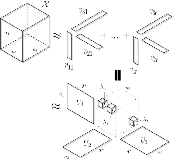
min alluk` ||X −X||ˆ F, where ˆ X= r X `=1 v1`◦v2`. . .◦vK` (3.1) = r X `=1 λ`·u1`◦u2`. . .◦uK`,uk` = vk` ||vk`|| (3.2) = Λ×₁U₁×₂U₂×₃. . .×KUK, where (3.3) Uk = uk1 uk2 . . . ukr ∈_Rnk×r,₁_≤ _k_≤ K, and Λ∈_Rr×r×r

(40)

The equivalence of lines (3.1) and (3.2) are due to the fact that eachuk` vector is vk`

normalized by its norm with the norm information stored in the λr’s. Furthermore, we

can store theuir vectors as a factor matrix Uk for each k = 1, . . . ,K [32], leading to the

form in line (3.3). Note that here theUk matrices are not orthogonal. This relationship is

(41)

Figure 3.1: CP Decomposition for a X ∈ _Rn1×n2×n3_{. The first part shows a} representa-tion using a sum of rank-1 tensors. The second part shows a representarepresenta-tion using factor matrices.

A large body of literature has been devoted to obtaining ˆXwith various possible solu-tions ranging from iterative to closed-formed [33, 32, 11, 51]. Some methods also exist to

(42)

We consider the basic iterative procedure known as alternating least squares (ALS), as described in [28]. ALS for a 3-tensor proceeds with choosing some starting values for matricesU₁,U₂,U₃. Then at each iteration, we hold two of these matrices fixed and minimize||X−X||ˆ Fwith respect to the third matrix, then repeat across the other two modes.

For instance, if we holdU₂,U₃constant thenU₁has a closed form best approximation: Set ˆX₍₁₎ =U1·Λ(1)·(U3⊗U2)T Setting ∂(||X − ˆ X||F) ∂U1 =0⇒ ˆ U₁ =Xˆ₍₁₎·[(U3⊗U2)T] † =_Xˆ₍₁₎_·_(U₃_U₂₎_·_(UT 2U2∗UT3U3)†,

where† denotes the Moore-Penrose Pseudoinverse, This process is then repeated for each of the two other modes to find ˆU2 and ˆU3. The algorithm exploits connections

be-tween the Kronecker and both the Khatri-Rao () and Hamadard (∗) products of matrices [28, 55]. A usual convergence criterion is when there is a small enough difference be-tween successive||X −X||ˆ , but there is no guarantee that CP using ALS will convergence to a global minimum. This procedure is provided inrTensor[36] forX ∈_Rn1×n2×...×nK_.

(43)

Algorithm 2CP using Alternating Least Squares (CP-ALS) input :X ∈_Rn1×n2×...×nK_{, and desired rank}_r.

initialize:U₁, . . . ,UK random matrices

whileNot Convergeddo

fork =1, . . . ,Kdo H ←UT₁U1∗U₂TU2∗. . .∗UkT−1Uk−1∗U T k+1Uk+1. . .∗U T KUK Uk ← X(k)·(UK UK−1. . .Uk+1Uk−1. . .U1)·H† [λ1, . . . , λr]←norms of columns ofUk end end

output : scalarsλ1, . . . , λr, factor matricesU1, . . . ,UK, eachUk ∈Rnk×r

3.2

Tucker

The Tucker decomposition [53, 32] is still based on the idea of obtaining the best approx-imation of X, but relaxing the constraint that ˆX must be expressed as a sum ofr rank-1 tensors. Instead, the Tucker decomposition constructs ˆXto approximateX ∈ _Rn1×n2×...×nK using a reduced core tensor G ∈ _Rr1×...×rK _and _K _{factor matrices, each of rank} _r

k ≤ nk,

k=1, . . . ,K:

ˆ

X= G ×1U1×2U2×3. . .×KUK.

If this looks similar to the CP, it is because the CP decomposition can be seen as the Tucker decomposition with all the ranks equal, (i.e. r = r₁ = . . . = rK) [28]. The

gen-eral Tucker decomposition does not give a unique solution, however, so certain constraints must be placed on the factor matrices to ensure uniqueness. In this paper, we focus on Higher Order Orthogonal Iteration (HOOI) [33], which constrains the factor matrices to

(44)

be orthogonal, thus resulting in a unique solution.

Before we demonstrate HOOI, we first discuss the very much related higher-order singular value decomposition (HOSVD) provided by the seminal paper by Lathauwer et. al. [33]. HOSVD decomposes aK-tensorX ∈_Rn1×n2×...×nK _{as follows:}

X= G ×1U1×2U2×3. . .×KUK,

where each square matrixUk ∈ Rnk×nk is orthogonal and the core tensorG ∈ Rn1×n2×...×nK

has the special property that for anyk,1≤k≤ K, it is • all-orthgonal:hGik=α,Gik=βi=0 for anyα,β, and

• ordered:||Gik=1||F ≥ ||Gik=2||F ≥ . . .||Gik=nk||F.

For 3-tensors, all-orthogonality of Gmeans that for any of the three modes, any two matrix slices with different indices along that mode has an inner-product of 0. While one might expect the core tensorGto have some sort of diagonal structure, that is not the case here.

The corresponding algorithm to compute the HOSVD illustrates its crucial connection between thek-mode unfolding: for eachk-mode unfolding, perform a matrix SVD forX_(k)

so thatX_(k) =UkΣkV_kT. Now we can simply defineG:=X ×1U1T×2U2T. . .×KUTK, then G_(k) =U_nT· X_(k)·(UKT ⊗. . .⊗U T k+1⊗U T k−1⊗. . .⊗U T 1) T ⇒ X_(k) =Uk· G(k)·(UK ⊗. . .⊗Uk+1⊗Uk−1⊗. . .⊗U1)T ⇒ X=G ×₁U₁×₂U₂×₃. . .×KUK,

(45)

giving us the HOSVD. The following algorithm is implemented inrTensor[36].

Algorithm 3Higher-Order Singular Value Decomposition (HOSVD)

input :X ∈_Rn1×n2×...×nK_. fork= 1, . . . ,K do

Uk ←left orthogonal matrix of the SVD ofX(k)

end

G ← X ×1UT1 ×2U2T ×3. . .×KUTK

output : core tensorG ∈_Rn1×n2×...×nK_{, orthgonal factor matrices}_U

1, . . . ,UK, each

Uk ∈Rnk×nk

The key concept here that allows us to obtain a Tucker decomposition from HOSVD is that if we truncate eachUk to its firstrk columns for each 1 ≤ k ≤ K, then we would

end up with an approximation ofX. Successive iterations of this alternating truncation and SVD for all the modes will give us a locally optimized approximation ˆX. This is known as the higher-order orthogonal iteration (HOOI) [33] and provides an iterative scheme to find the Tucker decomposition with orthogonality constraints.

(46)

Algorithm 4Orthogonal Tucker Alternating Least Squares (HOOI) input :X ∈_Rn1×n2×...×nK_{, and desired ranks}_r

1, . . . ,rK.

initialize:U₁, . . . ,UK via HOSVD

fork =1, . . . ,Kdo Y ← X ×₁U₁T ×₂. . .×k−1UkT−1×k+1U T k+1. . .×K U T K

Uk ← rkleading singular vectors ofY(k)

end end G ← X ×₁UT 1 ×2. . .×K U T K

output : core tensor G ∈ _Rr1×...×rK_{, factor matrices with orthogonal columns}

U1, . . . ,UK, eachUk ∈Rnk×rk

Note that in many modified versions of HOOI, the truncated HOSVD only serves as an initial value. Successive iterations do not require a full SVD at each mode for the matricized tensor, but only some scheme to minimize

||X − G ×₁U₁×₂. . .×k−1Uk−1×k+1Uk+1. . .×KUK||F,

(47)

Figure 3.2: Tucker Decomposition for X ∈ _Rn1×n2×n3_{, resulting in factor matrices with} orthogonal columnsUk ∈Rnk×rk,k=1,2,3 and an all-orthgonal core tensorG ∈Rr1×r2×r3.

By allowing the specification of the ranksr1, . . . ,rK, Tucker offers more flexibility than

CP in the amount of truncation along each mode ofX. Furthermore, with HOOI, we are also given orthogonal factor matrices. These properties makes HOOI a much more attrac-tive statistical model than CP, and have lead to a number of statistical tensor regression methods, as we will see in Chapter 4.

It is important to note that in the absence of truncation, the Tucker decomposition (with orthogonality constraints) can be viewed as just the HOSVD and therefore does not require

(48)

compressed and will still be of sizen1×n2 ×. . .×nK. Since tensor decompositions are

often used to compress large tensors, this does not seem very practical. It does, however, give us a way to compare the structural changes across many different methods, as we will see in the following sections.

3.3

GLRAM, MPCA, & 2dPCA

In this section, we discuss several statistical models that are unified under the Tucker framework. While some of these models explicitly use tensor notation and methodology, others use a series of matrices as inputs.

The Generalized Low Rank Approximate of Matrices (GLRAM) [59] belongs in the latter category. For a series of matrices of the same size, M1, . . . ,Mn3 ∈ R

n1×n2_{, GLRAM} constructs orthogonal matrices L ∈ _Rn1×r1,_R _∈

Rn2×r2 and a series of core matricesGj ∈

Rr1×r2 to minimize the quantity

n3

X

j=1

||Mj− L·Gj ·RT||2F. The parametersr1 and r2 would

also need to be given a priori.

The series of images GLRAM takes as input can be restructured into a 3-tensor

X ∈ _Rn1×n2×n3_{, where}_X[:,:, _j] = _M

j. This has been done in [52], where it is shown that

when structured in this way, GLRAM becomes a special case of the Tucker decomposition with orthogonality constraints. Essentially, GLRAM performs HOOI in 2 of the 3 modes, while leaving the third mode uncompressed. To make the comparison between the matrix and tensor settings more explicit, We present the same GLRAM algorithm using both the

(49)

matrix notation and the tensor notation below:

Algorithm 5Generalized Low Rank Approximation of Matrices using matrix notation

input : Matrices M1, . . . ,Mn3, ranksr1,r2.

initialize:Lrandom matrix

FormCR = n3

X

j=1

MT_j ·L·LT ·Mj

R← r2eigenvectors corresponding to ther2largest eigenvalues ofCR

FormCL= n3

X

j=1

Mj·R·RT ·MTj

L←r1eigenvectors corresponding to ther1 largest eigenvalues ofCL

end

for j=1, . . . ,n₃ do Vj ← LT ·Mj·R

end

output :L,R,V₁, . . . ,Vn3

Algorithm 6GLRAM using tensor notation

input :X ∈_Rn1×n2×n3_{, ranks}_r

1,r2.

FormCR = X(1)· XT₍₁₎

R← r₂eigenvectors corresponding to ther₂largest eigenvalues ofCR X ← X ×₂RT

FormCL= X(2)· XT₍₂₎

L←r₁eigenvectors corresponding to ther₁ largest eigenvalues ofCL X ← X ×₁ LT end for j=1, . . . ,n₃ do Vj ← LT · X[:,:, j]·R end output :L,R,V₁, . . . ,Vn3

(50)

One can see that during GLRAM, we are essentially performing HOOI over only the first two modes, since SVD of X_(i) gives the same left eigenvectors as the eigenvalue decomposition ofX_(i)· XT

(i),i= 1,2.

When applied to a series ofK-tensors forK ≥ 3, this technique, is called Multilinear Principal Component Analysis (MPCA) [38]. MPCA is also a special case of the general Tucker decomposition forK-tensors, compressing onK−1 modes and leaving one mode uncompressed. Hence GLRAM is a special case of MPCA for 3-tensors. Notationally, MPCA is equivalent to HOOI withUK = Ink, which means that GLRAM is equivalent to HOOI withU₃= In3.

Yet another related technique is called 2-dimensional Principal Component Analysis (2dPCA) [58, 61], and that is also shown to be a special case of GLRAM [52], where two of the three modes are uncompressed (i.e. U2 = In2,U3 = In3). All the decompositions mentioned above (HOOI, GLRAM, 2dPCA, and MPCA) are available inrTensor[36].

3.4

PVD

Recently proposed by [14], the Population Value Decomposition (PVD) provides a frame-work to construct population-level factor matrices for a series of images. We show in this section that PVD actually is a variant of GLRAM. This point was first made by Lock et al. in the rejoinder of the original PVD paper [14], and Crainiceanu et al. replied that PVD differs from Tucker (or specifically, GLRAM) in many ways. Most notably, the matrices

(51)

PandDdo not have to be orthogonal and that the default PVD has a closed form solution. We first present PVD and the default algorithm suggested by the authors to construct the population matrices Pand D, then examine the differences between PVD and GLRAM. Finally, we discuss how PVD might be cast in the tensor framework.

Like GLRAM and 2dPCA, PVD is a model designed for a series of matrices instead of a 3-tensor setup. Given a sample of imagesM1, . . . ,Mn3 ∈R

n1×n2_{, and 2n}

3+2 parameters,

PVD constructs population level matrices P ∈ _Rn1×r1 _and _D _∈

Rn2×r2 such that Xj =

P·Vj·D+Ej, where theVj ∈Rr1×r2, j= 1, . . . ,n3, are called the core matrices. In addition

to the 2 parameters ri ≤ ni, i = 1,2, we also would need to choose 2n3 compression

parameters,l₁, . . . ,ln3,h1, . . . ,hn3, that will determine how much left and right truncation will occur for each of then₃matrices.

The PVD procedure starts with a separate SVD of each image,Mj =UjΣjWTj,

truncat-ing (possibly differently for each image) the left and right eigenvectors to form ˜Ujand ˜Wj.

Then the one would stack the ˜Uj’s column wise to form a big matrix U and do the same

for ˜Wj’s to formW. The final step is to conduct an eigenvalue decomposition ofU·UTand

W·WT _{to form the population level matrices}_P_and_{D. In the end, each}_M

jhas a projection ˆ Mj = P· {(PT ·U˜j)·Σ (lj,hj) n ·( ˜Wj ·DT)} | {z } Vj ·D, whereΣ(lj,hj)

(52)

Figure 3.3: PVD of a series of imagesM1, . . . ,Mn3. EachMjis approximated byP·Vj·D

T

.

Unlike the usual algorithm needed to solve GLRAM, the algorithm to solve the default PVD is not iterative, although the computational cost of the model does scale up with the number of images, since each image requires a separate SVD. Furthermore, with a largen3,

theUUT andWWT matrices may be intractable for a full eigenvalue decomposition. We present the matrix version of the default PVD algorithm below, which is fully implemented inrTensor[36].

(53)

Algorithm 7Default Population Value Decomposition (PVD)

input : Matrices M₁, . . . ,Mn3, matrix-wise ranks l1, . . . ,ln3,h1, . . . ,hn3, final ranksr1,r2. for j=1, . . . ,n3 do Perform SVD to obtain Mj = Uj·Σj·WT_j ˜ Uj ←leftljcolumns ofUj ˜ Wj ←lefthj columns ofWj end

Stack the ˜Uj column-wise to constructU = h

˜

U1 . . . U˜n3

i

and similarly stack the ˜Wj to formW = h

˜

W₁ . . . W˜n3

i

.

P←eigenvectors corresponding to ther₁leading eigenvalues ofU·UT D←eigenvectors corresponding to ther2leading eigenvalues ofW·WT

for j=1, . . . ,n₃ do Vj ← PT ·U˜j·Σ (lj,rj) j ·W˜ T j D T end output :P,D,V1, . . . ,Vn3

Since both PVD and GLRAM are designed to work on a series of imagesMj, a natural

question is how do they compare with each other. Lock et al. gave an empirical comparison of both methods on the Orville Face dataset [12]. We found that in addition to these empirical similarities, if we were to compare both these methods under the case of no truncation, (i.e. no compression on any modes), then a striking similarity emerged.

First consider a GLRAM model for X with ranks r₁ = n₁,r₂ = n₂. This amounts to a HOOI for a 3-tensor with desired ranksr₁ = n₁,r₂ = n₂,r₃ = n₃, which means that the decomposition requires only 1 iteration since there is no compression. Furthermore, since

(54)

LandRare orthogonal,CLandCR take on much simpler forms: CL= n3 X j=1 Mj·R·RT ·MTj = n3 X j=1 Mj· MTj CR = n3 X j=1 MT_j ·L·LT· Mj = n3 X j=1 MT_j ·Mj

From here we setLandRto be equal to the left eigenvectors of ofCLandCR.

Now consider PVD withl₁ = . . . = ln3 = r1 = n1,h1 = . . . = hn3 = r2 = n2. After the n₃ SVD’s, we haveUj = MjΣ−j1Wj andWj = MTjΣ

−T

j Uj for each j = 1, . . . ,n3. Now we

(55)

respectively. However, it is easy to see that: U ·UT = n3 X j=1 Uj·UTj = n3 X j=1 (Mj·Σ −1 j ·Wj)·(W T j ·Σ −1 j ·M T j) = n3 X j=1 Mj·Σ−j2·M T j W ·WT = n3 X j=1 Wj·WTj = n3 X j=1 (MTj ·Σ −1 j ·Uj)·(UTj ·Σ −1 j ·Mj) = n3 X j=1 MT_j ·Σ−_j2·Mj

From this we can make the following observations about GLRAM and PVD in the case without truncation:

• GLRAM has a closed form solution, requiring only 2 eigenvalue decompositions to solve.

• GLRAM reduces to computing the eigenvalue decomposition of

n3 X j=1 Mj·MTj and n3 X j=1 MT_j ·Mj.

while PVD reduces to computing the eigenvalue decomposition of

n3 X Mj·Σ−j2·M T j and n3 X MT_j ·Σ−_j2·Mj.

(56)

• PVD performs PCA on the weighted sum of the inner and outer matrix products of the images, with the weights being the singular values of each image. GLRAM, on the other hand, performs PCA on the simple sums. PVD requiresn₃ additional SVD’s to obtain the weights.

Naturally, PVD and GLRAM also differ in which step truncation is introduced. While PVD allows for a one-time truncation for each individual image and two final truncations for the inner and outer matrix products, GLRAM truncates at each iteration of the algo-rithm to minimize the objective function.

By casting GLRAM in the tensor framework, we see that GLRAM can be seen as a strict sub-model of the general Tucker decomposition. We do the same with PVD, and find that PVD does not fit exactly into the family of Tucker models due to then₃individual SVD’s that are necessary to compute the weights. However, this suggests a hybrid model for higher-order tensors, one that would involve preprocessing eachK−1-tensor to obtain weights before running a weighted Tucker decomposition on the fullK-tensor.

(57)

3.5

T-SVD

Before we discuss the T-SVD, we first introduce the notion of the tensor transpose based on thet-product. LetX ∈_Rn1×n2×n3_{, then}

XT :=foldCS(                              XT 1 XT n3 ... X₂T                              ), whereXj =X[:,:, j].

It is easily verified that (XT₎T = _X_{. Furthermore, let the identity tensor}_{I ∈}

Rn1×n1×n3 be defined with I[:,:,1] = In1, the matrix identity of sizen1, and the rest of I is set to 0. These two definitions then facilitate the notion of tensor orthogonality via thet-product:

Q ∈_Rn1×n1×n3 _{is orthogonal if and only if}_{Q ∗ Q}T = _QT _{∗ Q}= _{I ∈}

Rn1×n1×n3

As shown in [26], an orthogonal tensor preserves the Frobenius norm under the t-product. In other words, ifQ ∈_Rn1×n1×n3 _and_{X ∈}

Rn1×n2×n3_{, then}_{||Q ∗ X||}

F =||X||F. We can

now describe the T-SVD: letX ∈_Rn1×n2×n3_{, then}_X_{admits a decomposition}

X= U ∗ S ∗ VT,

whereU,Vare orthogonal tensors of sizesn1×n1×n3andn2×n2×n3respectively, and S is of sizen1 ×n2 ×n3 and consists of diagonal matrices along the third mode. When

n3 = 1, then T-SVD reduces to the matrix SVD ofX ∈Rn1×n2 [26]. This is a consequence of the fact that thet-product reduces to matrix multiplication whenn₃ = 1.

(58)

TheStensor contains theeigentubesS[i,i,:],1 ≤i≤ n˜ := min(n1,n2), each of which

is a vector of lengthn₃. Similar to the matrix eigenvalue counterparts, these eigentubes are ordered by the Frobenius norm:

||S[1,1,:]||F ≥ ||S[2,2,:]||F ≥. . . ≥ ||S[˜n,n,˜ :]||F.

As noted in Section 2.4, the discrete Fourier transform provides us with an efficient calculation of the T-SVD. Instead of calculating a SVD of the very large block circulant matrix circ(matvec(X)), we can simply perform the SVD calculations in the Fourier do-main [22, 26]. The algorithm is presented below and available inrTensor[36].

(59)

Algorithm 8Tensor Singular Value Decomposition (T-SVD) input :X ∈_Rn1×n2×n3 fori₁ =1, . . . ,n₁ do fori₂ =1, . . . ,n₂do D[i1,i2,:]=fft(X[i1,i2,:]) end end for j=1, . . . ,n₃ do

Compute the SVD of the complexD[:,:, j] to yieldD[:,:, j]= Uj·Σj·VTj U[:,:, j]←Uj V[:,:, j]←Vj S[:,:, j]←Σj end fori1 =1, . . . ,n1 do fori₂ =1, . . . ,n₁do U[i1,i2,:]=ifft(U[i1,i2,:]) end end fori1 =1, . . . ,n2 do fori₂ =1, . . . ,n₂do V[i1,i2,:]=ifft(V[i1,i2,:]) end end fori1 =1, . . . ,n1 do fori₂ =1, . . . ,n₂do S[i1,i2,:]=ifft(S[i1,i2,:]) end end

output : Orthogonal tensors U ∈ _Rn1×n1×n3,_{V ∈}

Rn2×n2×n3 andS ∈ Rn1×n2×n3 with diagonal slices along the third mode

Note that this computation is direct, and while it uses complex values, ifXconsists of real values, thenU,VandSare all real as well.

(60)

“lower-order” approximation of the original tensor: simply truncated at somek ≤min(n1,n2), and compute ˜ X= k X i=1 U[:,i,:]∗ S[i,i,:]∗ V[:,i,:]T.

This leads to the following compression strategy that uses a truncation indexk.

Algorithm 9Compression Strategy 1 based on T-SVD (T-Compress)

input :X ∈_Rn1×n2×n3_{, truncation index}_k_≤ _min(n

1,n2) [U,V,S]←T-SVD(X). ˜ X= k X i=1 U[:,i,:]∗ S[i,i,:]∗ V[:,i,:]T. output : ˜X ∈_Rn1×n2×n3

The authors do note, however, that this does not seem to be an effective method to compress a given tensor, since the rank ofXis most likely abovemin(n1,n2), which can be

restrictive if either is small. They suggest an alternative method to compressing a 3-tensor that is based on the following property of the T-SVD.

Then₁×n₂matrix formed by summing across all the faces ofX ∈ _Rn1×n2×n3 _{admits a} matrix SVDX =U·Σ·VT, where the matricesU,VT,Σcan be formed by summing across across the faces ofU,VT_,_S

respectively. In other words,

n3 X j=1 X[:,:, j]=( n3 X j=1 U[:,:, j])·( n3 X j=1 S[:,:, j])·( n3 X j=1 VT[:,:, j]).

This property gives another compression possibility: truncate the matrix SVD of

Pn3

(61)

Algorithm 10Compression Strategy 2 based on T-SVD (T-Compress2)