Compound processes as models for clumped parasite data

University of Zurich

Zurich Open Repository and Archive

Winterthurerstr. 190 CH-8057 Zurich http://www.zora.uzh.ch

Year: 2009

Compound processes as models for clumped parasite data

Heinzmann, D; Barbour, A D; Torgerson, P R (2009). Compound processes as models for clumped parasite data. Mathematical Biosciences, 222(1):27-35.

Postprint available at: http://www.zora.uzh.ch

Posted at the Zurich Open Repository and Archive, University of Zurich. http://www.zora.uzh.ch

Originally published at:

Mathematical Biosciences 2009, 222(1):27-35.

Heinzmann, D; Barbour, A D; Torgerson, P R (2009). Compound processes as models for clumped parasite data. Mathematical Biosciences, 222(1):27-35.

Postprint available at: http://www.zora.uzh.ch

Posted at the Zurich Open Repository and Archive, University of Zurich. http://www.zora.uzh.ch

Compound processes as models for clumped parasite data

Compound processes are proposed as models for the acquisition of hydatid cysts in sheep, caused by the parasite Echinococcus granulosus. The hypothesis of a clumped infection process against single

ingestions is tested and it is shown that the clump-based approach provides a more accurate description of the two data sets investigated. Models with simple and mixed Poisson incidence processes and different clump size distributions are compared. A mixed Poisson incidence process with a zero-truncated negative binomial distribution for the clump sizes is shown to give an adequate description, suggesting that the acquisition of hydatid cysts in the sheep population is heterogeneous, and that the clump sizes are aggregated. The estimates of the parameters derived from the data take plausible values. The average infection rate and the clump size distribution are comparable in both data sets. Goodness-of-fit measures indicate that the model fits the data reasonably well.

Compound processes as models for

clumped parasite data

Dominik Heinzmann

, A.D. Barbour

, and Paul R. Torgerson

1_{Institute of Mathematics, University of Zurich, Switzerland} 2_{Institute of Parasitology, University of Zurich, Switzerland} 3_{School of Veterinary Medicine, Ross University, West Indies}

Abstract

Compound processes are proposed as models for the acquisition of hy-datid cysts in sheep, caused by the parasiteEchinococcus granulosus. The hypothesis of a clumped infection process against single ingestions is tested and it is shown that the clump-based approach provides a more accurate description of the two data sets investigated. Models with simple and mixed Poisson incidence processes and different clump size distributions are com-pared. A mixed Poisson incidence process with a zero-truncated negative binomial distribution for the clump sizes is shown to give an adequate description, suggesting that the acquisition of hydatid cysts in the sheep population is heterogeneous, and that the clump sizes are aggregated. The estimates of the parameters derived from the data take plausible values.

∗_{Corresponding author. Address: Winterthurerstrasse 190, 8057 Zurich. Tel. +41-44-635}

The average infection rate and the clump size distribution are comparable in both data sets. Goodness-of-fit measures indicate that the model fits the data reasonably well.

Keywords: Compound processes, clumped infection, mixed Poisson, parasite data,Echinococcus.

1

Introduction

Parasitic disease data often consist of counts of a parasite (or an intermediate stage) in an animal, together with the animal’s age. The data typically exhibit two well-known features, a substantial proportion of zeros and skewed positive counts [1, 2, 3], meaning that some hosts harbor many parasites while most have just a few. To analyze such aggregated parasite data, the fitting of the negative binomial distribution is a common method, as in [4] to model the abundance of the fluke Diplostomum spathaceum in fish, in [5] for European red mite on apple leaves, in [6] for the tapeworms Echinococcus granulosus and multilocularis in dogs, in [7] for the nematode Trichinella spiralis in rabbits and in [8] for the larval stage of the mites Allothrombium pulvinum Ewing in lice. However, these models do not take into account the age of the hosts, which is known to influence the parasite pattern [9, 10, 11]. To incorporate age, negative binomial regres-sion can be used, as in modeling the age-dependent frequency of the nematode

Wuchereria bancrofti in humans [12], or of the nematodes Ostertagia gruehneri

andMarshallagia marshalli in reindeer [13]. The approaches in both studies allow one to model (exponentially) increasing or decreasing mean parasite burdens as a function of age, in the latter study with a rather complicated relation between the over-dispersion parameter and mean of the negative binomial distribution

and the covariate age. However, they do not provide any biological reason as to why this should occur.

While the negative binomial model takes aggregation into account, it may not adequately deal with high numbers of parasite-free hosts. For that purpose, zero-inflated (ZI) models [14, 15, 16] and two-part conditional (TPC) models [17, 18] can be used. These have been shown to outperform the negative binomial regression [19] for applications with an excess of zeros. These models introduce a stateA in which the only counts are zeros, and a state B, in which the counts could be either zeros or positive values (ZI), or only positive values (TPC). The model parameters are pA, the probability to be in state A, and the parameters of the conditional distribution given state B. The parameters (or combinations thereof) can be allowed to depend on covariates. In [20], a ZI negative binomial regression was applied to model egg counts of different gastrointestinal nematodes in fecal samples from young cattle by parametrizing pA and the mean of the negative binomial distribution as functions of age. A TPC was used in [21] for modeling the density of the nematodeWuchereria bancrofti in mosquitoes. They argued that a zero count of microfilariae in the blood sampled by a mosquito can arise either because the human bitten is uninfected or because the blood taken from an infected human happened to contain no microfilariae. They fitted a negative binomial TPC to the aggregated data, but did not attempt to fit the underlying age-dependent model that they envisaged, because of its prohibitive complexity.

Alternatively, mechanistic models are used to understand the mechanisms leading to aggregation in the parasite distribution in hosts. A vital source of such aggregation is the infection of hosts by parasite clumps rather than single parasite ingestions [22, 23]. [24] and [25] used infinite compartmentalisation of

hosts, according to their burdens of 0,1,2,3, . . . parasites per host, to model the transmission of Schistosomiasis between the definitive hosts, humans, and the intermediate hosts, water snails, by assuming clumped infections. The interme-diate host is not explicitly modelled and they assume that there is no superin-fection in humans. [26] used moment closure equations to describe the immuno-epidemiology of trochostrongylid nematodes in wild ruminant populations. The infection of hosts is modelled by an (inhomogeneous) compound Poisson pro-cess to account for clumped infections, and they consider nonlinear effects such as immunity and parasite-induced host mortality. Their model contains many parameters; some were fixed based on values from other studies, and the remain-der were estimated from the model. However, their model describes the mean parasite burden, but not the prevalence of infection in animals. [27] modelled the transmission dynamics between hosts and free-living larvae with a infinite system of differential equations based on clumped infections, allowing for super-infection. Then they assumed that parasites are distributed in hosts according to a negative binomial distribution, leading to a simplified four-dimensional system, whose qualitative behavior they discussed. However, it is difficult to estimate the model parameters for such diseases, as for example the rate at which larvae are produced by adult parasites, since appropriate data sets are in general not available. [22] used a model that allows several parasite stages, clumped infec-tions and between-host heterogeneity, to describe macroparasitic transmissions involving a free-living parasite stage. As before, estimation of the parameters is difficult since this requires the knowledge of the distribution of the numbers of parasite larvae and mature parasites in hosts and of the life distribution since maturation.

in sheep, caused by the parasite Echinococcus granulosus (E.g.) [1, 28], are discussed. E.g. causes echinococcosis, a (re-)emerging hydatid disease in many parts of the world and, in particular, in Eastern Europe and the former Soviet Union [29, 30, 31]. E.g. is also potentially dangerous for humans. For this disease, it can be assumed that the cysts survive their hosts but do not replicate, and that there is no parasite-induced mortality and no acquired immunity in sheep [1, 32]. This implies a simpler infection dynamics than for example that encountered by [22] and [26]. Compound processes ([33, p.49], [34, p.25], [35, p.22]) are used to investigate the biological hypotheses that clumped (super)infections and heterogeneity in the acquisition of infection in the host population can explain the substantial proportion of zeros and thus the prevalence of infection, and the skewed positive counts of E.g. cysts in sheep.

The processes explicitly describe the underlying infection process and thus allow a natural modeling of aggregation and excess of zeros of the parasite dis-tribution in the hosts. The prevalence and intensity is described simultaneously. The parameters can be estimated based on (standard) field data containing age and cyst counts of sheep. Goodness-of-fit measures are introduced to assess the performance of the model.

Based on two data sets from Kazakhstan [3] and Jordan [2], it is shown that clumped acquisition of infection by biologically heterogeneous hosts, where the clump sizes are aggregated, provides a satisfactory fit. Heterogeneity of acqui-sition of clumped infections may result from behavioral differences of sheep on pasture, or from differences in the immune system of sheep. Aggregation of clump sizes are reasonable given the highly aggregated adult parasite distribution in the definitive host, the dog [1]. Fitting the models yields parameter estimates which take biologically reasonable values. Goodness-of-fit measures indicate the

reason-able performance of the model.

2

Data sets and models

2.1

Empirical data

The data sets used in this paper are from Kazakhstan [3] and Jordan [2]. The Kazakhstan sample contains2505 individual reports of the variables age and hy-datid cyst burden in sheep, caused by the parasiteEchinococcus granulosus (E.g.) [32]. The Jordan sample counts832 individual reports of the same variables.

Hydatid cysts develop conditional on ingestion of infective biomass by sheep (intermediate host) from contaminated environment. Contamination is caused by dogs (definitive host), which harbor adult E.g. worms in the intestine and release infective eggs in the feces. Hydatid cysts form in organs such as the liver (60−70%), lungs and brain and develop over a period of years in the sheep. Cysts do not proliferate inside their hosts, but protoscoleces are produced inside the cysts which play a role in the infection of the definitive host [32]. It can be assumed that cysts survive their hosts, that there is no parasite-induced mortality and no acquired immunity in sheep [1, 32].

The records were obtained at necropsy in abattoirs with examination of the viscera of the sheep, including the lungs and liver, for the presence of hydatid cysts. The ages of the sheep were estimated from the stage of dentition and by questioning the owners of the animals. Small immature cysts were not recorded, as resources were not available for the systematic slicing of organs. A more detailed discussion of the applied sampling frame can be found in [2] and [3].

In the Kazakhstan sample, the mean and median ages are 2.037 and 2 years respectively. The interquartile range is 1−3 years and the maximum age is 8

years. The prevalence in sheep is 0.363 (0.344,0.382). Conditional on infection, a proportion of 0.774 (0.745,0.800) harbors 1− 10 cysts, 0.186 (0.161,0.213) 11−30 cysts and the remaining 0.041 (0.029,0.056) have more than 30 cysts. The maximal cyst burden is 64. In the Jordan sample, the mean and median ages are 2.267 years and 1 year respectively. The interquartile range is 0.5−4 years and the maximum age is 10 years. The prevalence is 0.293 (0.263,0.325). Conditional on infection, a proportion of 0.672 (0.609,0.730) have 1−10 cysts, 0.234 (0.183,0.293) 11−30and 0.094 (0.062,0.140) harbor more than 30 cysts. The maximal burden is 80 cysts. The observations in both samples agree with other study areas in Central Asia [31].

2.2

Compound Poisson process

The positive cyst burdens of Echinococcus granulosus in sheep are in general in the range of1−80cysts per sheep [1, 3, 36]; the majority of cyst counts in sheep in both our data sets are rather low, with a large proportion of zeros. Since there is no acquired immunity in hosts [37, 38], and cysts survive for the lifetime of the sheep, the observations suggest a low infection rate and clumped ingestions of infective eggs. Sheep potentially make many random contacts with infective dog feces on pasture, but only a small proportion of the contacts lead to an infection. Thus the resulting infection process can be viewed as a thinning of the point process at which contacts with potential infective dog feces are made. A reasonable assumption for E.g. is that the transmission system of the parasite is in a steady state [2, 28, 36], so that the ingested clumps can be supposed to be identically distributed and the low incidence rate can be supposed to be constant. Additionally, we assume that clumps are independent since infected dogs spread their feces widely, so that consecutive infections of a sheep are likely to be due to

feces from different dogs. Possible clustering due to reinfection of a sheep with the same feces can be neglected since clumps in the environment have a relatively short survival time and the incidence rate is low.

The above assumptions make compound processes [33, 34, 35] a suitable choice for modeling the cyst burdens in sheep. Let the random variable Yt denote the total number of cysts established in an individual up to timet. Then

Yt= Nt

X

j=1

Sj,

where(Nt)t≥0 is a Poisson process with constant rateµdescribing the number of

clumps ingested by an individual sheep during the time interval[0, t]andSj (j = 1,2, . . .) are i.i.d. random variables with distribution Q on the positive integers

N, independent of Nt, which describe the numbers of successfully established

cysts per ingested clump. The distribution of Yt is given by

Pt = ∞ X k=0 P(Nt=k)Q ∗k = ∞ X k=0 e−µt_(µt)k k! Q ∗k , (1) whereQ∗k _{is the kth convolution of Q. In particular,}

p0(t) := P(Yt = 0) =e

−µt_{. (2)}

The expectation and the variance ofYt are

E(Yt) =E(Nt)E(S1) and Var(Yt) =E(Nt)(Var(S1) + [E(S1)]

2.3

Compound mixed Poisson process

To account for possible heterogeneity in the rate of acquisition of clumped in-fections within the sheep population, for example caused by differential immune response between sheep, the Poisson process (Nt)t≥0 with fixed rate µ can be

replaced by a mixed Poisson process ( ˜Nt)t≥0, where the infection rate is a

non-negative random variableM. It follows that P( ˜Nt=n) = Z ∞ 0 e−µt_(µt)n n! dH(µ), (3) where H(µ) = P(M ≤ µ) and H(0) = 0. The distribution function H of M is

also referred to as the structure distribution of the mixed Poisson process [39]. A special case is the simple Poisson process where the random variable M is degenerate at some µ > 0. Mixed Poisson processes are particular examples of Cox processes or doubly stochastic Poisson processes [35, p.7].

An appropriate choice of H in (3) should provide a reasonably close approx-imation to the true distribution, should be easy to fit and should yield a useful interpretation of the parameters. The two-parameter gamma distributions offer a flexible and tractable family, with parameters conveniently identified as measures of skewness and scale. LetH be the distribution function of a gamma distributed random variable with shape and scale parametersψ, ξ >0 such that

dH(µ) = 1

ξψ_Γ(ψ)µ

ψ−1_e−µ_{ξdµ , (4)}

whereΓ is the gamma function. Then

P( ˜Nt=n) = tn ξψ_Γ(ψ)n! Z ∞ 0 µψ+n−1e−µtξξ+1dµ

and, since R∞ 0 z n_e−az_{dz =n!a}−n−1_, P( ˜Nt=n) = Γ(ψ+n) Γ(ψ)n! µ 1 tξ+ 1 ¶ψµ tξ tξ+ 1 ¶n . (5) Equation (5) describes a negative binomial distribution, with Var( ˜Nt)> E( ˜Nt),

where

E( ˜Nt) =ψξt=:at and Var( ˜Nt) = (ψξt)(1 +ξt) =:at+bt

2_{. (6)}

Using (5) in (1), the distribution of Yt becomes ˜ Pt = ∞ X k=0 Γ(ψ+k) Γ(ψ)k! µ 1 tξ+ 1 ¶ψµ tξ tξ+ 1 ¶k Q∗k_{. (7)} In particular, ˜ p0(t) := ˜P(Yt= 0) = µ 1 tξ+ 1 ¶ψ , (8)

where P˜ is the probability measure under N˜t as counting process. Setting ξ =

µ/ψ, for fixed n, t and µ, (5) becomes

P( ˜Nt =n) =µ ψ+n−1 tµ+ψ µ ψ+n−2 tµ+ψ . . . µ ψ tµ+ψ µ µt ψ + 1 ¶−ψ tn n! ψ→∞ −−−→ e −µt_(µt)n n! , (9)

where the exponential term in the limit is based on Euler’s formula exp(x) = limN→∞(1 + (x/N))N, for any real x. The limit is thus a Poisson distribution.

3

Decompounding and estimation

Decompounding [40] defines the procedure of obtaining the base distribution Q

and the Poisson rate parameter µ based on a sample of the compound process (Pt)t≥0. Given a parametric form of the discrete distributionQ, the convolution

Q∗k _{can easily be computed and (1) respectively (7) can be fitted to the data by} the maximum likelihood estimation method. This approach is easy to implement and provides reasonable computational performance, since cyst burdens in sheep are mostly rather low, the maximal burdens being of magnitude 80. Since Q is defined on the positive integers, Q∗k _{needs only be computed for small k’s. In} addition, simulation from the fitted model is computationally fast (we will use the fitted model in a subsequent paper).

A nonparametric alternative to estimate the distribution Q is presented in [40]. Using an empirical estimator for the distribution ofYt fort fixed, an estima-tor for the distribution of theSi’s is obtained by a suitable inversion of the Panjer recursions [41] of the distribution ofYt. As shown in [40], the procedure requires an accurate empirical estimation of the distribution of Yt for each t. Since the sheep in our sample are of many different ages and the loads are heavily skewed, it is difficult to obtain an appropriate empirical estimate of the distribution ofYt for the nonparametric procedure.

Suppose that Q is the zero-truncated Po(η) distribution. Then the following result [42] is useful.

random variables, so that P(Sj =s) =η s_/(s!(eη_{−1)) for s∈N. Then} P( n X j=1 Sj =z) =        ηz z!(eη₋₁₎n n P k=0 (−1)k_(n−k)z¡n k ¢ if n≤z ∈N 0 else.

To take into account aggregation of the clump size distribution, letQ be the zero-truncated negative binomial distribution, so that fors∈N_,

P(Sj =s) = Γ(θ+s) Γ(θ)s! ³ ζ ζ+1 ´y (1 +ζ)θ₋₁, (10) whereθ is the shape andζ is the scale parameter of the negative binomial distri-bution. Then the following results [43] applies.

Theorem 3.2. Let Sj (1 ≤ j ≤ n) be i.i.d. zero-truncated negative binomial

distributed random variables specified by (10). Then for z ∈N,

P( n X j=1 Sj =z) =        1 h 1−₍ 1 ζ+1) θin ³ ζ ζ+1 ´z³ 1 ζ+1 ´θn n P k=1 (−1)n−k¡n k ¢¡θk+z−1 z ¢ if n≤z 0 else.

Let PΩ be the probability measure corresponding to the compound Poisson

process if Ω = µ and to the compound mixed Poisson process if Ω = (ψ, ξ); let

Nt denote the corresponding incidence process. Then, E(Yt|Nt = n) = nE(S1)

and Var(Yt|Nt = n) = nVar(S1). Hence for the a zero-truncated Poisson clump

distribution, E(Yt|Nt=n) = nη 1−e−η , Var(Yt|Nt =n) = nη 1−e−η µ 1− η eη₋₁ ¶ ,

and for a zero-truncated negative binomial clump distribution, E(Yt|Nt=n) = nθζ 1−(1/(ζ+ 1))θ (11) and Var(Yt|Nt=n) = n " θζ(1 +ζ+θζ) 1−(1/(ζ+ 1))θ − µ θζ 1−(1/(ζ+ 1))θ ¶2# . (12) Expressions (1) and (7) can be used with Theorems 3.1 and 3.2 to compute the unconditional distribution ofYt, PΩ(Yt=j) =        PΩ(Nt= 0) if j = 0 Pj k=1PΩ(Nt =k)P( Pk l=1Sl =j) if j ≥1. (13)

Given independent realizations yi (1 ≤ i ≤ n) of Yt at time points ti, the log-likelihood function is l(Ω, η) = n X i=1 n I{yi=0}lnPΩ(Nt= 0) +I{yi>0}ln hXyi k=1 PΩ(Nt=k)P( Xk l=1Sl=yi) io , (14) where I is the indicator function. The log-likelihood function for the case of a single ingestion mechanism, with clump size fixed to be 1, is thus

l2(Ω) =

n X

i=1

lnPΩ(Nt =yi). (15)

Let us introduce the following model notation for the rest of the paper. The single ingestion models with Poisson and mixed Poisson incidence process are

denoted by P/1 and MP/1 respectively. The compound process(Yt)t≥0 (13) with

(Nt)t≥0 a Poisson process and with the clump size distribution Q specified to

be the zero-truncated Poisson distribution is denoted by P/ztP, and if(Nt)t≥0 is

a mixed Poisson process, then the model is denoted by MP/ztP. Analogously, if the clump size distribution is specified to be the zero-truncated negative binomial distribution, we denote the resulting models by P/ztnb and MP/ztnb, depending on the incidence process.

4

Application

Parameter estimates for the models of interest are obtained from the two data sets of Kazakhstan and Jordan (Section 2.1). We test single against clumped infection, heterogeneity of the Poisson rate parameter of the incidence process, and aggregation of the clump size distribution. Then we compare the best fitting models for the two data sets and assess the goodness-of-fit.

4.1

Clumped infection

First, we compare the single ingestion models P/1 and MP/1 to the compound processes P/ztP and MP/ztP respectively using a standard likelihood ratio test based on (14) and (15) with 1 degree of freedom. The log-likelihood values are reported in Table 1. Testing the P/1 against the P/ztP results in p-values of

< 0.001 for Kazakhstan and Jordan. Similarly, testing the MP/1 against the MP/ztP also results in p-values of < 0.001 for Kazakhstan and Jordan. Hence there is strong evidence for a clumped infection process in both samples.

4.2

Heterogeneity in acquisition and aggregated clump sizes

In (9), we have seen that, ifξ=µ/ψ withµfixed andψ → ∞, then the MP/ztP model converges to the P/ztP model. To test if the acquisition of hydatid cysts of sheep is heterogeneous, we have to test the null hypothesis H0 :ξ= 0 against

ξ >0. Analogously, to test if the clump size distribution is aggregated, we note that if ζ = η/θ with η fixed and θ → ∞, then the P/ztnb model converges to the P/ztP model, and thus we need to test H0 : ζ = 0 against ζ > 0. Clearly,

the MP/ztP and the P/ztnb models are also nested within the MP/ztnb model, which allows heterogeneity in the acquisition of cysts together with an aggregated clump size distribution. For the tests with H0 : ξ = 0 and H0 : ζ = 0, we test

a parameter which is on the boundary of the parameter space under H0. [44]

showed that the asymptotic distribution of the likelihood ratio test statistic in the presence of a parameter that is on the boundary of the null hypothesis is

1

2χ20+12χ21, a 50 : 50mixture of χ20 and χ21 distributions. Given the observed test

statisticχ¯, the p-value is given by (P(χ

2

0 >χ¯) +P(χ

2

1 >χ¯))/2.

Applying the likelihood ratio test with the above asymptotic χ2 _mixture

dis-tribution to the reported log-likelihood values in Table 1 implies that the P/ztnb and the MP/ztP model both fit the Kazakhstan and Jordan sample significantly better than the P/ztP (all p-values smaller than0.001). In addition, the MP/ztnb fits the two samples significantly better than the P/ztnb (p-values for Kazakhstan

<0.001and Jordan0.027) and the MP/ztP models (p-values for Kazakhstan and Jordan<0.001).

To verify the asymptotic distribution of the test statistic under H0, we apply

a Monte Carlo method and simulate data underH0 (simpler model), then fit both

the simpler and more complex model to the generated data sets and compute the likelihood test statistic. For the generation of the data sets, starting with the

original ages tk (1 ≤ k ≤ n) of the n sheep in the sample, a new cyst burden is attributed to each of them as a realization of the simpler model witht=tk, with the model parameters fixed at their estimated values given in Table 2. Repeating this procedure 2000 times yields an approximating reference distribution of the test statistic underH0. Testing the P/ztnb model against the MP/ztnb model for

the Jordan sample implies a p-value of0.035, which is slightly larger than the p-value of0.027 obtained by using the asymptotic reference distribution. The other p-values computed with the simulated reference distribution also differ slightly from the ones obtained with the asymptotic reference distribution, however they are also smaller or equal to 0.002. It appears that our samples are too small to be able to rely completely on asymptotics. However, the test results with the simulated reference distribution also imply that the MP/ztnb model significantly better fits the data sets from Kazakhstan and Jordan than the other models. We conclude that there is evidence in the data that the acquisition of hydatid cysts of Echinococcus granulosus by sheep is heterogeneous, and that the clump size distribution is aggregated.

[Table 2 about here.]

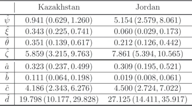
Table 2 shows the estimates of the MP/ztnb model for the parametersa=ψξ

and b = ψξ2 _{of the incidence process N}

t defined in (6) and for the mean c :=

E(Yt|Nt = 1) and variance d := Var(Yt|Nt = 1) of the clump size distribution

defined in (11) and (12). The parameter a is not significantly different in the samples from Kazakhstan and Jordan, suggesting that a sheep gets infected on average every third year. The parameterb is significant larger in the Kazakhstan sample, so that the variance of the infection rates Var(Nt) = at+bt2 is larger for this sample. The difference of the variance of the infection rate in the two

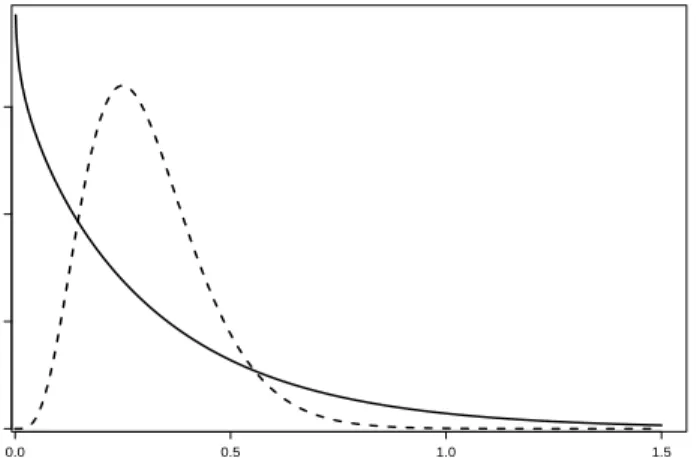
samples is especially pronounced in older sheep since Var(Nt)∼bt2. The result-ing gamma mixture distributions (4) of the infection rate for the two samples are plotted in Figure 1, indicating that in the Kazakhstan sample, the infection rates are more heterogeneous than in the Jordan sample. Table 2 also indicates that the estimated mean and variance for the clump size distribution are not signif-icantly different in the two samples, suggesting that the number of successfully established cysts per infection is similar in the two samples. Thus on average, an infective clump leads to about 4−5 established cysts in the sheep.

[Figure 1 about here.]

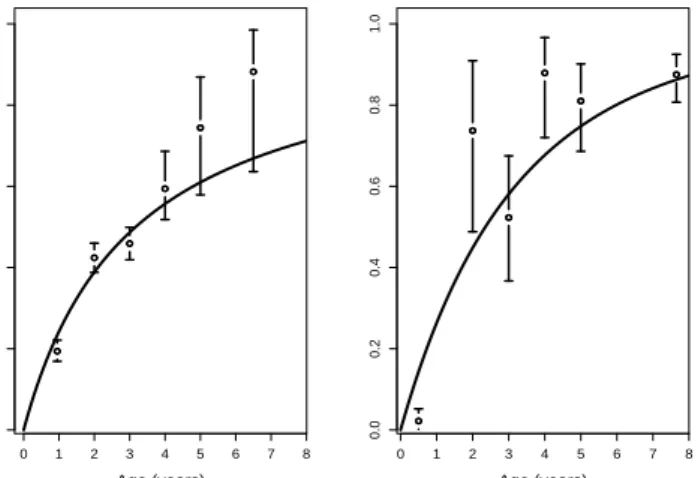
The fitted MP/ztnb model provides estimates for the prevalence of infection as well as for the probability mass function (pmf) of the positive loads. Fig-ure 2 shows the estimated prevalence of infection for the MP/ztnb model for the Kazakhstan and Jordan samples together with the observed prevalences. In both samples, the estimated prevalence of the MP/ztnb explains the observations reasonably well.

[Figure 2 about here.]

The estimated pmf of the MP/ztnb model for the age classes reported in Figure 2 are displayed in Figure 3 for the Kazakhstan and in Figure 4 for the Jordan sample. Given an age class, the fitted pmf are computed as mixture of the pmf’s corresponding to the different ages within the class. The fitted pmf are reasonable in both samples, taking into account the small number of observed positive loads in some of the age classes, especially in the Jordan sample.

[Figure 3 about here.]

4.3

Goodness-of-fit

The goodness-of-fit of the MP/ztnb model is evaluated as follows. Divide the sheep into age classes, and treat the observations in the different classes as i.i.d. data. The classes are specified as in Figure 2. The observed and estimated dis-tributions of cysts are then compared within each age class using an appropriate statistic. Note that, as before, the resulting pmf for an age class is a mixture of the pmf’s corresponding to the different ages within that class.

With the age classes as before, letni1≤i≤6be the number of animals in age class i, and stratify them with respect to load into ci strata. Then two possible goodness-of-fit measures for the distribution of the numbers of cysts within any given age class i are

χ2 := ci X k=1 (mik−E(Mik)) 2 E(Mik) and L:= ci X k=1 ¯ ¯ ¯ ¯ E µ Mik ni ¶ − mik ni ¯ ¯ ¯ ¯ ,

where Mik is a random variable describing the numbers of animals of age class

i having cyst counts in stratum k (1 ≤ k ≤ ci), and mik is the (corresponding) observed count.

The number of strata ci for age class i is chosen to be the maximal number such that the expected number of counts in each stratum is at least 10. The strata in the age classes are computed for the model with parameters fixed by their estimates in Table 2. To generate the reference distribution ofχ2 _{and L, a}

Monte Carlo approach is used, where data sets are generated under the MP/ztnb model. Given the original ages tk (1 ≤ k ≤ n) of the n sheep in the sample, a new cyst burden is attributed to each of them as a realization of the MP/ztnb model witht =tk and the parameters fixed by their estimates given in Table 2.

We then fit the MP/ztnb model to this new data set, and compute with the new estimates the test statistics for each of these sets. We use the same stratification of the age classes as before. The observed values of the two test statistics can then be compared to the reference distributions for each age classi.

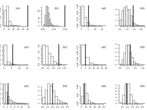
Figures 5 and 6 display the results for the samples from Kazakhstan and Jordan for1000 simulations. For the Kazakhstan sample, the observed values of the test statisticsχ2 _{andL(indicated by a solid line) although consistently large,}

are in reasonable agreement with the simulated distributions for all age strata. For the Jordan sample, the solid line lies well outside the simulated distribution in age class(0,1]. This is for two reasons. First, the observed prevalence in that age class is overestimated by the model (see Figure 2). Secondly, there are only12 positive loads in that class, which are not well described by the model. However, the results in the other age classes suggest that the model fit is reasonable.

The model seems to have some tendency to underestimate the zero load stra-tum and to overestimate the numbers of high cyst counts in the first age class. The opposite tendency can be observed in the age strata 4−6. Since only 4 parameters are used in the model, to fit the distributions of prevalence and cyst burden observed in 6different age classes, a perfect fit can hardly be expected.

[Figure 5 about here.]

[Figure 6 about here.]

5

Conclusion

In this paper, different mechanistic models are used to explain the acquisition of hydatid cysts in sheep, caused by the parasite Echinococcus granulosus. The

models allow one to test the biologically interesting hypotheses of clumped infec-tions, host heterogeneity with respect to infection and aggregation of clump sizes. The experimentally supported assumptions of Echinococcus granulosus cysts in-fections in sheep such as life-long survival of cysts in the host, no replication inside the host, no parasite-induced mortality and no acquired immunity in sheep imply simpler infection dynamics than for example those encountered by [22] and [26], as discussed in the introduction to this paper. Hence our models are straight-forward to fit to the most commonly available data sets, which only contain the ages and cyst burdens of the sheep. The models provide age-dependent estimates for the prevalence of infection and for the probability mass functions of positive cyst burdens in sheep.

The application of the models to two data sets from Kazakhstan and Jordan supports a clumped infection process, with a rate of acquisition of infection which is heterogeneous within the population, and with clump sizes which are aggre-gated. The infection process is described by a compound mixed Poisson process with a zero-truncated negative binomial distribution for the number of cysts per ingested clump. The goodness-of-fit measures indicate that the chosen model describes the given data reasonably well, but not perfectly. The estimates sug-gest a mean infection rate of about0.315 infections per year and a mean clump size of about4.5 cysts, suggesting that on average every third year, a sheep will ingest an infectious clump, each clump leading to approximately4−5established hydatid cysts in the sheep. The results indicate that the observed aggregation in the distribution of cysts among sheep may be the result both of differences between sheep and also of clumped infections.

Our model can be used to investigate how changes in the underlying param-eters may affect the parasite distribution, and thus may be useful in assessing

control programs for Echinococcus granulosus. In particular, it can be used as sub-process for describing infections in the sheep population in a fully stochastic model for the complete life-cycle ofEchinococcus granulosus.

AchnowledgementsThe authors gratefully acknowledge the comments and

suggestions of two referees and the handling editor, that greatly improved the presentation. This work was supported by the Schweizerischer Nationalfonds (SNF), project no. 107726.

References

[1] M. A. Gemmell, J. R. Lawson, M. G. Roberts, Population dynamics in echinococ-cosis and cysticerechinococ-cosis: biological parameters of Echinococcus granulosus in dogs and sheep, Parasitology 92 (1986) 599–620.

[2] P. R. Torgerson, D. H. Williams, M. N. Abo-Shehada, Modelling the prevalence of Echinococcus and Taenia species in small ruminants of different ages in northern Jordan, Vet Parasitol 79 (1998) 35–51.

[3] P. R. Torgerson, B. S. Shaikenov, A. T. Rysmukhambetova, A. E. Ussenbayev, A. M. Abdybekova, K. K. Burtisurnov, Modelling the transmission dynamics of Echinococcus granulosus in sheep and cattle in Kazakhstan, Vet Parasitol 114 (2003b) 143–153.

[4] T. E. Balling, W. Pfeiffer, Frequency distributions of fish parasites in the perch

Perca fluviatilis l. from Lake Constancee, Parasitol Res 83 (1997) 370–373.

[5] C. I. Bliss, R. A. Fisher, Fitting the negative binomial distribution to biological data, Biometrics 9 (1953) 176–200.

[6] C. M. Budke, J. Qiu, P. S. Craig, P. R. Torgerson, Modeling the transmission of Echinococcus granulosus and Echinococcus multilocularis in dogs for a high endemic region of the Tibetan plateau, Int J Parasitol. 35 (2005) 163–170.

[7] C. E. Tanner, M. A. Curtis, T. D. Sole, G. K., The nonrandom, negative binomial distribution of experimental trichinellosis in rabbits, Parasitology 66 (1980) 802– 805.

[8] Z. Q. Zhang, P. R. Chen, K. Wang, X. Y. Wang, Overdispersion of Allothrombium pulvinum larvae (Acari: Trombidiidae) parasitic on Aphis gossypii (Homoptera: Aphididae) in cotton fields, Ecol Entomology 18 (2008) 379–384.

[9] B. Boag, P. B. Topham, R. Webster, Spatial distribution on pasture of infective larvae of the gastro-intestinal nematode parasites of sheep, Int J Parasitol. 19 (1989a) 681–685.

[10] B. Boag, H. H. Kolb, Influence of host age and sex on nematode populations in the wild rabbit (Oryctolagus cuniculus L.), P. Helm. Soc. Wash. 56 (1989b) 116–119. [11] S. W. Pacala, A. P. Dobson, The relation between the number of parasites per host

and host age: population dynamic causes and maximum-likelihood estimation, Parasitology 96 (1988) 197–210.

[12] C. Braga, R. Ximenes, J. Miranda, N. Alexander, Bancroftian filariasis in an en-demic area of Brazil: differences between genders during puberty, Rev. Soc. Bras. Med. Trop. 38 (2005) 224–228.

[13] R. J. Irvine, A. Stien, J. F. Dallas, O. Halvorsen, R. Langvatn, S. D. Albon, Life-history strategies and population dynamics of abomasal nematodes in Svalbard reindeer (Rangifer tarandus platyrhynchus), Parasitol 120 (2000) 297–311.

[14] E. Dietz, D. Boehning, On estimation of the Poisson parameter in zero-modified Poisson models, Comput. Stat. Data Anal. 34 (2000) 441–459.

[15] N. L. Johnson, S. Kotz, Distributions in Statistics: Discrete Distributions, Boston: Houghton Mifflin, 1969.

[16] C. Li, J. Lu, J. Park, K. Kim, P. A. Brinkley, J. P. Peterson, Multivariate zero-inflated Poisson models and their applications, Technometrics 41 (1999) 29–38. [17] A. C. Cohen, An extension of a truncated Poisson distribution, Biometrics 16

(1960) 447–450.

[18] N. Duan, W. G. J. Manning, C. Morris, J. Newhouse, Choosing between the sample selection model and the multi-part model, JBES 2 (1984) 283–289.

[19] C. E. Rose, S. W. Martin, K. A. Wannemuehler, B. D. Plikaytis, On the use of zero-inflated and hurdle models for modeling vaccine adverse event count data, J Biopharm Stat. 16 (2006) 463–481.

[20] A. Nodtvedt, I. Dohoo, J. Sanchez, G. Conboy, L. DesCôteaux, G. Keefe, L. K., J. Campell, The use of negative binomial modelling in a longitudinal study of gastrointestinal parasite burdens in Canadian dairy cows, Can J Vet Res. 66 (2002) 249–257.

[21] P. K. Das, S. Subramanian, A. Manoharan, K. D. Ramaiah, P. Vanamail, B. T. Grenfell, D. A. P. Bundy, E. Michael, Frequency distribution of Wuchereria ban-crofti infection in the vector host in relation to human host: evidence for density dependence, Acta Tropica 60 (1995) 159–165.

[22] J. Herbert, V. Isham, Stochastic host-parasite interaction models, J. Math. Biol. 40 (2000) 343–371.

[23] G. M. Tallis, M. Leyton, Stochastic models of populations of helminthic parasites in the definitive host, Math Biosci 4 (1969) 39–48.

[24] A. D. Barbour, M. Kafetzaki, Modeling the overdispersion of parasite loads, Math Biosci 107 (1991) 249–253.

[25] C. J. Luchsinger, Stochastic models of a parasitic infection, exhibiting three basic reproduction ratios, J Math Biol 42 (2001)(6) 532–554.

[26] B. T. Grenfell, K. Wilson, V. S. Isham, H. E. G. Boyd, K. Dietz, Modelling pat-terns of parasite aggregation in natural populations: trichostrongylid nematode-ruminant interactions as a case study, Parasitology 111(Suppl.) (1995) 135–151. [27] A. Pugliese, R. Rosa, M. L. Damaggio, Analysis of a model for macroparasitic

infection with variable aggregation and clumped infections, J Math Biol 36 (1998) 419–447.

[28] R. C. A. Thompson, A. J. Lymbery, The biology of Echinococcus and hydatid disease, London: George Allen and Unwin, 1986.

[29] B. Todorov, V. Boeva, Human echinococcosis in Bulgaria: a comparative epidemi-ologiocal analysis, Bulletin WHO 77 (1999) 110–118.

[30] P. R. Torgerson, B. Shaikenov, K. K. Baitursinov, A. M. Abdybekova, The emerg-ing epidemic of echinococcosis in Kazakhstan, Trans R Soc Trop Med Hyg 96 (2002) 124–128.

[31] P. R. Torgerson, B. Oguljahan, M. E. Muminov, R. R. Karaeva, O. T. Kuttubaev, M. Aminjanov, B. Shaikenov, Present situation of cystic echinococcosis in Central Asia, Parasitol Int. 55 (2006) 207–212.

[32] J. Eckert, P. Deplazes, Biological, epidemiological and clinical aspects of Echinococcosis, a zoonosis of increasing concern, Clin Microbiol Rev. 17 (2004) 107–135.

[33] D. R. Cox, V. Isham, Point Processes, New York: Chapman and Hall, 2 edition, 1980.

[34] D. J. Daley, D. Vere-Jones, An introduction to the theory of point processes, New York: Springer, 2 edition, 1988.

[35] A. F. Karr, Point processes and their statistical inference, Marcel Dekker, Inc., 2 edition, 1991.

[36] M. A. Gemmell, Hydatid disease in Australia, III. Observations on the incidence and geographical distribution of hydatidiasis in sheep in New South Wales, Aust Vet J 34 (1958) 269–280.

[37] M. G. Roberts, J. R. Lawson, M. A. Gemmell, Population dynamics in echinococ-cosis and cysticerechinococ-cosis: Mathematical model of the life-cycle of Echninococcus granulosus, Parasitology 92 (1986) 621–641.

[38] P. R. Torgerson, D. D. Heath, Transmission dynamics and control options for cystic echinococcosis, Parasitology 127 (2003d) 143–158.

[39] J. L. Teugels, P. Vynckier, The structure distribution in a mixed poisson process, JAMSA 9 (1996)(4) 489–496.

[40] B. Buchmann, R. Grübel, Decompounding Poisson random sums: Recursively truncated estimates in the discrete case, Ann. Statist. 31 (2003) 1054–1074. [41] H. R. Panjer, Recursive evaluation of a family of compound distributions, ASTIN

Bulletin 12 (1981) 22–26.

[42] J. Springael, I. van Nieuwenhuyse, On the sum of independent zero-truncated Pois-son random variables, Research paper UA, Faculty of Applied Economics (2006).

[43] T. Cacoullos, C. Charalambides, On minimum variance unbiased estimation for truncated binomial and negative binomial distributions, Ann Inst Stat Math. 27 (1975) 235–244.

[44] S. G. Self, K. Y. Liang, Asymptotic properties of maximum likelihood estimators and likelihood ratio tests under nonstandard conditions, JASA 4 (1987) 605–610.

Figures

Figure 1: Estimated gamma density function (4) of the infection rate in the inci-dence process for the samples from Kazakhstan (solid line) and Jordan (dashed line).

0.0 0.2 0.4 0.6 0.8 1.0 Kazakhstan Age (years) Prevalence 0 1 2 3 4 5 6 7 8 0.0 0.2 0.4 0.6 0.8 1.0 Jordan Age (years) 0 1 2 3 4 5 6 7 8

Figure 2: Fitted prevalence curvesqˆ(t) = 1−1/(tξˆ+ 1)ψˆ _{(with ψ}ˆ _{and ξ}ˆ_{given in} Table 2) for the MP/ztnb model for the samples from Kazakhstan and Jordan, together with the observed prevalences and their 95% confidence intervals. The observed prevalences are computed for the age classes (0,1], (1,2], (2,3], (3,4], (4,5],5+, where5+ summarizes all sheep older than 5years. For the age classes 1− 4, the majority of the observed ages coincide with the end points of the interval. The prevalences are plotted at the means of the ages of the animals in the corresponding classes.

13579 12 15 18 21 24 27 30 Mass 0.00 0.05 0.10 0.15 0.20 0.25 (a) 147 11 15 19 23 27 31 35 39 43 0.00 0.05 0.10 0.15 0.20 0.25 (b) 1 4 7 1115 1923 2731 3539 0.00 0.05 0.10 0.15 0.20 0.25 (c) 147 11 15 19 23 27 31 35 39 43 Cyst load Mass 0.00 0.05 0.10 0.15 (d) 147 11 15 19 23 27 31 35 39 43 Cyst load 0.00 0.05 0.10 0.15 (e) 1 3 5 7 9 1215 182124 2730 Cyst load 0.00 0.05 0.10 0.15 (f)

Figure 3: Estimated probability mass functions of the MP/ztnb model for the positive loads of the Kazakhstan sample for the age classes (a)(0,1], (b)(1,2], (c) (2,3], (d)(3,4], (e)(4,5], (f)5+, together with a histogram of the corresponding observed quantities. The class sizes are185,315,282,84,29and 15. For a better presentation of the results, the following points are not plotted in the histograms: 64(with corresponding mass0.003) in age class(1,2],47and57(mass0.119each) in age class(3,4]and 56(mass 0.034) in age class(4,5].

13579 12 15 18 21 24 27 30 Mass 0.0 0.1 0.2 0.3 0.4 (a) 1 4 7 10 14 18 22 26 30 34 38 0.0 0.1 0.2 0.3 0.4 (b) 1 4 7 10 14 18 22 26 30 34 38 0.0 0.1 0.2 0.3 0.4 (c) 1 4 7 11 15 19 2327 31 35 39 Cyst load Mass 0.00 0.05 0.10 0.15 (d) 147 11 15 19 23 27 31 35 39 43 Cyst load 0.00 0.05 0.10 0.15 (e) 147 11 15 19 23 27 31 35 39 43 Cyst load 0.00 0.05 0.10 0.15 (f)

Figure 4: Estimated probability mass functions of the MP/ztnb model for the positive loads of the Jordan sample for the age classes (a) (0,1], (b) (1,2], (c) (2,3], (d)(3,4], (e)(4,5], (f)5+, together with a histogram of the corresponding observed quantities. The class sizes are12,14,23,29, 47and 119. For an better presentation of the results, the following points are not plotted in the histograms: 52and63(mass0.021 each) in age class(4,5], and57(mass0.008) and two loads of 80(combined mass 0.016) in age class 5+.

Density 0 10 20 30 40 0.00 0.04 0.08 (a1) 0.02 0.06 0.10 0 5 10 20 (b1) 0 5 10 15 20 0.00 0.04 0.08 0.12 (a4) 0.00 0.10 0.20 0.30 0 2 4 6 (b4) Density 0 10 20 30 40 0.00 0.04 0.08 (a2) 0.04 0.08 0.12 0 5 10 15 20 25 (b2) 0 2 4 6 8 10 12 0.00 0.10 0.20 0.30 (a5) 0.0 0.2 0.4 0 1 2 3 4 _(b5) χ2 _statistic Density 0 10 20 30 40 0.00 0.02 0.04 0.06 (a3) L statistic 0.06 0.10 0.14 0.18 0 5 10 15 (b3) χ2 _statistic 0 5 10 15 0.0 0.1 0.2 0.3 0.4 (a6) L statistic 0.0 0.2 0.4 0.6 0.8 1.0 0.0 1.0 2.0 3.0 (b6)

Figure 5: Goodness-of-fit of the MP/ztnb model in the Kazakhstan sample. The observed values of the test statistics (solid lines)χ2 _{((a1)-(a8)) andL((b1)-(b8))}

are plotted with the corresponding simulated distributions under the MP/ztnb model with parameters fixed with its estimates in Table 2 for the age classes (x1) (0,1], (x2) (1,2], (x3) (2,3](x4) (3,4], (x5) (4,5]and (x6) 5+, with x=a,b.

Density 0 10 20 30 40 50 0.00 0.04 0.08 (a1) 0.00 0.10 0.20 0 5 10 20 (b1) 0 5 10 15 0.00 0.10 0.20 0.30 (a4) 0.0 0.2 0.4 0.6 0 1 2 3 (b4) Density 0 5 10 15 0.0 0.1 0.2 0.3 0.4 _(a2) 0.0 0.2 0.4 0.6 0.8 0.0 1.0 2.0 3.0 (b2) 0 5 10 15 20 25 30 0.00 0.04 0.08 0.12 (a5) 0.0 0.2 0.4 0.6 0 1 2 3 4 5 (b5) χ2 _statistic Density 0 2 4 6 8 10 14 0.0 0.1 0.2 0.3 0.4 _(a3) L statistic 0.0 0.1 0.2 0.3 0.4 0.5 0 1 2 3 4 (b3) χ2 _statistic 0 10 20 30 40 50 0.00 0.04 0.08 (a6) L statistic 0.1 0.2 0.3 0.4 0.5 0 1 2 3 4 5 6 _(b6)

Figure 6: Goodness-of-fit of the MP/ztnb model in the Jordan sample, analo-gously to Figure 5.

Tables

Table 1: Log-likelihood values for the models fitted to the Kazakhstan and Jordan samples, together with the number of parameters in the models.

Model Kazakhstan Jordan Parameters P/1 −10648.570 −2643.109 1 MP/1 −4230.321 −1133.255 2 P/ztP −4647.557 −1161.142 2 P/ztnb −4179.769 −1018.524 3 MP/ztP −4180.413 −1079.412 3 MP/ztnb −4160.347 −1016.665 4

Table 2: Maximum likelihood estimates for the parameters and key quantities of the MP/ztnb model for the Kazakhstan and Jordan samples, together with 95% confidence intervals computed by the bootstrap percentile method. The parameters a = ψξ and b = ψξ2 _{of the incidence process N}

t are defined in (6), so that E(Nt) = at and Var(Nt) = at+bt

2_{. The mean c :=}

E(Yt|Nt = 1) and

variance d := Var(Yt|Nt = 1) of the clump size distribution are defined in (11) and (12) respectively. Kazakhstan Jordan ˆ ψ 0.941 (0.629,1.260) 5.154 (2.579,8.061) ˆ ξ 0.343 (0.225,0.741) 0.060 (0.029,0.173) ˆ θ 0.351 (0.139,0.617) 0.212 (0.126,0.442) ˆ ζ 5.859 (3.215,9.763) 7.861 (5.394,10.565) ˆ a 0.323 (0.237,0.499) 0.309 (0.195,0.521) ˆ_{b 0.111 (0.064,0.198) 0.019 (0.008,0.061)} ˆ c 4.186 (2.343,6.276) 4.500 (2.724,7.022) ˆ d 19.798 (10.177,29.828) 27.125 (14.411,35.917)