2017
Graphical discovery in stochastic actor-oriented
models for social network analysis
Samantha Carroll Tyner
Iowa State UniversityFollow this and additional works at:
https://lib.dr.iastate.edu/etd
Part of the
Statistics and Probability Commons
This Dissertation is brought to you for free and open access by the Iowa State University Capstones, Theses and Dissertations at Iowa State University Digital Repository. It has been accepted for inclusion in Graduate Theses and Dissertations by an authorized administrator of Iowa State University Digital Repository. For more information, please [email protected].
Recommended Citation
Tyner, Samantha Carroll, "Graphical discovery in stochastic actor-oriented models for social network analysis" (2017).Graduate Theses and Dissertations. 16751.
models for social network analysis
by
Samantha Carroll Tyner
A dissertation submitted to the graduate faculty in partial fulfillment of the requirements for the degree of
DOCTOR OF PHILOSOPHY
Major: Statistics
Program of Study Committee: Heike Hofmann, Major Professor
Alicia Carriquiry Dianne Cook
Olga Chyzh Cindy Yu
The student author, whose presentation of the scholarship herein was approved by the program of study committee, is solely responsible for the content of this dissertation. The Graduate College will ensure this dissertation is globally accessible and will not permit alterations after a degree is
conferred.
Iowa State University Ames, Iowa
2017
DEDICATION
I would like to dedicate this thesis to the all the amazing women in my life, who have guided and encouraged me on my academic journey. Thank you.
Special thanks to Dr. Lara Pudwell, without whom I would have never even considered going to graduate school; Dr. Taddy Kalas, merci pour votre passion et votre intr´epidit´e; my sisters, Jordan, Makenna, Cate, and Jenna; my mom, Cathy, and my grandma, Nancy. Thanks for the brains, Grandma. I wish you could be with me to celebrate.
TABLE OF CONTENTS
Page
LIST OF TABLES . . . vi
LIST OF FIGURES . . . viii
ACKNOWLEDGEMENTS . . . xv
ABSTRACT . . . xvi
CHAPTER 1. LITERATURE REVIEW . . . 1
1.1 Statistical Models for Social Networks . . . 2
1.1.1 Basic Network Terminology and Notation . . . 2
1.1.2 Static Network Models . . . 3
1.1.3 Dynamic Network Models . . . 5
1.1.4 Stochastic Actor-Oriented Models for Longitudinal Social Networks. . . 8
1.2 Network Visualization . . . 15
1.2.1 Layout Algorithms . . . 15
1.2.2 R Packages . . . 18
1.2.3 The Importance of theggplot2 Package . . . 19
1.3 What is Visual Inference? . . . 20
1.3.1 A Formal Definition and Construction . . . 21
1.3.2 Applications of Visual Inference . . . 23
1.4 Summary . . . 24
CHAPTER 2. STOCHASTIC ACTOR-ORIENTED MODELS: REMOVING THE BLIND-FOLD . . . 25
2.2 Networks and their Visualizations . . . 27
2.2.1 Introduction to Network Structures . . . 27
2.2.2 Visualizing Network Data . . . 28
2.3 Stochastic Actor-Oriented Models for Longitudinal Social Networks . . . 31
2.3.1 Definitions, Terminology, and Notation . . . 31
2.3.2 Fitting Models to Data . . . 38
2.3.3 Model Goodness-of-Fit . . . 39
2.3.4 Example Data . . . 40
2.4 Model Visualizations . . . 43
2.4.1 The Models . . . 44
2.4.2 View the model in the data space . . . 45
2.4.3 Visualizing collections of models . . . 49
2.4.4 Explore algorithms, not just end result . . . 54
2.5 Discussion . . . 59
CHAPTER 3. VISUAL INFERENCE FOR SIGNIFICANCE AND GOODNESS-OF-FIT TESTING OF STOCHASTIC ACTOR-ORIENTED MODELS . . . 74
3.1 Introduction . . . 74
3.2 Visual Inference . . . 75
3.3 Stochastic Actor-Oriented Models . . . 76
3.3.1 Rate Function . . . 77 3.3.2 Objective Function . . . 78 3.3.3 Example Data . . . 79 3.3.4 Models of Interest . . . 81 3.4 Experiment Set-Up . . . 84 3.4.1 Significance Testing . . . 85 3.4.2 Goodness-of-Fit . . . 86 3.4.3 Visual Power . . . 86
3.5 Experiment Results . . . 89
3.5.1 Significance Testing . . . 89
3.5.2 Goodness-of-Fit Testing . . . 91
3.5.3 Visual Power . . . 95
3.6 Discussion . . . 98
CHAPTER 4. DRAWING NETWORK DATA WITH THERPACKAGE ggplot2 . . . 115
4.1 Brief introduction to networks . . . 118
4.2 Three implementations of network visualizations . . . 120
4.2.1 ggnet2 . . . 121 4.2.2 geomnet . . . 123 4.2.3 ggnetwork . . . 128 4.3 Examples . . . 131 4.3.1 Blood donation . . . 131 4.3.2 Email network . . . 135
4.3.3 ggplot2theme elements . . . 142
4.3.4 College football . . . 143
4.3.5 Southern women . . . 146
4.3.6 Bike sharing in Washington D.C. . . 147
4.4 Some considerations of speed . . . 152
4.5 Summary and discussion . . . 154
CHAPTER 5. SUMMARY AND DISCUSSION . . . 173
BIBLIOGRAPHY . . . 175
LIST OF TABLES
Page
Table 1.1 Some propensity functions to describe the network dynamics in CTMC models. 7
Table 1.2 Some of the possible effects to be included in the stochastic actor-oriented models inRSiena. There are many more possible effects, but we only con-sider a select few here. For a complete list, see the RSiena manual (Ripley et al 2016). . . 12
Table 2.1 Some of the possible effects to be included in the stochastic actor-oriented models in RSiena. There are many more possible effects, but we only con-sider a select few here. For a complete list, see the RSienamanual (Ripley et al. 2017). . . 35
Table 2.2 The means (standard deviations) of parameter values estimated from re-peated fittings ofM1, M2, M3 to the small friendship network and the sen-ate collaboration network. Each model was fit 1,000 times to the friend data, while each model was fit 100 times to the senate data. . . 52
Table 3.1 The additional effects we used in the SAOMs fit to the senate data. * - simbij = maxhk|bh−bk|−|bi−bj|
maxhk|bh−bk| is the similarity score between two senators based on the number of bills authored, andsimb = n(n1−1)P
i6=jsimbij is the
average bill similarity score between any two senators. . . 83
Table 3.2 The final estimates from repeated estimation of our models of interest. When simulating from these models, these are the estimates that we will use unless otherwise stated. . . 84
Table 3.3 All conditions used for the MTurk experiment. For parameters β1, β2, β3,
and β5 M1 served as null model. For β4 and β6, null model M1 and the
alternative model switch roles in the reversed lineups, i.e. five plots show data simluated from the laternative model and only one plot shows data from M1. . . 88
Table 3.4 Experiment results for the two parameters for which we performed signifi-cance tests. There were three lineups for each parameter, so there are three results for each plot. . . 90
Table 3.5 An overview of the results from the 12 goodness-of-fit lineup tests. . . 93
Table 3.6 Summary of the results from fitting the model given in Equation3.11. Sig-nificance levels: * - <0.10; ** -<0.05;† - <0.01;‡ - <0.001 . . . 97
LIST OF FIGURES
Page
Figure 1.1 The same random network plotted with the default options in igraph(at left) and network(at right) . . . 20
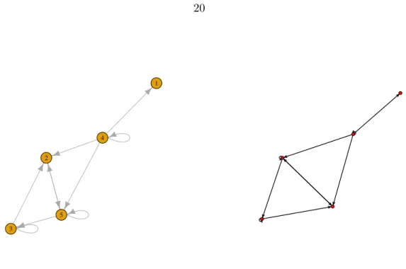
Figure 2.1 On the left, a node-link diagram of our directed toy network, with nodes placed using the Kamada-Kawai algorithm . . . 29
Figure 2.2 The probability distribution function for the type 1 extreme value distribu-tion, also known as the log-Weibull or Gumbel distribution with location parameterµ= 0 and scale parameter σ= 0 . . . 36
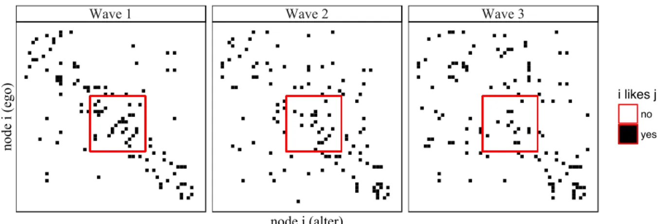
Figure 2.3 A visualization of the adjacency matrices of the three waves of network observations in the “Teenage Friends and Lifestyle Study” data . . . 40
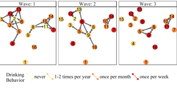
Figure 2.4 The smaller friendship network data we will be modelling throughout the paper . . . 41
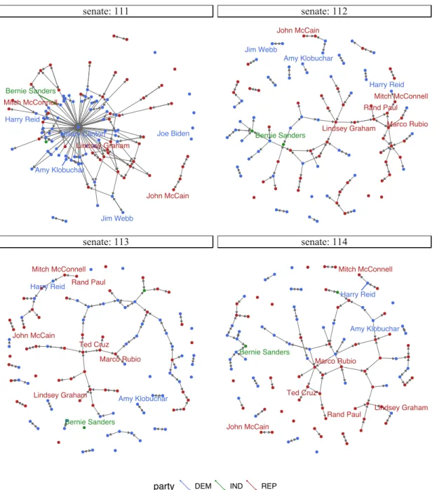
Figure 2.5 The collaboration network in the four senates during the Obama years, 2009-2016 . . . 61
Figure 2.7 Realization of a jumping transitive triplet, where i is the focal actor, j is the target actor, and h is the intermediary. The group of the actors is represented by the shape of the node. . . 62
Figure 2.8 Doubly achieved distance between actorsiand k. . . 62
Figure 2.9 The additional network effects included in our models fit to the friends data. On the left, a jumping transitive triplet (JTT). On the right, a doubly achieved distance between iandk. . . 62
Figure 2.10 The 111th Senate at two discrete time points . . . 62
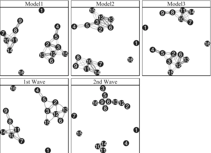
Figure 2.12 A small lineup of node-link diagrams showing the second wave of our small friendship network among five networks simulated from model M1. . . 63
Figure 2.13 Significant effects for the two data sets, at a significance level of 0.10 or lower as calculated by the Wald-type test available in the SIENA software . 64
Figure 2.14 The node-link diagrams from the three ”average” networks that we calcu-lated are in the top row, and the true wave 1 and wave 2 data are shown in the bottom row above . . . 65
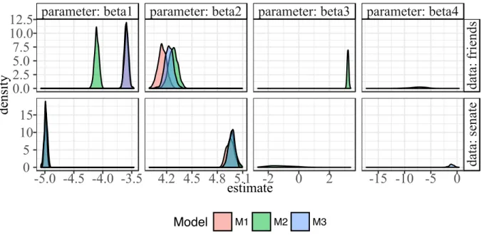
Figure 2.15 Density plots of the repeated estimates from fitting models M1, M2, and M3 to the friendship and senate example data . . . 66
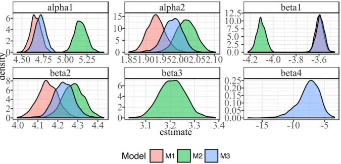
Figure 2.16 Distribution of fitted parameter values for our three SAOMs . . . 67
Figure 2.17 A matrix of plots demonstrating the strong correlations between parameter estimate in our SAOMs . . . 68
Figure 2.18 A selection of images in the microstep animation . . . 69
Figure 2.19 On the left, the starting friendship network represented in adjacency matrix form, ordered by vertex id . . . 69
Figure 2.20 A selection of frames from the adjacency matrix visualization animation for one series of microsteps . . . 70
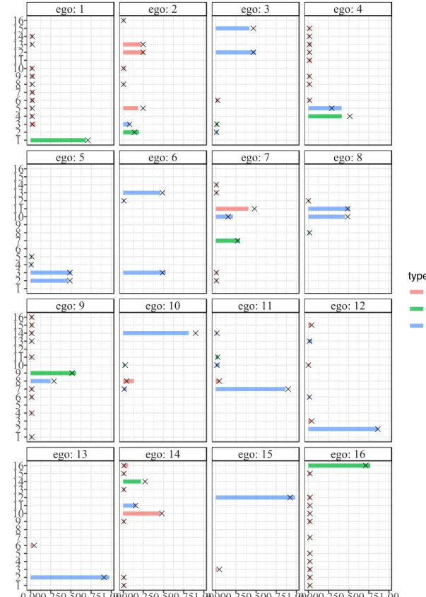
Figure 2.21 Each panel shows the theoretical (as lines) and empirical (as points) prob-abilities of the chosen ego node changing its tie to each of the other nodes . 71
Figure 2.22 A heatmap showing the empirical transition probabilities for the first mi-crostep in 1,000 simulations . . . 72
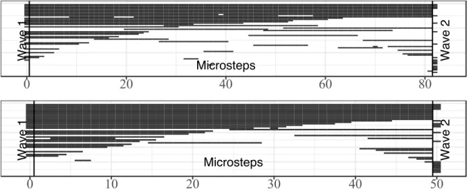
Figure 2.23 Two simulations (out of 1,000) of the microstep process from wave 1 to wave 2 72
Figure 2.24 Visualizing all microsteps taken in 1,000 simulations from the model M1 . . 73
Figure 3.1 The four senate collaboration networks that we use as our example data to visually assess the SAOM effects . . . 100
Figure 3.2 We removed Hillary Clinton’s ties from the network because she had abnor-mally high collaboration with senators during the time she was in the 111th senate and before she left office to become Secretary of State . . . 101
Figure 3.3 A screen shot of the web application we created to design our lineup experi-ment. More details about this application are given in Section3.4.3. In the lineup, M5 is the alternative model withβ5 set to twice its estimated value
given in Table3.2. One plot simulated from this model is placed at random among five observations simulated from the null model, M1. Participants of the study are asked to identify the most different plot. . . 102
Figure 3.4 We hypothesize that as the parameter value of interest increases in absolute value, more viewers of the lineup will pick the alternative data out of a lineup. Note that the significance test we construct in Section 3.4.1 is just one point on the line below, represented by the vertical dotted line labeled
ˆ
β. The easy, medium, and hard lines represent how we determined which values of the parameters to show to our participants, and the horizontal dotted line shows the type-I error for one viewer of a lineup of size 6. . . 102
Figure 3.5 The lineup which caused a rejection of the null hypothesis thatβ3 = 0 . . . 103
Figure 3.6 One of the lineups which failed to reject the null hypothesis thatβ3 = 0 . . 104
Figure 3.7 An example of what a goodness-of-fit plot fromRSienalooks like . . . 105
Figure 3.8 The goodness-of-fit lineup that failed to reject the null hypothesis . . . 106
Figure 3.9 One repitition of a goodness-of-fit lineup testing modle M7 . . . 107
Figure 3.11 Predictions from our generalized linear mixed effects model given in Equa-tion efeq:glmm. The lines show the expected probability of detecting the alternative data in a lineup of size 6 for new observers of new lineups is plot-ted on the y-axis, and the size of the parameter of interest is on thex-axis. The proportions detected by our Turk participants for each lineup group are shown by the points, with the probability of picking out the data plot at random shown by a horizontal line at 1/6. The lineup marked as “outlier” was removed from modeling. The panel for the reciprocity parameter,β2 is
also presented in Figure 3.12in more detail. . . 109
Figure 3.12 The top middle panel of Figure3.11 expanded to show greater detail. The square root of the parameter value is shown on thex-axis. For this parame-ter, as its value approaches zero, the probability of identifying the alternate data model decreases, then increases, which is noticeably different from the pattern exhibited by the others. Again, a horizontal line is drawn at 1/6, the chance of selecting the data plot at random. . . 110
Figure 3.13 The bottom middle panel of Figure 3.11 expanded to show greater detail. The parameter value is shown on the x-axis. This parameter most closely follows our hypothesis shown in Figure3.4. However, the result is not sym-metric. According to the model, people will detect the effect at lower values and with greater frequency as the value increases when it is positive instead of negative. . . 111
Figure 3.14 The bottom left panel of Figure 3.11expanded to show greater detail. The parameter value is shown on the x-axis. The “reverse” lineup has a much flatter slope than the “regular” lineup, which means the participants had a harder time detecting a more simple M1 structure among many more complex M4 structures. Reversing the lineup scenario was not symmetric as we hypothesized. . . 112
Figure 3.15 In our experiment, 52.8% of viewers of this plot selected the plot from the alternative model, M4. The “reverse” of this lineup is given in Figure 3.16, where 41.4% of viewers selected the plot from the alternative model, M1.
Here, the alternative plot is√25−3. . . 113
Figure 3.16 In our experiment, 41.4% of viewers of this plot selected the plot from the alternative model, M1. The “reverse” of this lineup is given in Figure 3.15, where 52.8% of viewers selected the plot from the alternative model, M1. Here, the alternative plot is√25−1. . . 114
Figure 4.1 Graph of the characters in the show Mad Men who are linked by a romantic relationship. . . 119
Figure 4.2 The code required to generate Figure 4.1using the ggnet2 function in the ggallypackage. . . 121
Figure 4.3 The code required to generate Figure4.1using thegeom netfunction in the geomnetpackage. . . 124
Figure 4.4 The code required to generate Figure4.1 using theggnetwork package. . . . 129
Figure 4.6 ggnet2 . . . 134
Figure 4.7 geomnet . . . 134
Figure 4.8 ggnetwork . . . 134
Figure 4.9 Network of blood donation possibilities in humans by ABO and RhD blood types. . . 134
Figure 4.11 ggnet2 . . . 159
Figure 4.12 geomnet . . . 159
Figure 4.13 Email network within a company over a two week period. . . 159
Figure 4.14 ggnetwork . . . 160
Figure 4.15 (continued) Email network within a company over a two week period. . . 160
Figure 4.17 ggnet2 . . . 161
Figure 4.19 The same email network as in Figure4.13 faceted by day of the week. . . . 161
Figure 4.20 ggnetwork . . . 162
Figure 4.21 (continued) The same email network as in Figure4.13faceted by day of the week. . . 162
Figure 4.23 ggnet2 . . . 163
Figure 4.24 geomnet . . . 163
Figure 4.25 Inheritance structure of ggplot2 theme elements. This is a recreation of the graph found athttp://docs.ggplot2.org/current/theme.html. . . . 163
Figure 4.26 ggnet2 . . . 164
Figure 4.27 (continued) Inheritance structure of ggplot2 theme elements. This is a recreation of the graph found athttp://docs.ggplot2.org/current/theme. html. . . 164
Figure 4.29 ggnet2 . . . 165
Figure 4.30 geomnet . . . 166
Figure 4.31 ggnetwork . . . 166
Figure 4.32 (continued) The network of regular season Division I college football games in the season of fall 2000. The vertices and their labels are colored by conference. . . 166
Figure 4.34 ggnet2 . . . 167
Figure 4.35 Graph of the Southern women data. Women are represented as orange triangles, events as green circles. . . 167
Figure 4.36 geomnet . . . 168
Figure 4.37 ggnetwork . . . 168
Figure 4.38 Graph of the Southern women data. Women are represented as orange triangles, events as green circles. . . 168
Figure 4.40 geographic map . . . 169
Figure 4.42 ggnet2 . . . 169
Figure 4.43 ggnetwork . . . 169
Figure 4.44 Network of bike trips using a geographically true representation(top left) overlaid on a satellite map, a Kamada-Kawai layout ingeomnet(top right), a Fruchterman-Reingold layout inggnet2(bottom left) andggnetwork (bot-tom right). Metro stations are shown in orange. In both the Kamada-Kawai and the Fruchterman-Reingold layouts, metro stations take a much more central position than in the geographically true representation. . . 169
Figure 4.45 Protein-protein interaction network inS. cerevisiae. A Fruchterman-Reingold algorithm allowed to run for 50,000 iterations produced the coordinates for the nodes. . . 170
Figure 4.46 Comparison of the times needed for calculating and rendering the previously discussed protein interaction network in the threeggplot2 approaches and the standard plotting routines of the network and igraph packages based on 100 evaluations each. . . 171
Figure 4.47 Plotting times of random undirected networks of different sizes under each of the available visualization approaches using their default settings. Note that each panel is scaled independently to highlight relative differences in the visualization approaches rather than speed of different hardware. . . . 172
ACKNOWLEDGEMENTS
I would like to take this opportunity to express my thanks to those who helped me with various aspects of conducting research and the writing of this dissertation.
First and foremost, Dr. Heike Hofmann for her guidance, patience, encouragement, excitement, and support throughout this research and the writing of this thesis. Her insights and words of encouragement and wisdom have often inspired me and gave me confidence in the work when I couldn’t muster it for myself. I would also like to thank my committee members for their efforts and contributions to this work: Drs. Alicia Carriquiry, Dianne Cook, Cindy Yu, and extra thanks to Dr. Olga Chyzh for introducing Dr. Hofmann and I to these incredibly memorable stochastic actor-oriented models.
I would additionally like to thank Dr. Bruce Rogers for planting the network bug in my brain, Dr. Eric Hare for his computational assistance, and Dr. Margaret Johnson for her emotional assistance. I couldn’t have done this without you.
ABSTRACT
This work presented in this thesis combines statistical models for social networks and network visualization in new and exciting ways. In Chapter 1, a thorough review of the literature in the topics of statistical network models and network visualization is presented. In Chapter 2, we focus in on one type of model for dynamic social networks: the stochastic actor-oriented models (SAOMs), introduced by Snijders (1996). Unlike other network models, SAOMs are not very well understood, so we use model visualization techniques inspired by those introduced in Wickham et al (2015) in order to make the models a little less murky. The SAOMs are a prime example of a set of models that can benefit greatly from application of model visualization, and with the help of static and dynamic visualizations, we bring the hidden model fitting processes into the foreground, eventually leading to a better understanding and higher accessibility of stochastic actor-oriented models for social network analysts. In Chapter 3, we further explore the SAOMs using the visual inference methodology of Buja et al. (2009). We construct significance tests of model parameters, goodness-of-fit tests, and power calculations for the objective function parameters in SAOMs using visual inference. In this way, we can explore complex network data more completely than traditional significance and goodness-of-fit methods that rely on one-dimensional derived features of networks do. In Chapter 4, we present an R package for drawing networks using the popular grammar of graphics R plotting paradigm, ggplot2 (Wickham 2016). We close with a discussion of the limitations of the work and directions for the future in Chapter 5.
CHAPTER 1. LITERATURE REVIEW
Social networks have been studied for decades, beginning with a few foundational works, the most well known of which is the 1967 study, “The Small World Problem” by Stanley Milgram (Goldenberg et al., 2010). But in recent years, the study of social networks has grown wildly in popularity due to an increase in the availability of and easy of access to social network data. The digital revolution has led to the creation of social media, linking people from all over the world in a way we never have been before. Now that platforms like Facebook, Twitter, and LinkedIn permeate our world, just about everyone knows what social networks are. In academic circles, collaboration networks are a type of social network that have been extensively studied and can even be a point of pride, like a mathematician’s Erd¨os number (Grossman, 2016). Social networks are a rich source of knowledge, but the data format does not fit easily within traditional data collection paradigms. Traditionally, data collection involves a set of units of the same, or at least similar, kind, on which observations are made. The storage of traditional data is simple and organized: rows contain variable values collected from units. These units can be people, plants, animals, stocks, objects, fields, and anything else under the sun, but one social network consits of many units, yet on the whole is just one observation. When observing a social network, one observes the possibly very numerous actors (also referred to as vertices or nodes) and the relationships (also referred to as edges or ties) between those actors. One can also collect information on the nodes and the edges separately, such as the age or gender of people and the length of their relationship or how strong it is in a friendship network. Thus, information on the entire network is more difficult to store than traditional data with which statisticians usually work.
This apparent difficulty has not stopped researchers in many different fields from studying social and other types of networks. Sociologists work with human relationship networks of all kinds imaginable, biologists work with protein-protein interaction networks, neurologists use fMRI scans
to study biologic neural networks, and the list goes on. These disciplines worked separately for many years, each developing their own measures, softwares, and theories about the fundamental properties of networks. And although statisticians were comparatively late to the party, many statistical models exist for network analysis. Beginning with the classic Erd¨os-R´enyi random graph model and varying in structure, complexity, and application to include longitudinal network data, such as continuous time markov chain models (Goldenberg et al., 2010). The many varying models that exist just for social network analysis are impressive, but I focus my research on one type of continuous time markov chain (CTMC) models, called Stochastic Actor-Oriented Models (SAOMs). A full introduction to the various models that exist for social network analysis is presented in Section
1.1, and a full introduction to the structure and theory of SAOMs is presented in Section 1.1.4.
1.1 Statistical Models for Social Networks
The literature on statistical models for networks is extensive. In their thorough “Survey of Statistical Models”, Goldenberg et al. (2010) separate these models into two primary classes: static and dynamic. I discuss the several types of models as they relate to stochastic, actor-oriented models, the models of my primary focus, in each of these two categories after a brief introductory section on general network terminology and notation.
1.1.1 Basic Network Terminology and Notation
Formally, a network is defined by a collection of nodes, also referred to as vertices or actors, and the set of ties, also referred to as edges or relationships, between them. Let x denote a network. The network’s collection of nodes, its nodeset, is writtenN, and its collection of edges, its edgeset, is written. E. Typically, the nodes are numbered so that N ={1,2, . . . , n}, where n is the total number of nodes in the network. The edgeset is usually described as a set of pairs, written as xij
or i j or (i, j), where i 6= j ∈ N. In an undirected network, the ordering of i and j does not matter: there is no parent-child relationship, to use a term from graph theory, just a connection of some kind. In a directed graph, however, the order does matter: the tie xij is not equivalent
to the tiexji. In a simple, undirected graph, the number of possible edges is n2
, while in simple, directed graphs it isn(n−1), assuming no self-loops (also called self-ties or simply loops) and only allowing for at most one edge between any two nodes.
In statistical network analysis, an observed network is written as x, while X denotes an unob-served network being treated as a random variable. I assume binary network ties throughout: if the edge between nodes i and j is present, xij = 1, whereasxij = 0 if the edge is not present. If
x is undirected, then xij =xji∀i6=j∈ N. If x is directed, thenxij may equal xji, but this is not
required and should not be assumed. Note that the definition of binary edge variables makes the assumption that edges are unweighted and that their cannot be more than one edge between two nodes. It is possible for networks to have weighted edges or multiple ties between nodes, but the models I discuss here, including the stochastic actor-oriented models that are my primary focus, are all for unweighted networks.
A networkx can also be expressed as ann×nmatrix of 0s and 1s called the adjacency matrix, denoted A. The ijth entry of this matrix, aij is 1 if there is an edge between nodes iand j and 0
otherwise. The diagonal entries of this matrix, aii are structurally 0, as self-ties or self-loops are
not allowed as mentioned above.
1.1.2 Static Network Models
The Erd¨os-R´enyi random graph model is widely regarded as the first random graph model (Goldenberg et al., 2010). This model, first introduced in Erd¨os and R´enyi (Erd¨os and R´enyi, 1959), describes random, undirected networks. Edges xij are selected at random from all possible
edges. The parameter in this model isp, the probability that an edge exists between any two nodes in the network. The number of edges in the network, e=P
i<jxij, has likelihood
f(e|p, n) =pe(1−p)(n2)−e.
The properties and asymptotic behavior of this network model are well-established (Goldenberg et al., 2010). Nodes in networks generated using this model all have about the same degree, or number of incident edges, which, in practice, is a very unrealistic property for a network to have. As
such, many other models have been devised over the years as a way to better capture the network creation process underlying real-world networks.
In order to better model real-world networks, the exponential random graph family of models (ERGMs) was developed. These are also referred to asp∗models after the first use of the exponential family form in thep1model for directed networks of Holland and Leinhardt (Holland and Leinhardt,
1981). This class of models uses structural properties of the network as sufficient statistics in the likelihood. The properties used are different for directed and undirected graphs. Some statistics used for directed networks are the outdegree of the nodes, xi+ = Pj=6=ixij, the indegree of the
nodes, x+i =Pj6=ixji, and the number of reciprocal ties of the nodes, xi,recip = Pj6=ixijxji. For
undirected networks, however, structures that are considered are the number of triangles in the network, T(x) = P
i6=j6=hxijxihxjh, or the number of k-stars, Sk(x) = P i xi+ k , where k = 2 is most commonly chosen. The likelihood for ERGMs is written in terms of the whole network, x. The general form of the likelihood forx is
f(x|β) = 1 ψ(β)exp X k βksk(x) ! ,
whereβkare parameters corresponding toK sufficient statistics chosen by the researcher andψ(β)
is the normalizing constant. A problem with this model arises when one considers the nested nature of the sufficient statistics. For example, an edge can be contained in a 2-star, which can be contained in a triangle. So, the sufficent statistics can be dependent. Despite this flaw, this type of ERGM has been studied extensively, and many methods for parameter estimation exist, for example in theRpackagesstatnetandsna(R Core Team, 2016; Handcock et al., 2008; Butts, 2014).
Other models are extensions of the Erd¨os-R´enyi (ER) random graph model, including the preferential attachment model or the small world model, which are among the first network models that consider a network formation process over time. Eventually, network models expanded to include dynamic models, which consider changing network states in time.
1.1.3 Dynamic Network Models
Dynamic networks models are extremely important because of how realistic they are. Social networks do not form spontaneously: they evolve over time. Ties can be added and deleted, and new nodes can join the network. Modeling the process of network changes over time is more complex but ultimately more useful if done correctly. The work on dynamic network models began with fairly straightforward random graph models that are quasi-dynamic extensions of the classic Erd¨os-R´enyi model.
A model is quasi-dynamic if it models astatic network via anunderlyingdynamic process. The first is the preferential attachment model of Barabsi and Albert (Barab´asi and Albert, 1999). Given n0nodes to start, at each time pointta new node is added withnt≤n0ties to the nodels already in
the network. Thentnew ties are assigned proportionally based on the degree of each existing node.
It is quasi-dynamic because it is usually used to model one scale-free network oberervation. The preferential attachment model is also referred to as the “rich-get-richer” model because it results in a network where there are a few nodes with very high degree.
Another quasi-dynamic model is the small-world model of Watts and Strogatz (Watts and Strogatz, 1998b). Given n nodes to start, each with k edges that form a ring lattice (nodes layed out in a circle and connected to theirkclosest neigbors), edges are randomly “rewired” with probabilityp. This results in networks with the small-world property: letLbe the average distance between any two nodes in the graph, and if the graph has the small-world property,L∝log(n) as nincreases (Watts and Strogatz, 1998b).
Truly dynamic models consider the same network observed at multiple points in time. To indicate a dynamic network, we write x(t) instead of x for the network observation at time t. Dynamic network models can be in discrete or continuous time.
One such model in discrete time is an extension of the ERGM family. It models the transition probability, the probability of moving from the current network x(t−1) to a potential future network, x(t), that differs from x(t−1) by one tie. The form of this probability is similar to the
likelihood of the static ERGM model: P r(x(t)|x(t−1)) = 1 ψ(β)exp ( X k βksk(x(t), x(t−1)) ) ,
where the sk for k = 1, . . . , K, are structural network statistics, similar to, but not the same as,
the network statistics defined for static ERGMs. Some examples of statistics used are, the density of edges of the network, s1(x(t), x(t−1)), or the stability of the network between time t−1 and
time t. The density of a network is a ratio of the number of edges to the number of nodes in the network at the next time point, s1(x(t), x(t−1)) = n−11Pi6=jxij(t). The stability is a measure of
how many changes were made in the network between two time points, relative to the number of nodes,s2(x(t), x(t−1)) = n−11
P
i6=j(xij(t)xij(t−1) + (1−xij(t))(1−xij(t−1))). The likelihood
of the entire network for all its states in discrete time is the joint probability of each transition step: P r(x(1), x(2), . . . x(T)) = T Y t=2 P r(x(t)|x(t−1)).
The family of dynamic network models in continuous time, of which stochastic, actor-oriented models are a member, are called continuous time Markov Chain (CTMC) models. These models are founded in the theory of continuous time Markov processes. Let{X(t),|t∈ T }be a stochastic process in a continuous time intervalT and finite state spaceX. For any two timepointsta< tb ∈ T,
the future state of the network,X(tb), depends only on the current state of the network,X(ta), and
not any other previous network state. This is the Markov property, which for CTMCs is written as:
P r(X(tb) = ˜x|X(t) =x(t), ∀t≤ta) =P r(X(tb) = ˜x|X(ta) =x(ta))
where ˜x is a potential future state in X and x(ta) is the present, observed state of the network.
Assuming this probability relies only on the length of time that passes, tb −ta, then X(t) has a
stationary transition distribution. Then, the transition matrix for the process X(t) is
P r(tb−ta)≡ h
P r(X(tb) = ˜x|X(ta) =x(ta)) i
x,x˜∈X.
Write tb−ta =t0. Then, thanks to the stationarity ofX(t), the transition matrix of X(t), P r(t0)
Table 1.1: Some propensity functions to describe the network dynamics in CTMC models.
Model qij(x) = Brief Description
Independent arc λxij Edges are independent and have equal prob-ability of changing from 0 to 1 and from 1 to 0
Reciprocity λxij+µxijxji Rate of change depends on the presence of reciprocal edge.
Popularity λxij+πxijx+j Rate of change is dependent on the indegree of the child node,j
Expansiveness λxij +πxijxi+ Rate of change is dependent on the outdegree of the parent node,i
literature. The elements of this matrix will be defined in greater detail later, but one should note that the rows of Qare constructed to always sum to 0, and that each element also determines the probability of changing from one state to the other as a function of time.
For network modelling with CTMCs, the state spaceX is the set of all 2n(n−1)possible networks withnnodes and directed, binary edges. Let xdenote the current state of the network. From this network, there are n(n−1) possible networks that x could become by changing just one edge variable, xij to its opposite value, 1−xij. Then, let qij(x) be the propensity for forxij to become
1−xij given x. This function qij(x) “completely specifies the dynamics of the network model”
(Goldenberg et al., 2010, p. 48). There are many forms in this family of models, which differ only in their choice of qij(x). A list of some fairly simple choices for qij(x) is provided in Table 1.1.
Additional definitions of qij(x) are more complicated. These next set of models rely on two
different underlying mechanisms: one that determines which node is given the opportunity to change and one that determines the propensity of change. First, I consider the subset of models with edge-oriented dynamics. Let x(i j) denote the network that differs from x by just one node,xij, which takes on the value 1−xij inx(i j). Then, write the probability that node xij
changes to 1−xij as
pij(x) =
exp(f(β, x(i j)))
wheref(β, x) =P
kβksk(x) is called the potential or objective function (Goldenberg et al., 2010).
The βk are parameter values associated with the network statistics that are also used in ERGMs.
For more definitions of the possiblesk(x), see Table1.2. The opportunity for change in this model
is controlled by a constant rate parameter, α. The wait time between a change of any edge in the network is exponentially distributed with parameterα. So, the functionqij(x) is defined asαpij(x).
The next subset of models rely on node-oriented dynamics. These are very similar to the edge-oriented dynamics but the rate parameter and propensity to change are defined with respect to the nodes instead of the edges. Now, each node has its own rate at which it gets an opportunity for change, αi. Additionally, the objective function is defined for each node, fi(β, x) =Pkβksik(x).
This changes the definition of the statistics used slightly, from global statistics to local statistics with ego node i. Thus, the propensity function becomesqij(x) =αipij(x).
Finally, stochastic, actor-oriented models belong to the set of CTMC models that combine edge and node dynamics so that the propensity function becomes a hybrid of the prior two: qij(x) =
αpij(x) where α is a constant rate of edge change, while pij is the propensity to change edge xij
using the node-oriented objective functionfi(β, x). These are described in greater detail in Section
1.1.4.
1.1.4 Stochastic Actor-Oriented Models for Longitudinal Social Networks.
A Stochastic Actor-Oriented Model (SAOM) is a model that is changing in time in order to accomodate for observations from the same network made at different points in time and that allows for changes in network structure due to actor-level covariates. These two properties are crucial to understanding networks as they exist naturally. Most social networks, even holding constant the set of actors over time, are ever-changing as relationships decay or grow, and most actors (or nodes) in social networks have inherent properties that could affect how they change their place within the network.
1.1.4.1 Terminology, Notation, and Mathematical Definition of SAOMs
A longitudinal network is a network consisting of the same set of n nodes that is chang-ing over time, and is observed at M discrete time points, t1, . . . , tM. We denote these
net-work observations x(t1), . . . , x(tM). The SAOM assumes that this longitudinal network is
em-bedded within a continuous time markov process (CTMP), call it X(T). This process is al-most entirely unobserved. The process X(T) theoretically exists outside of the range of obser-vation, but for simplicity of notation, assume that the beginning of the process, X(0) is equiv-alent to the first observation x(t1), while the end of the process X(∞) is equivalent to the
last observation x(tM). The observations x(t1), . . . , x(tM) are observed states of the process,
x(t1) ≡ X(0), x(t2) ≡ X(Tt2), . . . , x(tM−1) ≡ X(TtM−1), x(tM) ≡ X(∞), but the time points tm
andTtm form= 2, . . . M−1 are not equivalent. The processX(T) is a series of single tie changes, in which one actor at a time is given the opportunity to add or remove one outgoing tie. These opportunities for change can arise at a different rate for each actor, and the overall rate of change, the distribution of the waiting times that any actor will be given the opportunity to change is a function of all actors’ rates. Additionally, once an actor is given the chance to change a tie, it tries to maximize a sort of utility function based on the current and potential future states of the network. These functions are described in detail in subsections 1.1.4.2and 1.1.4.3.
1.1.4.2 The Rate Function
For the networkxand each actoriin the network, the rate function dictates how often the actor igets to change its ties,xij, to other nodesj6=iin the network. This rate can depend on the time
period of observation, some actor-level covariates or some actor-level network statistics. The rate function can be unique to each actor, and is denoted λi. The most general form is λi(α, ρ, x, m),
where α is a simple rate of change parameter, ρ is a parameter or a vector of parameters corre-sponding to one or more covariates, x ∈ X is the current state of the network, and m indicates the time point of the current network observation, tm. The rate function determines how quickly
assume that the actors iare conditionally independent given their current ties, xi1, . . . , xin. This
assumption leads to the rate function for the whole network:
λ(α, ρ, x, m) =X
i
λi(α, ρ, x, m).
In order to achieve the memorylessness property of a Markov process, for any time point,T, where tm ≤ T < tm+1, the waiting time to the next change opportunity by actor i is exponentially
distributed with expected value (λi(α, ρ, x, m))−1. Thus, the waiting time to the next change
op-portunity byanyactor in the network is also exponentially distributed with mean (λ(α, ρ, x, m))−1, where
λ(α, ρ, x, m) =X
i
λi(α, ρ, x, m)
.
There are many possibilities for the rate function,λi. The simplest is that it is constant over all
actors and all unobserved timepoints between observationsx(tm) andx(tm+1),λi(α, ρ, x, m)) =αm.
The rate function can also depend on covariate values, call themzi(tm), of the actors, or structural
network elements such as outdegree, or both. For instance, assume λi(α, ρ, x, m)) = λi1λi2λi3,
where λi1 is constant over all actors within a time period (tm, tm+1), λi2 depends on the actor
covariates, and λi3 depends on a structural network property for node i. λi1 might be written as
αm. λi2 might be written as λi2 = exp X h ρhzih(tm) ! ,
where there are h = 1, . . . , H actor covariates of interest, each with their own parameter ρh. λi3
can be written as a function of the outdegree of nodei, denotedxi+ with its own parameterαH+1,
so that, for example,
λi3 = xi+ n−1exp(αH+1) + 1− xi+ n−1 exp(−αH+1).
When H = 0, this form of λi3 is equivalent to the model proposed by Wasserman (1980), which
is one of the first models proposed for modeling dynamic networks as continuous-time Markov processes (Snijders, 2001). Once a change occurs, according to the rate of change for the whole
network, λ(·), the probability that actor iis the node with the power to change a tie is λi(α, ρ, x, m))
P
iλi(α, ρ, x, m))
.
1.1.4.3 The Objective Function
Thanks to the conditional dependence assumptions in the model, we can consider the objective function for each node separately, since only one tie from one node is changing at a time. The objective function is written as
fi(β, x) = X
k
βksik(x,Z),
for x ∈ X and Z the matrix of covariates. The vector β are the parameters of the model with corresponding network and covariate statistics, sik(x,Z), for k= 1, . . . , K. Given the focal or ego
node,i, there arenpossible steps for the actor i to take: either one of all current tiesxij = 1 will
be destroyed, a new tie will be created, or no change will occur.
The parameters, β, are attached to various actor-level network statistics, sik(x). There are
always at least two parameters,β1 for the outdegree of a node, and β2 for the number of reciprocal
ties held by a node (Snijders, 2001, p. 371). There are many possible parameters β to add to the model. They can be split up into two groups: first, the structural effects, which only depend on the structure of the network. The inclusion of these effects has origin in the ERGMs discussed in Section1.1.2. These effects are written in terms of the edge variablesxij, fori6=j. The second set
of effects are the actor-level or covariate effects. These effects also depend on the structure of the network. They are written in terms of xij but also in terms of the covariates,Z. A table of some
possible structural and covariate effects is given in1.2.
When node iis given the chance to change a node, we assume that they wish to maximize the value of their objective function fi(β, x) plus a random element,Ui(x), where the Ui(x) are from
“the type 1 extreme value distribution (or Gumbel distribution) with mean 0 and scale parameter 1” (Snijders, 2001, p. 368). This distribution, which is also known as the log-Weibull distribution,
Table 1.2: Some of the possible effects to be included in the stochastic actor-oriented models
in RSiena. There are many more possible effects, but we only consider a select few here. For a
complete list, see the RSiena manual (Ripley et al 2016).
Structural Effects outdegree si1(x) =Pjxij reciprocity si2(x) =Pjxijxji transitive triplets si3(x) =Pj,hxijxjhxih Covariate Effects covariate-alter si4(x) =Pjxijzj covariate-ego si5(x) =ziPjxij same covariate si6(x) =PjxijI(zi =zj)
jumping transitive triplets si7(x) =Pj6=hxijxihxhjI(zi=zh 6=zj)
has probability distribution function, usingµfor the mean parameter andσfor the scale parameter, of f(u|µ, σ) = 1 σ exp − u−µ σ +e −u−σµ .
Using this distribution is convenient because it allows the probablity the actor i chooses to change its tie to actor j in terms of the objective function alone. Let pij(β, x) be this probability.
Next, write the networkx in its potential future state, where the tiexij has changed to 1−xij, as
x(i j). Then, the probility that the tie xij changes is
pij(β, x) =
exp{fi(β, x(i j))} P
h6=iexp{fi(β, x(i h))}
1.1.4.4 A SAOM as a CTMC
In order to fit this model definition back into the original context of the CTMC described in Section1.1.3, it must be written in terms of its intensity matrix, Q. This matrix describes the rate of change between states of the process. For networks, there are a very large number of possible states, 2n(n−1), so the intensity matrix is a square matrix of that dimension. But, thanks to the property of SAOMs that the states are allowed to change only one tie at a time, there are only n possible states given the current state,n−1 of which are uniquely determined by the nodeithat is
given the opportunity to change. Thus, the intensity matrixQis very sparse, with onlyn(n−1) + 1 non-zero entries in each row. Note thatn(n−1) of these represent the possible states that are one edge different from a given state, and the additional non-zero entry is for the state to remain the same. All other entries in a row are zero because those column states cannot be reached from the row state by just one change as dictated by the SAOM. The entries of Q are defined as follows: let b6=c∈ {1,2, . . . ,2n(n−1)}be indices of two different possible states of the network, xb, xc∈ X. Then the bcth entry of Qis:
q(xb, xc) = qij(α, ρ,β, xb) =λi(α, ρ, xb, m)pij(β, xb) ifxc∈ {xb(i j)|any i6=j ∈ N }
0 ifxc differs from xb by more than 1 tie
−P
i6=jqij(α, ρ,β, xb) ifxb =xc
Thus, the rate of change between any two states that differ by only one tie,xij, is the product
of the rate at which actor i gets to change a tie and the probability that the tie that will change is the tie to node j.1 Furthermore, the theory of continuous time Markov chains gives that the matrix of transition probabilities between observation timestm−1 andtm is dependent only on the
difference between timepoints,tm−tm−1. Following the same definition for transition probabilities
in Section1.1.3, the matrix of transition probabilities is
e(tm−tm−1)Q,
where Q is the matrix defined above and eX for a real or complex square matrix X is equal to
P∞
k=0 1
k!Xk.
1.1.4.5 Model Fitting for SAOMs
Stochastic actor-oriented models are “too complicated for the calculation of likelihoods or es-timators in closed form, but they represent stochastic processes which can be easily simulated” (Snijders et al., 2010b, p. 568). Thus, calculation of the method of moments estimates of
param-1
eters in SAOMs is done via Markov Chain Monte Carlo (MCMC) approximation. The algorithm presented here were first presented in Snijders (2001).
The vector of parameters that need to be estimated is
θ= (α2, . . . , αM, β1, . . . , βK).
The length of θ is L = M −1 +K, where M is the number of network observations and K is the number of parameters included in the objective function, fi(β, x). The corresponding
suffi-cient statistics for estimating the rate parameters,αm, are the number of edges that have changed
between x(tm−1) and xtm, C2, . . . , CM, where Cm =
P
i6=j|xij(tm)−xij(tm−1)|. Let The
corre-sponding sufficient statistics for estimating the rate parameters, βk, are the corresponding values
of the node-level statistics, some of which are seen in Table 1.2, summed over all nodes for each network observation,S2k, . . . , SM kwhereSmk =Pisik(x(tm)) form= 2, . . . , M. Denote the whole
vector of sufficient statistics asS= C2, . . . , CM, S2k, . . . , SM k
.
The method of moments estimator of θ is the solution to Eθ[S] =s where s are the observed values ofS inx(t2), . . . , x(tM). Following Snijders (2001), the estimate ˆθcan be separated into the
vectors ˆαand ˆβ, which are the solutions to the system of equations
Eα[Cm|x(tm)] =cm M−1 X m=1 Eβ[Smk|x(tm)] = M−1 X m=1 smk.
The solutions to these moment equations are, unless the model is extremely simple, not able to be calculated explicitly. Because of this, random simulation of networks with the desired distri-bution can be used in Markov Chain Monte Carlo simulation of the moment estimates. Given a starting valueθ(0), the updating step of the simulation is, for iterations b= 0, . . . , B:
θ(b+1)=θ(b)+abD−01(Sb−s)
whereSb is drawn from the distribution of the model underθ=θ(b),s are the observed statistics,
some sequence of positive values that approach 0 as b → ∞ at about the same rate as b−r for some 0.5 < r < 1. The method of moments estimator, ˜θ is then an average of the B iterations, ˜
θ= B1 PBb=1θ(b). It must be the average in order to obtain optimal convergence (Snijders, 2001). This algorithm is implemented in the R software packageRSienafor computation of parameter estimates for various SAOMs (Ripley et al., 2013). This is the software I use for model fitting in2
and 3.
Model Selection and Testing for SAOMs A likelihood ratio test was also developed in Snijders et al. (2010b), but it has yet to be implemented in the software RSIENA for parameter estimation of SAOMs. Tests of the elements of β are, however, availabile in RSIENA. Both t -tests and Wald-type -tests are implemented. A goodness-of-fit test is also implemented, but it only assesses the fit of a model with respect to the “auxiliary statistics of networks [. . . ] that are not explicitly fit by a particular effect” (Ripley et al., 2017, p. 53). It is this lack of goodness-of-fit testing that led my research down the path of applying visual inference principles and protocols to hypothesis testing for SAOMs.
1.2 Network Visualization
Network visualization, also called network mapping, is a very well-established subfield of network analysis. As networks have such a non-traditional data structure, visualization has always been of the utmost importance to understanding the structre of a network.
1.2.1 Layout Algorithms
The key difficulty with network visualization that does not arise with most other types of data visualization is the lack of a well-defined axis. This is not something one has to think hard about for most data visualizations. If the variables are numerical, histograms, scatterplots, or time series plots are straightforward to construct: one variable on the x-axis, another on the y-axis in 2D Euclidean space. If the variables are categorical, bar charts and mosaic plots can be constructed
in this same space. If the data are spatial, there is a well-defined space In pretty much any case, the location and labels of the data and axes can be defined with very little struggle. With network data, however, this is a more difficult problem.
Network visualizations are made by representing nodes with points in 2D Euclidean space, just like one would with any other data set, and then by representing edges by connecting the points with lines if there is an edge between the two nodes. But, because there is no natural placement of the points, a random placement is used, then adjusted iteratively via a layout algorithm, of which there are many kinds. I will focus on the 2D layout algorithms only because I work later with the
ggplot2 package to visualize networks, and this package only has 2D drawing capabilities.
Some layout algorithms were designed to mimic physical systems, drawing the graphs based on the “forces” connecting them. The network’s edges act as springs pushing and pulling the nodes in 2D space. Some force-directed layout algorithms are:
• Kamada-Kawai: first introduced in Kamada and Kawai (1989). Has “symmetric drawings, a relatively small number of edge crossings, and almost congruent drawings of isomorphic graphs” (Kamada and Kawai, 1989, p. 15).
• Fruchterman-Reingold: first introduced in Fruchterman and Reingold (1991). Primary ad-vantage is speed over Kamada-Kawai (Fruchterman and Reingold, 1991, p. 1161).
• Spring embedding: first introduced in Eades (1984). Other force-directed layouts are refine-ments of this original algorithm.
• Target diagram: nodes placed in concentric circles with hig-centrality nodes placed nearer to the center of the circle. First introduced in Brandes et al. (2003).
Other layout algorithms depend on the mathematical properties of the network’s adjacency matrix or some other function or propterty of the network. Algorithms of this kind are:
• Hall: node placement is based on the last two eigenvectors of the Laplacian of the adjacency matrix
• Multidimensional Scaling (MDS): node placement is based on metric multidimensional scaling of a given distance matrix. Distance metric can vary.
• Principal Coordinates: node placement is based on the eigenvalues of a given covariance or correlation matrix.
Some layout algorithms only exists for certain types of networks:
• Reingold-Tilford: for trees
• Sugiyama: for layerd directed acyclic graphs
Finally, some layout methods just place the nodes randomly or in a simple ordering:
• Random: places nodes randomly according to some distribution, usually uniform or some Gaussian distribution.
• Grid: places nodes on a 2D grid
• Circle: places nodes in a circle in numerical order by ID number
These layout algorithms have been provided in several R packages for network visualization. Another important aspect of network visualization is the addition of varirable information into the properties of the points and segments of the network visualization. For example, the size of the point, the width of the line, and the color of these these can all be mapped to the points and segments making up the network visualization. This is discussed further in Section1.2.3.
The visualization methods outlined above are all for static networks. There has been little work done on how to visualize dynamic networks. The only R package to my knowledge that attempts dynamic network visualization is ndtv by Bender-deMoll (2016). I will use this package to help visualize the continuous time Markov chain underlying the SAOM dynamics. The goal is to better
understand the network changes, how they change, and better see the differences, but it may turn out to be less effective than looking at side-by-side comparisons of two network observations.
1.2.2 R Packages
There is a multitude of R packages that exist for network analysis, and many, if not most, of them contain some sort of built-in functionality for visualizing networks. The most popular of these is probably the igraph package by Csardi and Nepusz (2006). This package is extensive, and contains much more than methods for network visualization. It contains tools for both 2D and 3D visualization of networks. The 2D layouts it contains are random, circle, star, grid,
graphopt,bipartite, fruchterman reingold,kamada kawai,mds,grid fruchterman reingold,
lgl,reingold tilford,reingold tilford circular, and sugiyama.
Another popular package for network analysis is sna by Butts (2014). This package was designed specifically for social network analysis (sna), so it also contains much more capabili-ties for network analysis in addition to visualization. Like igraph, sna contains both 2D and 3D layout methods. The 2D layout algorithms available in sna are circle, circrand, eigen,
fruchtermanreingold, geodist, hall, kamadakawai, mds, princoord, random, rmds, segeo,
seham,spring,springrepulse, and target.
Research into possible layout algorithms is important, but it ignores some of the things that statisticians usually consider when visualizing data. For instance, since the location of points in 2D space contains no information about the data, how else should this information be visualized? As an example, consider a friendship network of students at a university. Representing this network as simple points and lines leaves a lot of information out. Some information that could be incor-porated includes the students’ majors, year in school, and whether the students have ties through their classes or their extracurricular activities. In the network visualization, this information can be mapped to color of point, shape of point, and linetype, respectively. Adding this aesthetic information helps to make up for the loss of two dimensions of visual perception and to bring the network visualization into the world of statistical graphics.
1.2.3 The Importance of the ggplot2 Package
Theggof ggplot2is for the “grammar of graphics”. The grammar of graphics is a well-defined
theory for creating statistical graphics described in Wilkinson (1999) and Wickham (2009). In the grammar, a plot has layers, each of which has four distinct pieces: the data and aesthetic mapping, a statistical transformation, a geometric object, and a position adjustment. The aesthetic mapping takes the data and maps the variables in the data frame to visual features. Some of these features are horizontal and vertical placement in the plane, size of the geometric object and color of the geometric object. The statistical transformation dictates how to transform the data to the values that create the visual feature. Some stats are identity (no change in data), bin, and smooth. The geometric object or geom is the tool used to draw a plot layer. Some geomsare point, line
and bar. Finally, the position adjustment is there to slightly change the position of the visual features in order to better view the data. This is typically only a probelm with discrete data, where overplotting can occur. Some position adjustments are identity,jitter, and dodge.
With the theory well defined and constructed, the ggplot2 package allows for creation of rich, visually dense plots. The user can combine multiple aesthetic mappings to view four variables at once or view many data sets of similar scale at once. The widespread use of ggplot2 and the many packages that have built upon ggplot2 to create visualizations above and beyond what it is capable of by itself make the ggplot2package an ideal framework on which to build additional methods of network visualization in R.
First, the data structure required inggplot2is fairly simple: data frames. Some other network packages contain network data structures unique to them, like the igraph class of data in the
igraph packages or the network class of data in the network package. These unique structures
come with unqiue syntax that can make customizing visualizations tricky. Additionally, the default visualizations in these packages are not very pleasing to the eye, as is shown with the random graph examples fromigraphandnetworkin Figure1.1. As I will discuss in4, network visualization within
1
2
3
4
5
Figure 1.1: The same random network plotted with the default options in igraph (at left) and
network (at right).
By creating a way to visualize networks in ggplot2, we open up network visualization to a set of visual tools and approaches that
I will use network visualization in the ggplot2 framework to graphically explore the SAOMs. By using visual inference, I will learn about the importance of the many possible model parameters in SAOMs and about how they affect the visible structure of the network.
1.3 What is Visual Inference?
Viewing plots of data is an important part of exploratory data analysis (EDA) and of model diagnostics (MD). In EDA, plots guide the analyst to discovering relationships between variables in their data, while in MD, plots help the analyst determine if the model chosen is appropriate. In EDA, the analyst may notice that a covariate is strongly correlated with the dependent variable by drawing a scatterplot, leading the analyst to choose a simple linear model. But in MD, the analyst could later notice a pattern in the residuals plotted against the covariate, indicating that the variance of the dependent variable is not constant across changing values of the covariate.
These steps of EDA and MD have become so engrained in statistical practice that they are taught in introductory statistics courses. But, how can we formalized this visual discovery process?
1.3.1 A Formal Definition and Construction
The idea of visual inference was first introduced in Buja et al. (2009). In this seminal work, the authors outline two protocol for visual tests of hypotheses, the “Rorschach” the “lineup”. The former allows one “to measure a data analyst’s tendency to overinterpret plots in which there is no or only spurious structure,” while the latter has the viewer “identify the plot of the real data from among a set of decoys [. . . ] under the veil of ignorance” (Buja et al., 2009, p. 4368-9).
They begin by formalizing the definition of the set of discoverable (i.e. visible) features of a plot as a set of test statistics, denoted T(i)(y)(i∈ I). The value y is the data in the plot, and the set I is the hard-to-define set of all possible visual features one could discover in a plot. Then they consider a general null hypotheses scenario, H0, from which the data could have arisen. Samples
are then taken from this null model and the same plot is made for the samples as was made for the data. These plots are called “null plots” while the other is the “data plot”. The idea is that if an “analyst” sees a feature in the data, and also in the null plots, then the data cannot be said to come from a different scenario than H0.
Generating samples fromH0is not trivial. The authors provide three types of sampling available
for creating the null plots: conditional sampling given a minimally sufficient statistic, parametric bootstrap sampling, and Bayesian posterior predictive sampling. (Buja et al., 2009, p. 4367). Once the null plots are generated, they are presented to an analyst through the Rorschach and lineup protocols.
In the Rorschach protocal, the analyst looks at a series of plots and describes any features or structures that stand out to them. These plots will all be null plots, but the analyst should not know this. The protocol administrator should also not know whether or not the data plot is in the series of plots. Then, these results are examined by the researcher, who determines what tendency the analyst have to “over-interpret” plot structure.
In the lineup protocol, the analyst looks at M plots that are laid out in a grid. M−1 of these plots will be null plots, while one is the data plot. ForM = 20, the probability of choosing the data plot from among the null plots is 0.05, providing us with an inferentially validp-value ofα= 0.05. The lineup protocal has several special features. First, there is no need for pre-specification of the visual feature the analyst should identify. They can simple be asked to pick the most different or most special plot. Second, the analyst can self-administer the lineup once, thereby becoming a data point in their own experiment. Next, it is possible that 2 or more plots can be selected from among the M plots, as ranked data methods can be used for data analysis. Finally, the procedure can have as many repetitions as possible, as long as the analysts are independently selected and have not previously viewed the plot of the data. This can lead to extremely smallp-values for inference, with the smallest possible being 0.05K forK analysts, assuming all K selected the data plot from the lineup. Formally, the p-value of a lineup of size M evaluated by K analysts is
P r(X≥x) = 1−BinomK,1
M(x
−1)
whereXis the number of analysts who correctly identify the data plot,xthe observed value Xfor an experiment, andBinomK,1
M(x) is the probability mass function of the binomial distribution with K trials and probability of success M1 evaluated at the observed x. Type I error, the probability that a test rejects H0 when it is true, is also formally defined as P r(X ≥ xα), where xα is the
number of observers picking the data plot needed so thatP(X ≥xα|H0) is less than or equal to the
chosen value ofα. The type II error, the probability thatH0 is not rejected when it is not true, is
then P(X < xα), where X and xα are defined as above. Additionally, the power of the test given
the true state, either whenH0 is true or when it is not, is the probability that the test rejects H0.
WhenH0 is true, the power is 1−BinomK,1
M(xα−1). IfH0 is not true, the power depends on the specific true state (alternative hypothesis) chosen (Majumder et al., 2013a).
The type of plots shown in visual inference will vary based on the context of the research question and null hypothesis of interest. For example, scatterplots can be shown to test for independence of two variables or for clustering; histograms can be shown to test for distribution of a variable; time series plots can be shown to test for trends; residual plots can be shown to test for presence of
structure the model misses; and smoothers can be shown to test for differences in trends between groups. All of these examples are discussed in detail in Buja et al. (2009)
Additional detail to consider is the importance of varying skillsets of analysts, and the ef-fectiveness of each analyst at selecting the data lineup. Some analysts, especially when doing experimentation, will be more visually inclined, or more analytically inclined, and these individual differences can affect the success rate of an analyst, and the rate of identification may need to be modified to account for these differences.
1.3.2 Applications of Visual Inference
There have been two distinct areas of application of visual inference since Buja et al. (2009). The first is true application of the methodology, while the second is understanding the methodology via application of the protocols. In both applications usually rely on the Amazon Mechanical Turk service (Amazon, 2010) or other similar services to show lineups to many participants from different backgrounds quickly.
In true applications, researchers have one or more alternative hypotheses and corresponding nulls on which they perform visual inference tests to show many participants of different back-grounds the lineups. One such paper, Loy et al. (2016), considers the visual inference tests for normality via lineups of Q-Q plots and compares these tests to traditional statistical normality tests. The authors found that visual inference used in this way is a more powerful test for normal-ity than classical tests (Loy et al., 2016). In another direct application, Zhao et al. (2013)use visual inference to establish the existence of a structrue in the RNA sequence of soybean plants where different treatments and conditions alter the gene expression. Yet another application is that of Hofmann et al. (2012a), in which the authors use visual inference to determine which view of a dataset to present so that the important data properties are communicated most accurately and efficiently.
The second type of application, understanding the methodology through application is the type that I pursue in3. One such instance of this type of application is Chowdhury et al. (2014), in which
visual inference is used to better understand problems that arise when viewing high dimension, low sample size data. A second application is that of Loy and Hofmann (2015) in which the authors use visual inference to determine hierarchical model misspecification. In both of these applications, visual inference is used to discover more about the models or structures under investigation. This is how I intend to use visual inference for SAOMs. By using the lineup protocol, I hope to learn more about the effects of parameter selection on SAOMs, and order to do this, I also need to have tools to visualize the networks simulated from SAOMs.
1.4 Summary
Stochastic actor-oriented models are a rich and interesting set of models because of the compli-cated nature of statistical network modeling and the variety in choice of parameters available to the researcher. In the next three chapters, my aim is to fully characterize the structure and function of these models. I will do this using model visualization, the lineup protocol for visual inference, and the R package,geomnet that I created as a part of this work.
CHAPTER 2. STOCHASTIC ACTOR-ORIENTED MODELS: REMOVING THE BLINDFOLD
2.1 Introduction
Social networks have been studied for decades, beginning with a few foundational works, in-cluding the 1967 study, ”The Small World Problem” by Stanley Milgram (Goldenberg et al., 2010). Examples of social networks include collaboration networks between academic researchers, friend-ship networks in a school or university, and trade networks between nations. In recent years, the study of social networks has grown in popularity due to an increase in the availability and access to social network data. There are many kinds of social networks, but there are not as many statistical models for social network data. Some network models that have been applied to social networks include the exponential random graph model and latent space models. These models, however, are only for single instance networks. If we only have one network observation, or only care about one state of a complex network in time, like a snapshot of the World Wide Web, using the well-established models for single network observating is not a problem. If, on the other hand, we have many observations of social network over time, these models may not be appropriate because they do not explicitly allow for the network to change as time passes. When studying a network over time, referred to as a dynamic network, we need a model that can take the time aspect of the network into account. Models for dynamic social networks have a great deal of modelling potential because of how realistic their structure can be. A social network does not form spontaneously: it evolves over time. Ties are formed and dissolved, and new actors join the social structure. Mod-eling the underlying mechanisms that create network changes over time is very complex but also provides potential to uncover hidden truths.
In this paper, we concentrate on one type of model for dynamic social networks: the stochastic actor-oriented models (SAOMs), introduced by Snijders (1996). These models are fundamentally
different from other social network models because they allow us to incorporate networkand actor statistics, where other models only rely on the network statistics, to model the changes in the network. Allowing the actor-level statistics to directly effect the structure of the network leads to a more practical and relevant approach to model change in a social network. In the “real” world we expect people with common interests to be more likely to form relationships, and SAOMs allow us to incorporate this intuition in the modeling process.
Unlike other network models, SAOMs are not very well understood. They are relatively new, especially compared to the classic exponential random graph models, and they are not very tractable analytically. Likelihood functions quickly