Appendix
1 Introduction
New dimensions on an old methodological debate:
This paper also makes a contribution to the more general methodological debate in population forecasting and even more broadly for all social and economic forecasting models. What is the most appropriate way to account for observable heterogeneity of agents in forecasts? While unobservable population heterogeneity also matters (1) the options to account for it are limited, a fact that suggests caution when interpreting results. Observed population heterogeneity, on the other hand, could readily be incorporated into multi‐dimensional models, but there has been an interesting debate about whether this should always be done, most prominently in a set of papers in 1995 on the question: Do simple models outperform complex ones (2). This discussion focused primarily on the question whether forecasting total population size directly by applying assumed growth rates has given more accurate projections than the more complex cohort‐component methods projecting individual age cohorts. Lee et al. (3) show that this has partly been the case in the past and the reasons could lie in internal feed‐backs and correction mechanisms that relate to total size (such as size constraints) which would not be included in independently assumed sets of age‐specific fertility and mortality rates. They also argue that, if the researchers are preoccupied with measuring and modelling too many specific rates they may easily lose sight of the big picture. Rogers (4) and Sanderson (5) take the opposite view pointing at the need to avoid aggregation bias (as illustrated by the well‐known Simpson’s paradox) and capturing distributional momentum such as the growth momentum caused by a young age structure. In this context, Long (6, 7) stresses that one needs to distinguish between two different questions: 1) whether one is only interested in the difference it makes for total population size forecasts, and 2) whether the additional dimension considered is of interest in its own right. Long’s conclusion still seems to be valid today: While the answer to the first questions remains ambiguous, if the user needs projections on the additional dimension, it should be done.
In this paper we add to this methodological discussion through an ex ante analysis of the sensitivity of Indian population forecasts to different sources of heterogeneity in the context of a multi‐dimensional model, which in addition to the conventional age and sex structure, also explicitly differentiates by level of educational attainment, urban/rural place of residence and state of residence with differential by fertility and mortality rates. What has the paper added with respect to the above mentioned older debate whether simple models do better than complex ones? First, is has to be stressed that this discussion comparing forecasts based on total population size alone to those considering the age structure only concerned post demographic transition countries. While in India TFR is down to around 2.4 – much lower than in the US during the baby boom – the age structure is still very young due to past high fertility. Hence, keeping the current annual population growth rate of 1.23 percent constant for the rest of the century would result in the highly implausible population of 3.7 billion Indians, which would even be far above the upper bound of the 95 percent interval of the UN projections which is 2.4 billion in 2100 (with the lower bound being 0.88 billion). Hence, this is a good illustration of the importance of structural momentum which in this case could only be captured by explicitly including age‐structure in the model. This then leaves us with the more general question which sources of population heterogeneity and structural momentum should be considered in addition to age. Here we have shown that including a further breakdown by level of education tends to lead to a lower population
trajectory because in virtually all populations younger cohorts are better educated than older ones and higher education of women is associated with lower fertility. In the case of strong regional differences in fertility on the other hand, explicitly including this heterogeneity in the model will lead to higher population growth because over time the high fertility regions will grow more rapidly and the higher rates will be applied to an ever‐increasing proportion of the total population. These sobering findings show that much more attention needs be given to heterogeneity within national populations by forecasting agencies because there is the danger of distorted results. But no universally valid recommendation can be derived as to what sources of heterogeneity should be endogenized. We tend to go with John Long’s (6) pragmatic suggestion to include those dimensions that are informative for the users and for which an empirical basis exists. While age and sex are explicitly included by most producers of population forecasts, we have concluded that education should also be routinely included because it has well established implications for fertility and mortality (8, 9), all methods and data are readily available and the future educational attainment distributions are of great interest in their own right as indicators of a country’s future human capital and development potential (10, 11). We illustrate here the technical and methodological details of how we developed the multi‐ dimensional population projection model (and an R‐package) and various demographic scenarios for India’s population, disaggregated by different combinations of the following five dimensions: age, sex, educational attainment, rural/urban residence, and by 35 states. 2 Data and Methods As a first step, we acquired data from the website of the Office of Registrar General of India (ORGI): Population distributions by age, sex, and educational attainment (Census 2001, 2011). Age‐specific fertility rate (ASFR) by educational attainment and rural and urban regions, and for 20 larger states 1999‐2013 (SRS)1. Recently, the ASFR by rural and urban regions for the remaining 15 smaller states and union territories (UT) were published. Life expectancy by rural and urban regions and for 17 larger states2 – 2010‐2013 (SRS). The Crude Death Rate (CDR) is used for proxy states. Internal migration between rural and urban regions of states/UT (Census 2001, data not yet released from 2011). These data were first processed to produce distributions and estimates consistent with our age and education categories. We defined six levels of educational attainment, namely: “no education”, “some primary”, “completed primary”, “completed lower secondary”, “completed upper secondary” and “completed post‐secondary”. The population was disaggregated in five‐ yearly age groups with ‘100+’ as the last age group.
urban definition identifies administrative urban regions that are known as “Statutory Town” (ST). (See details in Section 2.4, 12) 2.1 Fertility 2.1.1 A fertility pathway for India The demographic transition theory conceptualizes how fertility declines from a very high level (~7 children per women) to a low value (~2 children per woman). India is currently moving towards the end of the demographic transition, with a TFR of 2.32 children per woman in 2013 (13). We expect further decline in the fertility level of India. The United Nations Population Division (14) expects that fertility will decline below 2.0 by 2035‐2040 (with 2.48 estimated for 2010‐ 2015). The speed of decline seems to slow down with less than half a child in the next 25 years, however, the result is based on an extrapolation of India’s rate of decline in the past, along with the experience of other countries that have gone through similar levels (i.e., TFR of 2.5 or so) in the past. The question is whether this speed assumed by UN is reasonable or is it too slow? Projections done by the Wittgenstein Centre for Demography and Global Human Capital (IIASA, VID/ÖAW, WU) (WIC) have similar expectations for the future that starts with a bit higher TFR value (2.54) in 2010‐2015 and goes to less than 2.0 by 2035‐2040. (9, 15) India’s own earlier projection of TFR, conducted based on Census 2001 data (16), predicts fertility will decline to 2.52 by 2011‐2016, starting with 3.13 in 1996‐2001, which is quite close to the WIC starting point for 2010‐2015 (derived from the UNPD 2010 revision). However, the SRS indicates that the Indian fertility might have declined faster than anticipated in 2001 (16). What could have triggered this decline? Obvious guesses are increasing educational attainment of women, success of family planning policies (reached the mass‐proliferation of 2 children ideal), urbanization, modernization (e.g., use of contraception), economic growth, etc. The projections by ORGI predict quite well the reported value in 2013. ORGI predicted that the fertility level of 2.0 would be reached during the period of 2021‐2025, almost 15 years earlier than predicted by UN and WIC. Does this mean the projections done globally (UN and WIC) are wrong about the future expectations in India? What are they missing? It is possible that both have not considered spatial and population heterogeneity within India and relied on the extension of the national trend. Or maybe, Indian demographers (at ORGI) were overly optimistic about the spread of the low fertility ideals, especially in rural areas of Bihar and Uttar Pradesh with highest level of fertility. However, the level of fertility seen in Kerala, Tamil Nadu, West Bengal and many other states clearly shows the plausibility of fertility declining beyond 2 children per woman. Due to high variability in the TFR level between the Indian states (spatial heterogeneity), instead of assuming overall Indian fertility and then deriving the state’s fertility, a bottom up approach could have led to the expectation of faster decline. However, our preliminary results (not shown here) reveal that considering spatial heterogeneity leads to slower decline in TFR than when projected at the national level, due to the weighting effect of large population size in under‐ developed regions in India (e.g., Uttar Pradesh and Bihar). Most of the spatial heterogeneity, however, can be explained by different composition of the population such as education level, place of residence, overall development level, ethnicity, cultural practices, religion, etc.
Another observation is that the decline in fertility could reach a floor and rise again; the lowest level of fertility for different populations could vary and indicate context‐specific factors (such
as openness – woman actively participating in the labor force – vs traditional value regarding woman being a housewife).
We recognize that the pathways could vary for each state, however, the uncertainty about the state‐specific minima remains. One way to solve this is to assume an average Indian pathway using the minima reached by India, separately for rural and urban regions.
Another question is whether women with different levels of education might have different minima. We argue that for women with up to primary education completed there will be higher minima than for those with secondary education. Primary completion is by the age of 12 (i.e., before women enter child‐bearing age) and, essentially, the child‐bearing is not disrupted by enrolment in the school or college. However, for those with secondary and above the school years spill beyond ages 15, disrupting the early child‐bearing ages and therefore result in different minima.
As seen in the SRS data, the fertility level among upper‐secondary educated women is the lowest in both rural and urban regions. In India, university educated women were the first group to complete the demographic transition, followed by higher secondary educated women, and then by lower secondary educated woman. Also, the transition has occurred earlier in urban regions, mostly explained by the higher proportion of educated women in these regions compared to rural areas. However, there is clearly an independent rural/urban effect that is explained by factors other than education, such as cost of living, larger residential and recreational space for children to play, family and social support in raising children, etc.
2.1.2 Education differential in fertility
A consistent linear education differential is found in the states/UT of India, except for the highest education group, where the TFR is higher than among the women with upper secondary education. This is based on SRS data from 1999‐2013. (13) However, in some states/UTs the differential is diminishing, meaning that the less educated women are following the path of fertility experienced earlier by women with higher education. This is true for women with no education or some primary education, and it is happening at greater speed. The data also reveals that for women with education up to lower secondary, normally achieved by the age of 15, a convergence could occur quickly. For high school graduates, the school age extends to 18 and beyond. Here, one can imagine a direct impact of education on fertility of women due to the fact of simply attending school. The fertility is lowest among this group in most states/UTs. It is likely that in the future women with completed lower secondary education might follow the fertility ideal or path of the upper secondary. Hence, we could imagine one path for all. Kerala is an interesting case, with a TFR of 1.69 for women with completed lower secondary education. The TFR for women with upper secondary completion is higher (2.13) and much higher for
2.1.3 Fitting fertility pathways
We defined two fertility pathways for rural and urban type of residence in India using education‐ specific TFR from the period 1999‐2013. Trends show that fertility is declining rapidly among women with no education or some primary education. The fertility rate among primary educated and lower secondary educated is declining slowly and seems to be levelling off. The fertility rate among upper secondary educated women is the lowest in many cases, often because their education happens during the age of 15‐19 years and therefore the births during this period are missed. And finally, the fertility rate among tertiary educated women is often slightly higher than among upper secondary educated women. As explained in Section 2.1.1 after various iterations, final national pathways separately for rural and urban region were chosen by first aligning the fertility trend for each education category and then fitting a smooth spline separately.
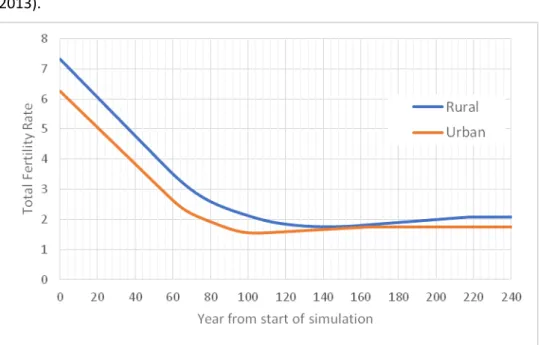
Figure 1. Fertility Pathways for Rural and Urban India modelled based on SRS* (2007, 2010‐ 2013).
Note: *Ultimate TFR are set 1.75 and 2.08 for rural and urban regions respectively
The smooth spline in Figure 1 shows that fertility declines to a level of 1.73 for rural and 1.40 for urban, and then increases (this is a phenomenon observed in many Western countries). However, it is also likely that fertility will remain at the lower level, as observed in Southeast Asia (17). Very low fertility is observed in many Northern states/UTs of India mostly among urban dwellers and could follow the Southeast Asian pattern. However, in many Southern states/UTs as well as among the most educated women, the TFR is not so low, around 1.8 (e.g., in Tamil Nadu). Further, both UN (mostly in the range of 1.6‐2.0) and WIC (1.75) assume higher levels for ultimate fertility. Based on these arguments for the Medium scenario, we assumed a TFR of 1.75 as the ultimate value at which fertility among all groups in urban regions will converge. For rural regions, we expect this ultimate level to be higher than 1.75. The gap between the ultimate fertility levels in rural and urban regions equals the gap between the minima of the two fertility pathways (0.33, see Figure 1).
The two national fertility pathways were then used to project the education‐ specific fertility in 70 sub‐regions of India. In cases where the fertility level is already below respective pathways, the gap was allowed to remain to carry forward the low fertility behavior of women in the region.
2.1.4 Our rules for fertility projections
In the following section we summarize the rules for the fertility pathway projections that we applied to our Medium scenario: 1. Fertility for women with up to completed primary education will level off at the ultimate values assumed for rural (2.08) and urban (1.75) regions. 2. Fertility for women with at least lower secondary education will follow the same path with some lag. 3. If the current value is already less than the minima, we maintained the difference. 4. Fertility for women with at least lower secondary education will stabilize at 2.08 for rural and 1.75 for urban regions. 2.1.5 Sex ratio at birth Sex ratio at birth varies spatially within India. According to the SRS 2013, the sex ratio in India is 907 girls for every 1000 boys born (952 per 1000 is considered a normal value for sex ratio at birth). The sex ratio is bit lower in urban area (901) than in the rural area (908). Between states/UTs, Northern and Northwestern states have lowest sex ratio at birth Punjab (848), Haryana (854), Uttar Pradesh (874), and less than 900 in Delhi, Rajasthan, Jammu & Kashmir, and Maharashtra. The highest value for the sex ratio was observed in Chhattisgarh (981) and closer to normal values were observed in Southern states of Kerala (966), Karnataka (948). Similar patterns of sex ratio were observed in rural and urban regions within states. For the projection, we assumed that in the next 40 years (by 2051), the sex ratio will converge to the normal value of 952 in rural and rural regions in all states/UTs.
2.2 Mortality
Sex‐specific life tables for each state/UT were downloaded from the SRS website (13), separately for rural and urban regions for 17 states/UT3. These life tables were estimated based on registered deaths during 2009‐2013. Unfortunately, the education‐specific life tables were not available at the national and the state/UT level. So far, we could not find the education‐specific mortality differential through other sources, except for infant and child mortality by mother’s educational level in the DHS. Therefore, we did not apply the education differential in mortality and left it for future updates.
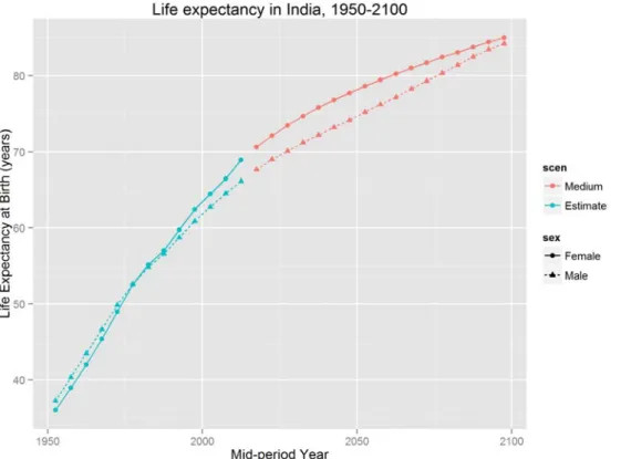
Figure 2. Life expectancy at birth among males and females in India, UN estimates and medium variant projection Source: The World Population Prospects, 2015 revision (14) In India, SRS estimates for life expectancy at birth for females and males were 69.3 years and 65.8 years respectively for the period 2009‐2013 (midyear as 2011). (13) The SRS values were slightly higher than the UN estimates for the period 2010‐2015 (midyear 2012.5), see Figure 2, with 68.9 years and 66.1 years for females and males respectively. (14)
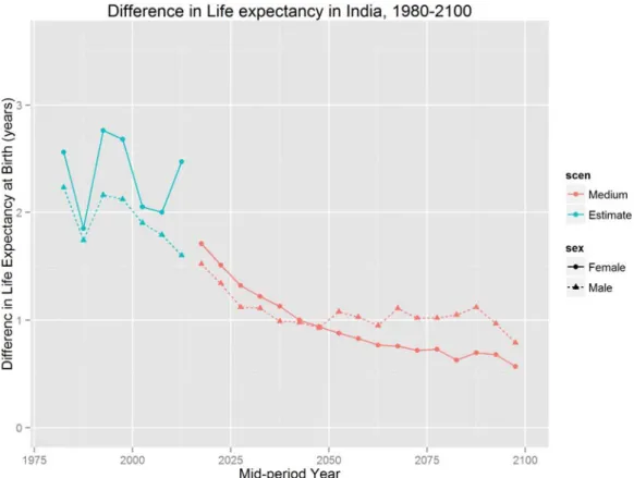
In the past, the mortality situation was worse for females. For the first time, in 1980‐85 life expectancy at birth among females (55.1 years) became higher than that for males (54.8 years), see Figure 2. The sex difference widened as the increase in life expectancy at birth for females increased faster than that for males, 2.05 vs 1.9 years (between 2000‐2005 and 2005‐2010), see Figure 3, and further widened with a gain of 2.47 vs 1.6 years for males and females respectively between the periods 2005‐2010 and 2010‐2015.
Figure 3. Gain in life expectancy at birth among males and females in India, UN estimates and medium variant projection Source: The World Population Prospects, 2015 revision (14) In UN’s medium variant, the gain in life expectancy at birth for males and females is assumed to decline in the future (see red color in Figure 3). For males, it is a continuation of the trend in the gain that stabilizes after 2040 at around one year per five years. For females, the gain for the first projection period 2015‐2010 seems to be smaller than it would have been in the case of trend extrapolation. Also, in the future the gain among females will decline further, which is a result of an implicit assumption in the UN projection that at the higher level of life expectancy, the slower the gains. .
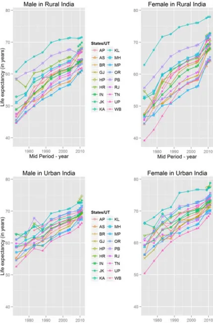
Figure 4. Life expectancy at birth in India and its 17 states, SRS estimates during 1970‐2013
Note: (AP) Andhra Pradesh, (AS) Assam, (BR) Bihar, (GJ) Gujarat, (HP) Himachal Pradesh, (HR) Haryana, (IN) India, (JK) Jammu and Kashmir, (KA) Karnataka, (KL) Kerala, (MH) Maharashtra, (MP) Madhya Pradesh, (OR) Odisha, (PB) Punjab, (RJ) Rajasthan, (TN) Tamil Nadu, (UP) Uttar Pradesh, (WB) West Bengal 2.2.1 Mortality at state level At the state level we observe that spatial diversity is very high in India. Kerala has always been a front‐runner in terms of having higher life expectancy than the rest of the country. For women in Kerala life expectancy is close to 80 years. More recently Himanchal Pradesh and Jammu & Kashmir have also shown remarkable increases in life expectancy at birth with the highest levels in urban regions. Actually, most states have already reached female urban life expectancies of above 70 years. Uttar Pradesh has the lowest urban life expectancy at birth for both men and women. Among rural areas, Madhya Pradesh, Assam, and Uttar Pradesh have the lowest levels of life expectancy at birth being the early 60s for men and mid‐60s for women. Since the 1970s
all 70 territories have seen major increases with a strong push particularly in the least developed regions since 2005, which has led to more convergence among states. The increase was particularly impressive for rural women, where in the 1970s life expectancy was in the range of 40‐50 years and now there is no state where it is below 64 years.
2.2.2 Medium assumption for mortality
In order to project life expectancy into the future, we generated an average pathway for future gain by regressing gain in life expectancy between two periods on the life expectancy of the initial period, separately for males and females. We fitted simple linear regression and extrapolated life expectancy into the future using the regression results and called it general predicted average gain. For each state/sex, we started with recently observed average rate of change and force it to converge with the general predicted average gain by 2030. Our narrative is that the convergence will carry on up until sometime in the future (we assumed it to be 2030, corresponding to the Sustainable Development Goals (SDG) target year) and then the regions will keep a similar rate of change in the future. We have set a minimum value for the general predicted average rate. When it reached a certain value, we held it constant for the rest of the future, the values are 0.75 years per five years for males and 1 year for females. This leads to a widening of the gap in life expectancy between males and females, which we think will happen in the future – following the arguments by Oeppen and Vaupel (2017) that the limit to life is not yet reached. Few rules and limitations were imposed (18): 1. The value of five‐year change in life expectancy at birth was limited to a maximum of 3 years. 2. The gain in life expectancy at birth will converge to the general predicted average gain by 2030. 3. Within each state, life expectancy in rural areas was restricted to remaining lower or equal to that in urban regions.
4. The gap between rural and urban regions was limited to the most recent observed values.
5. (Not implemented yet) The gender gap in the life expectancy is not considered yet and we will investigate further to see if it is necessary.
Once the life expectancies were ready (as shown in Figure 5), we applied the Gompertz transformation method as implemented by KC et al. (19) to produce life tables for calculated life expectancy at birth. We used the life tables for India from the UN medium variant in the World Population Prospect 2015, as standard life tables.
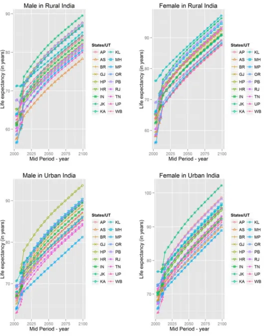
Figure 6. Life expectancy at birth in India and its 17 states, SRS estimate up till 2011 and projections thereafter – convergence to national average rate of gain by 2030
Note: (AN) Andaman and Nicobar Islands, (AP) Andhra Pradesh, (AR) Arunachal Pradesh4, (AS) Assam, (BR) Bihar, (CH) Chandigarh, (CT) Chhattisgarh, (DN) Dadra and Nagar Haveli, (DD) Daman and Diu, (DL) Delhi, (GA) Goa, (GJ) Gujarat, (HR) Haryana, (HP) Himachal Pradesh, (HR) Haryana, (IN) India, (JK) Jammu and Kashmir, (JH) Jharkhand, (KA) Karnataka, (KL) Kerala, (LD) Lakshadweep, (MH) Maharashtra, (MP) Madhya Pradesh, (MH) Maharashtra, (MN) Manipur, (ML) Meghalaya, (MZ) Mizoram, (NL) Nagaland, (OR) Odisha, (PY) Puducherry, (PB) Punjab, (RJ) Rajasthan, (SK) Sikkim, (TN) Tamil Nadu, (TR) Tripura, (UT) Uttarakhand, (UP) Uttar Pradesh, (WB) West Bengal
2.3 Migration (internal)
The internal migration between rural and urban regions within and between the states/UTs, altogether 70 spatial units, is one of the main determinants of the population dynamics in India. The data for the flow estimates between rural and urban regions by state/UT was not readily available and had to be approximated from different available tables from the Census 2001 (see Figure 6) as 2011 data is not yet published. At this point we also had to make the simplifying assumption of no international migration since reliable information is not available even at the national level. Also international estimation efforts suggest that migration levels are low with a 5‐yearly net loss of about 2 Million (20). Figure 6. Internal Migration in India by states and residence from the Census 2001
Pradesh, (MH) Maharashtra, (MN) Manipur, (ML) Meghalaya, (MZ) Mizoram, (NL) Nagaland, (OR) Odisha, (PY) Puducherry, (PB) Punjab, (RJ) Rajasthan, (SK) Sikkim, (TN) Tamil Nadu, (TR) Tripura, (UT) Uttarakhand, (UP) Uttar Pradesh, (WB) West Bengal
Following are the steps and list of data used:
i. In the first step, we extracted the data from the 2001Census5 for the total number of migrants over the last five years by sex according to current place of residence (by states/UTs and by rural/urban, destination), and by last place of residence (origin), which gives us the volume of migration flows by sex. As a next step, we estimated the age distribution of migrants at the origin and the destination.
ii. The five‐year age and sex distributions of migrants, who have been living in the current region (destination) less than 10 years (10‐yearly duration), is available by origin state/UTs and by rural/urban6. Age distribution of those who moved during the last five years would be ideal for our projections. Since the only available data is for those who moved during the last ten years, we used the 10‐yearly duration data to estimate the age and sex specific out‐ migration rates, by dividing the age‐sex‐origin‐destination specific number of migrants by the total pre‐migration population, adjusted for the flow by subtracting in‐migrants and adding out‐migrants from the total population, at the origin7. iii. A closer look at the five‐year age pattern of 10‐year duration migration rates, revealed some anomalies that called for splitting into two five‐year duration rates, as our projections will be done for five‐year age groups in five‐year time‐steps. The main problem comes from the fact that the five‐year age distribution of 10‐year duration numbers is a sum of those who moved during the last five‐years and last 5‐10 years with a five‐year lag in age. We used all the information that was available to fill the number of migrations by five‐year age and duration. The missing values were then filled using the iterative proportion fitting by employing the R package “mipfp” (21).
iv. In the next step, the five‐year number of migrations was divided by the total pre‐migration population (see Footnote8) to obtain the five‐year age and duration rates. It created a total of 9660 (70 origins x 69 destinations x 2 sexes) age patterns. Each age‐pattern was inspected visually to identify oddities and corrected if needed. Problems in the age‐pattern stem mostly from very small (even non‐existent) number of migration flows between two regions. We employed the rule that if the total amount of migration between two regions is less than 1000 persons, we apply appropriate rates for the overall pattern of migration. Corrections were also done for migration rates in the last age‐groups that were exceptionally high, mostly by smoothing or by forcing a ceiling.
5 Census 2001, Results Table D‐3: Migrants by place of last residence, duration of residence and reason for
migration
6 Census 2001, Results Table D‐12: Migrants by place of last residence with duration of residence as 0‐9
years and age
7 Migration rate = (the number of migrants) / (the number of population at origin = current population + those who left the region – those who came to the region)
2.3.1 Future assumptions We assumed that the age‐ and sex‐specific migration rates will remain constant between the 70 regions of India. With a single set of data, it is difficult to predict the trend. Once the data on migration from the 2011Census will be released, we will conduct further analyses and update our projections. One side‐effect of setting the flow rates constant, especially between urban and rural residence, is that the estimated number of people moving from urban to rural will increase in the future due to increases in the number of people living in urban areas and vice‐versa. This could result in reverse net‐migration rates between urban and rural areas. Therefore, after each reclassification of rural areas to urban, we adjusted the migration rates such that when the migration rates from rural to urban increases, the migration rate from urban to rural declines. 2.4 Urbanization The change in population size and structure in urban regions can occur due to: i) natural increase (births minus deaths); ii) migration (in‐ minus out‐), and; iii) reclassification of a rural region to urban and vice‐versa. The first two are the inherent parts of the projection model. However, urbanization through reclassification needs a separate analysis to understand what is happening and to determine how to make future assumptions. 2.4.1 Urbanization through reclassification The occurrence rate of such reclassification is difficult to predict in the future. A recent paper by Pradhan (2013) has estimated the number of villages that were classified as Census Town (CT) in the 2011 Census. The reclassification of villages to CT was based on three criteria, namely: population size, population density, and proportion of males working in non‐agriculture as main occupation. The paper estimates that almost 29.5% of the growth in urban population (91m) is due to the new CTs (Table 2 in Pradhan, 2013). No urban area in 2001 was found to be reclassified as a village by 2011. Overall, in India about 2553 new CT were reclassified from villages, with variation among states ranging from 0 (in Mizoram) and 1 (in Sikkim and Arunachal Pradesh4) to 526 in West Bengal. In Kerala, 93% of urban growth was due to reclassification (346 new CT), which highlights the migration situation to and from urban Kerala. On the contrary, in Tamil Nadu only 25% of the urban growth was due to the reclassification (227 new CT), possibly due to the attractiveness of big cities, among others Chennai, to the migrants from the rest of India. (22) We used the data presented by Pradhan (2013) to estimate the proportion of population reclassified to CT.
2.4.2 Future assumptions
In total, Bhagat (2011) estimated that in the period from 2001 to 2011 about 44% of the urban population gains were due to natural growth, while 56% were due to net reclassification, expansion of boundaries, merge of settlements and migration. Pradhan (2013) showed that 29.5% of urban growth was due to the reclassification of rural settlements into CTs and he
with a higher proportion of urban population, but additionaly, with a relatively higher socioeconomic status among the states of India. Figure 7. Proportion of population reclassified to Census Towns from rural population between 2001 and 2011 We excluded the seven outliers and fit a curve (general linear model – normally distributed error with log link function) log(y) = A+Bx, (where, y is transition ratio and x is proportion of rural population). We then let the proportion of rural population at the end of each projection period predict the transition ratio from villages to CT. We held the seven outliers constant in the future. The predicted proportion was then used to reclassify rural population to urban population. We assumed that the age‐sex‐education distribution of the reclassified population would be the same as that of the rural population. In reality, the distribution of reclassified populations could be some kind of weighted average between the rural and urban distribution. We will consider this in future updates.
2.5 Educational attainment
We defined six levels of educational attainment, namely: “no education”, “some primary”, “completed primary”, “completed lower secondary”, “completed upper secondary” and “completed post‐secondary”. The education distribution distinguished between more than six categories in the 2011 Census. We aggregated for six categories to match the International Standard Classification of Education definition (24) and studied the education transition between these six levels.
For a given educational attainment level, we defined the education attainment progression ratio (EAPR) as the proportion who completed the next level of educational attainment among those in the current level. For e.g., if in a cohort, 90% have completed at least primary education and 45% have completed at least lower secondary, then the EAPR for lower secondary completion is the ratio of the proportion of those who completed lower secondary education to those with at least primary education completed (i.e., 45%/90% = 0.5).
The education distribution in older cohorts provides information about cohort‐specific education transitions in the past, which is necessary to study the trend. Distribution and transitions from consecutive cohorts can be used to analyze the trends in different education categories (see Figure 8). Figure 8. Educational Attainment Progression Ratios in India for five educational levels among males and females by place of residence (rural and urban) in 2011 (Source: Census 2011, and own calculation) Figure 8 shows the EAPR in five‐year cohorts for rural (left panel) and urban (right panel) regions of India for five educational attainment categories (five colors) for males (dashed lines) and female (solid lines) reported in the 2011 Census.
We calculated the EAPR for five education categories, the first transition is entering or enrolling in a school for the first time; the next category is to primary completion, and so on until the post‐ secondary completion (at least first degree after the high school).
We analyzed each of the trends drawn from several cohorts and defined future education scenarios essentially by extrapolating the trend and, in some cases, by applying ‘expert’ opinions. For example, while all other transitions were allowed to become universal, the transition from upper secondary to tertiary was limited to 70% in urban and to 50% in rural areas. Also, for those regions with slower speed of change than the national pace (by state/UT, residence and sex), we allowed the speed (slope) to converge with the national one. 2.5.1 EAPR to some primary The EAPR, for at least ‘some primary’ represents the proportion of those who have ever been to school, we termed as EAPR1. India still faces the challenge of bringing everyone into the school system. Between states/UTs by place of residence, the range among age‐group 10‐14 by sex is between 77% to more than 98%. Surprisingly, among rural females in Punjab, Uttarakhand, Karnataka, and Gujarat less than 84% have ever been to school, but less developed states, such as Uttar Pradesh and Bihar, have almost universal enrolment (more than 95%). At the national level, there is no gender gap between urban areas and very little gender gap in terms of favoring boys remains in rural areas. However, at the state/residence level, the gender gap in terms of favoring males among 10‐14 year olds ranges from ‐4% to +9. At the national level, the gap between rural and urban regions is almost zero. However, the gap among 10‐14 year olds is much bigger between states/UTs in the range of ‐6% to 15% favoring urban dwellers. The worst gap is in states such as Chhattisgarh, Punjab, Gujarat. Notable exceptions were observed in Tamil Nadu and Uttar Pradesh, where the gap is in favor of rural residents.
For our projections, first we estimated the trend by linearly regressing the logit of EAPR on time. We used the logits of the EAPR because the transformed values were more linear and to make sure that the EAPR does not exceed a maximum value of 1. The trend line was estimated for each group defined by sex, type of residence and state/UT (140 lines for state/UT and 8 for India). For the first transition (EAPR for some primary) we used the data for those aged 15‐39 years (5 data points). Using the trend line we extrapolated the EAPR into the future for our Medium scenario for each group (by sex/residence/states). We visually inspected each of the 148 graphs and found that some slopes were negative and few were slow compared to the Indian average.
Therefore, in the second step, we decided to correct for the negative or slow growth by applying a convergence rule to those groups with speed (slope) less than the national slope (for the same sex and residence) to converge to the national value by 2051. Again, we visually inspected all the lines and found that in a few groups the predicted value for the next cohort in 2016, who were aged 10‐14 in 2011, was less than the empirical EAPR of the same age group in 2011. Actually, by age 10 the first transition to some primary would have taken place. However, for some population groups the transition could occur during the age‐group 10‐14 as well. To correct for the early transition, as a third step, we first repeated the steps above for the age‐ group 10‐34 and corrected the predicted values for the ‘early transition’ groups by replacing them with the new predicted values.
2.5.2 EAPR to primary
In Figure 8, the EAPR for completed primary (triangle shape in the figure) among those who went to school was the highest among all other EAPRs. This shows that once a child gets into the school, the probability that the child completes education is very high. The transition values are slightly higher in urban areas compared to rural areas and no gender gap can be observed. Between groups by states and residence (70 groups), the gender gap (females‐males) among 15‐ 19 year olds range from ‐7% (in rural Goa) to 9% (in rural Rajasthan, followed by 4% in rural Karnataka). The gap between rural and urban place of residence within states/UTs is much larger with a range from ‐4% (among males in Uttar Pradesh) to 18% (among males in Chhattisgarh). We applied the same method used for EAPR to incomplete primary, to project the EAPR of completed primary by utilizing data from the age‐group 15‐49. We also applied the same rule of convergence to those with slower slopes than the national one to converge by 2051.
2.5.3 EAPR to lower secondary
The EAPR from completed primary to lower secondary in terms of the gender gap has similar patterns as the EAPR for primary (i.e., the gap has closed). In terms of difference in the EAPR between rural and urban types of residence, the gap among 20‐24 year olds is larger among females (13%) than males (8%).
For the purpose of projections, we applied the same methods by using data from age groups 20‐ 49 (6 data points), and applied similar rules of convergence.
2.5.4 EAPR to upper secondary
For the EAPR of upper secondary in urban areas the gender gap has become negative (see Figure 8, Panel 2), with more women (83.4%) than men (81.7%) making the transition to upper secondary, among those with completed lower secondary. In rural areas the girls are speeding up to overtake boys in the near future. In the 27 mostly urban groups (by state and residence) the gender gap has reversed. The most extreme situation is in urban Uttar Pradesh where the EAPR for upper secondary is 77.4% for women compared to 65.4% among men. The highest range of the gender gap is from ‐12% to 9% in Kerala. In India, the gap in EAPR for upper secondary between rural and urban region is still significant, 15% among females and 12% among males. Except among Uttar Pradesh males (‐6%), the gap is positive with a higher EAPR in urban areas than in rural areas of states/UTs. The range is from 1% to 29% (among females in Delhi and West Bengal). For the projections, we used data from the age group 20‐40 (4 data points, including data for older ages that show a sudden jump). We applied the same methods as applied to other EAPRs, including the convergence rule. The range in the EAPR for upper secondary among 20‐24 year olds is from 41% (in rural Delhi) to 93% (in urban Himachal Pradesh). Based on the currently
Females living in urban areas are more likely to make the transition to tertiary. The highest value in a rural area is in Maharashtra with a 44% EAPR for tertiary.
Between the groups (by states/UTs and residence), the range in the gender gap among 25‐29 year olds is quite large, from ‐19% (in urban Manipur, followed by mostly urban regions) to 11% (in rural Himachal Pradesh, followed by 10% in urban Uttarakhand, and other mostly rural regions). The data shows a clear pattern, women residing in urban regions are more likely to complete tertiary than those living in rural regions.
The gap between urban and rural regions (urban minus rural) in the EAPR for tertiary is always positive, except among males in Uttar Pradesh (‐2%). The gap is very high among females, e.g., in Haryana the EAPR tertiary value is 61% in urban areas and less than half (30%) in rural areas. Such a situation is the reality in many states/UTs. However, the gap among males is also significant in many states/UTs, e.g., in Uttarakhand (26% in rural vs 51% in urban), Arunachal Pradesh4 (49% in rural vs 28% in urban) and so on. For the projection, we applied the same method and the convergence rule by using data for the age‐group 25‐49. 3 Multi‐State Demographic projection model (MS‐Dem) We used statistical software R in our calculation and have developed an R‐package named Multi‐ State Demography. This package is capable of modeling population projections by age and sex and any combination of three more dimensions, namely, education and two sub‐national dimension ‐ rural/urban and/or states/UTs in case of India. The package was released in July 2017 in R‐forge (https://r‐forge.r‐project.org/R/?group_id=2281) and the first update was released in Jan 2018.
All of the calculations were done using the statistical program R, with which we developed a package called MSDem (Multi‐State Demography). In order to give end‐users in the demographic community and local authorities (e.g., national statistical agencies) the opportunity to run their own projections, the package was made publicly available via the R‐ Forge platform in July 2017 (https://r‐forge.r‐project.org/R/?group_id=2281). The current version (0.0.2.7) was released on 2018‐01‐12.
Our package is capable of running population projections by age (A) and sex (G) in any combination with three additional dimensions, namely education (E) and two sub‐national dimensions – residence (rural/urban) (R) and state (S) (UT in case of India). This results in eight possible models: AG AGE, AGS, AGR AGES, AGER, AGSR AGESR
We cannot act on the assumption that our target audience is proficient in R programming, therefore we wanted to keep the model as simple as possible, but without losing too much flexibility at the same time. We realized that the crucial point is that the data comes in a standardized format, which we ensure by providing the users with the specific data files that need to be filled when they want to run a certain model. Then, only four steps (and three function calls) are needed to get the desired results:
1. Function state.space() helps the users generate empty data files for a given model 2. The users need to fill the empty files created in step 1 with the required data (migration numbers, fertility rates etc.) 3. Once all the data has been entered, the files are read and transformed to the required format in R 4. The simulation parameters (time horizon, reclassification assumptions etc.) are set and the simulation is run The projection results are accessible from within R, but are saved locally as .csv‐files, too. Users also have the possibility to request more detailed output. In this case, they get some standard tables and graphs that allow for a quick first glance at some of the main simulation results, e.g., the development of total population numbers, the number of deaths, the proportion of urban population etc. throughout the simulation horizon.
More detailed information about the entire process of running a population projection using MSDem can be found in the explanatory material that comes with our package.
4 Results
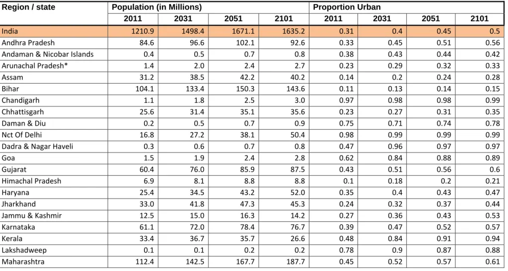
Table 1 Total population (in Millions) and proportion urban population (in %) in India and states/UTs, 2011‐2101, Medium Scenario (authors’
calculations)
Region / state Population (in Millions) Proportion Urban
2011 2031 2051 2101 2011 2031 2051 2101
India 1210.9 1498.4 1671.1 1635.2 0.31 0.4 0.45 0.5
Andhra Pradesh 84.6 96.6 102.1 92.6 0.33 0.45 0.51 0.56
Andaman & Nicobar Islands 0.4 0.5 0.7 0.8 0.38 0.43 0.44 0.42
Arunachal Pradesh* 1.4 2.0 2.4 2.7 0.23 0.29 0.32 0.33
Assam 31.2 38.5 42.2 40.2 0.14 0.2 0.24 0.28
Bihar 104.1 133.4 150.3 143.6 0.11 0.13 0.14 0.15
Chandigarh 1.1 1.8 2.5 3.0 0.97 0.98 0.98 0.99
Chhattisgarh 25.6 31.4 35.1 35.6 0.23 0.27 0.31 0.35
Daman & Diu 0.2 0.5 0.7 0.9 0.75 0.71 0.74 0.78
Nct Of Delhi 16.8 27.2 38.1 50.4 0.98 0.99 0.99 0.99
Dadra & Nagar Haveli 0.3 0.6 0.7 0.8 0.47 0.96 0.97 0.97
Goa 1.5 1.9 2.4 2.8 0.62 0.84 0.88 0.89
Gujarat 60.4 76.0 85.9 87.5 0.43 0.51 0.56 0.6
Himachal Pradesh 6.9 8.1 8.8 8.8 0.1 0.18 0.2 0.21
Haryana 25.4 34.5 43.2 52.0 0.35 0.4 0.43 0.47
Jharkhand 33.0 41.8 47.3 45.3 0.24 0.32 0.37 0.44
Jammu & Kashmir 12.5 15.0 16.3 14.2 0.27 0.36 0.43 0.53
Karnataka 61.1 72.0 78.4 76.7 0.39 0.47 0.52 0.57
Kerala 33.4 36.7 35.7 26.6 0.48 0.84 0.91 0.94
Lakshadweep 0.1 0.1 0.2 0.2 0.78 0.9 0.87 0.88
Region / state Population (in Millions) Proportion Urban 2011 2031 2051 2101 2011 2031 2051 2101 Meghalaya 3.0 3.8 4.3 4.0 0.2 0.26 0.3 0.34 Manipur 2.9 3.2 3.2 2.0 0.29 0.45 0.56 0.72 Madhya Pradesh 72.6 93.1 106.8 110.8 0.28 0.35 0.41 0.46 Mizoram 1.1 1.3 1.4 1.1 0.52 0.61 0.67 0.73 Nagaland 2.0 2.3 2.5 2.0 0.29 0.38 0.44 0.52 Odisha 42.0 48.5 51.7 48.8 0.17 0.23 0.28 0.31 Punjab 27.7 33.7 38.3 40.5 0.38 0.55 0.64 0.69 Puducherry 1.3 1.7 2.1 2.4 0.68 0.74 0.78 0.81 Rajasthan 68.6 89.9 104.1 108.9 0.25 0.3 0.34 0.37 Sikkim 0.6 0.8 0.9 0.9 0.25 0.25 0.25 0.26 Tamil Nadu 72.2 81.3 84.7 75.4 0.48 0.58 0.65 0.71 Tripura 3.7 4.2 4.3 2.8 0.26 0.46 0.57 0.68 Uttar Pradesh 199.8 256.1 284.6 262.9 0.22 0.31 0.37 0.44 Uttarakhand 10.1 13.0 15.6 17.2 0.3 0.36 0.41 0.44 West Bengal 91.3 104.4 106.2 83.3 0.32 0.47 0.56 0.66
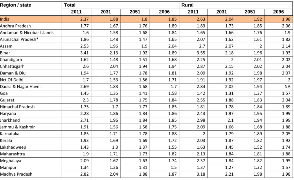
Table 2 Total Fertility Rates in India and states/UTs, 2011‐2101 Medium Scenario
Region / state Total Rural
2011 2031 2051 2096 2011 2031 2051 2096
India 2.37 1.88 1.8 1.85 2.63 2.04 1.92 1.98
Andhra Pradesh 1.77 1.67 1.76 1.89 1.83 1.73 1.85 2.06
Andaman & Nicobar Islands 1.6 1.58 1.68 1.84 1.65 1.66 1.76 1.9
Arunachal Pradesh* 1.86 1.48 1.47 1.65 2.07 1.62 1.61 1.82
Assam 2.53 1.96 1.9 2.04 2.7 2.07 2 2.14
Bihar 3.41 2.13 1.92 1.89 3.55 2.18 1.96 1.93
Chandigarh 1.62 1.48 1.51 1.68 2.25 2 2.01 2.02
Chhattisgarh 2.6 2.04 1.94 1.94 2.87 2.15 2.02 2.04
Daman & Diu 1.94 1.77 1.78 1.81 2.09 1.92 1.98 2.07
Nct Of Delhi 1.7 1.53 1.56 1.71 1.91 1.92 1.97 2
Dadra & Nagar Haveli 2.69 1.83 1.68 1.7 2.84 2.02 1.94 NA
Goa 1.45 1.35 1.41 1.58 1.42 1.31 1.37 1.57
Gujarat 2.3 1.78 1.75 1.84 2.55 1.88 1.83 2.04
Himachal Pradesh 1.75 1.7 1.77 1.85 1.81 1.78 1.84 1.89
Haryana 2.28 1.86 1.84 1.86 2.43 1.97 1.95 1.99
Jharkhand 2.71 1.96 1.84 1.85 2.98 2.1 1.94 1.99
Jammu & Kashmir 1.91 1.56 1.58 1.75 2.09 1.66 1.68 1.88
Karnataka 1.85 1.71 1.78 1.88 2 1.79 1.89 2.05 Kerala 1.93 1.69 1.69 1.72 2.03 1.87 1.82 1.92 Lakshadweep 1.43 1.3 1.37 1.55 1.63 1.45 1.52 1.74 Maharashtra 1.9 1.71 1.73 1.82 2.13 1.84 1.81 1.88 Meghalaya 2.09 1.67 1.63 1.74 2.37 1.84 1.82 1.95 Manipur 1.34 1.26 1.31 1.5 1.37 1.27 1.32 1.57 Madhya Pradesh 2.82 2.04 1.88 1.87 3.18 2.21 1.98 1.98
Region / state Total Rural 2011 2031 2051 2096 2011 2031 2051 2096 Mizoram 1.46 1.29 1.28 1.42 1.93 1.61 1.58 1.76 Nagaland 1.48 1.34 1.35 1.52 1.51 1.33 1.3 1.48 Odisha 2.13 1.83 1.86 1.93 2.28 1.94 1.98 2.01 Punjab 1.71 1.64 1.69 1.78 1.73 1.71 1.83 2.04 Puducherry 1.81 1.65 1.67 1.71 1.97 1.83 1.91 1.93 Rajasthan 2.89 2.03 1.9 1.89 3.11 2.16 2 2 Sikkim 1.53 1.43 1.44 1.66 1.55 1.45 1.46 1.7 Tamil Nadu 1.81 1.77 1.8 1.81 1.88 1.88 1.96 2 Tripura 1.38 1.22 1.22 1.41 1.47 1.32 1.35 1.6 Uttar Pradesh 3.23 2.17 1.86 1.85 3.45 2.34 1.96 1.96 Uttarakhand 2.11 1.83 1.84 1.86 2.24 1.92 1.94 1.96 West Bengal 1.73 1.5 1.5 1.67 1.92 1.68 1.75 2.03
Note: TFR is calculated using the births and population from the projection results; * A part of Arunachal Pradesh is claimed by both India and China
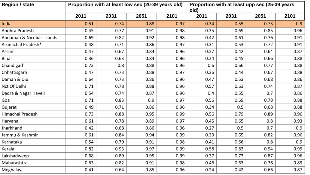
Table 3 Proportion of population aged 20 to 39 years with at least lower secondary education (in %) and proportion of population aged 20 to 39 years
with at least upper secondary education (in %) in India and states/UTs, 2011‐2101 Medium Scenario (authors’ calculations)
Region / state Proportion with at least low sec (20-39 years old) Proportion with at least upp sec (25-39 years
old)
2011 2031 2051 2101 2011 2031 2051 2101
India 0.51 0.74 0.88 0.97 0.34 0.55 0.73 0.9
Andhra Pradesh 0.45 0.77 0.91 0.98 0.35 0.69 0.85 0.96
Andaman & Nicobar Islands 0.69 0.82 0.92 0.98 0.42 0.61 0.76 0.91
Arunachal Pradesh* 0.48 0.71 0.86 0.97 0.31 0.53 0.72 0.91
Assam 0.47 0.67 0.84 0.96 0.27 0.42 0.64 0.87
Bihar 0.36 0.63 0.84 0.96 0.24 0.45 0.66 0.88
Chandigarh 0.73 0.8 0.88 0.96 0.6 0.66 0.77 0.88
Chhattisgarh 0.47 0.73 0.88 0.97 0.26 0.44 0.67 0.88
Daman & Diu 0.64 0.73 0.86 0.96 0.47 0.53 0.68 0.86
Nct Of Delhi 0.71 0.78 0.88 0.96 0.57 0.63 0.74 0.87
Dadra & Nagar Haveli 0.54 0.74 0.87 0.96 0.4 0.55 0.7 0.86
Goa 0.71 0.83 0.9 0.97 0.56 0.69 0.78 0.88
Gujarat 0.49 0.71 0.86 0.96 0.34 0.5 0.68 0.88
Himachal Pradesh 0.73 0.88 0.95 0.99 0.56 0.79 0.89 0.96
Haryana 0.61 0.78 0.89 0.97 0.45 0.65 0.8 0.93
Jharkhand 0.42 0.68 0.86 0.96 0.27 0.5 0.7 0.9
Jammu & Kashmir 0.61 0.84 0.94 0.99 0.39 0.65 0.82 0.96
Karnataka 0.54 0.79 0.91 0.98 0.41 0.66 0.8 0.9
Kerala 0.82 0.93 0.97 0.99 0.58 0.83 0.94 0.99
Lakshadweep 0.68 0.89 0.95 0.99 0.37 0.73 0.87 0.96
Maharashtra 0.63 0.82 0.91 0.98 0.46 0.63 0.76 0.89
Region / state Proportion with at least low sec (20-39 years old) Proportion with at least upp sec (25-39 years old) 2011 2031 2051 2101 2011 2031 2051 2101 Manipur 0.68 0.82 0.91 0.97 0.47 0.59 0.74 0.89 Madhya Pradesh 0.43 0.71 0.86 0.96 0.25 0.45 0.67 0.87 Mizoram 0.6 0.75 0.87 0.96 0.32 0.5 0.7 0.88 Nagaland 0.56 0.71 0.86 0.97 0.33 0.51 0.7 0.89 Odisha 0.47 0.74 0.89 0.98 0.28 0.44 0.66 0.89 Punjab 0.64 0.8 0.89 0.97 0.49 0.66 0.78 0.9 Puducherry 0.76 0.91 0.97 0.99 0.56 0.81 0.92 0.99 Rajasthan 0.42 0.68 0.86 0.96 0.24 0.47 0.69 0.9 Sikkim 0.5 0.65 0.84 0.96 0.35 0.48 0.69 0.9 Tamil Nadu 0.64 0.89 0.96 1 0.43 0.74 0.89 0.98 Tripura 0.5 0.7 0.86 0.96 0.26 0.46 0.69 0.89 Uttar Pradesh 0.48 0.73 0.86 0.96 0.29 0.53 0.71 0.9 Uttarakhand 0.66 0.83 0.91 0.98 0.45 0.63 0.75 0.89 West Bengal 0.43 0.64 0.84 0.96 0.25 0.44 0.68 0.9
References
1. Vaupel JW, Yashin AI (1985) Heterogeneity’s ruses: Some surprising effects of selection on population dynamics. Am Stat 39(3):176–185.
2. Rogers A (1995) Population forecasting: Do simple models outperform complex models? Math Popul Stud 5(3):187–202.
3. Lee RD, Carter L, Tuljapurkar S (1995) Disaggregatton in population forecasting: Do we need it? And how to do it simply. Math Popul Stud 5(3):217–234.
4. Rogers A (1995) Multiregional demography: Principles, methods and extensions (Wiley, Chichester, UK).
5. Sanderson WC (1995) Predictability, complexity, and catastrophe in a collapsible model of population, development, and environmental interactions. Math Popul Stud 5(3):259–279. 6. Long JF (1995) Complexity, accuracy, and utility of official population projections. Math
Popul Stud 5(3):203–216.
7. Lutz W, Goujon A, Doblhammer‐Reiter G (1998) Demographic dimensions in forecasting: Adding education to age and sex. Popul Dev Rev 24(Supplementary Issue: Frontiers of Population Forecasting):42–58.
8. Lutz W, KC S (2010) Dimensions of global population projections: what do we know about future population trends and structures? Philos Trans R Soc B Biol Sci 365(1554):2779– 2791.
9. Lutz W, Butz WP, KC S eds. (2014) World Population and Human Capital in the Twenty‐First
Century (Oxford University Press, Oxford, UK) Available at:
http://ukcatalogue.oup.com/product/9780198703167.do.
10. Lutz W (2017) Global Sustainable Development priorities 500 y after Luther: Sola schola et sanitate. Proc Natl Acad Sci 114(27):201702609.
11. Lutz W, Crespo Cuaresma J, Sanderson WC (2008) The demography of educational attainment and economic growth. Science 319(5866):1047–1048.
12. Census India (2011) Census of India 2011. Provisional Population Totals. Urban
Agglomerations and Cities (Office of the Registrar General & Census Commissioner,
India(RGI), Delhi, India).
13. ORGI (2014) Sample Registration System Statistical Report 2013 (Delhi, India) Available at: http://www.censusindia.gov.in/vital_statistics/SRS_Reports_2013.html.
14. United Nations (2015) World Population Prospects. The 2015 Revision. Volume 1: Comprehensive Tables (United Nations Population Division, New York).
15. WIC (2015) Wittgenstein Centre Data Explorer Version 1.2. Available at: www.wittgensteincentre.org/dataexplorer [Accessed March 18, 2015].
16. ORGI (2006) Population Projections for India and States 2001‐2026. Report of the technical
group on population projections constituted by the National Commission on Population
(Office of the Registrar General and Census Commissioner of India, Delhi, India).
17. Basten S, Sobotka T, Zeman K (2014) Future fertility in low fertility countries. World
Population and Human Capital in the 21st Century, eds Lutz W, Butz WP, KC S (Oxford
University Press, Oxford), pp 39–146.
18. Oeppen J, Vaupel JW (2017) Broken Limits to Life Expectancy. Sci Compass Policy Forum:p.3.
19. KC S, et al. (2010) Projection of populations by level of educational attainment, age, and sex for 120 countries for 2005‐2050. Demogr Res 22(Article 15):383–472.
20. Abel GJ, Sander N (2014) Quantifying global international migration flows. Science 343(6178):1520–1522.
21. Barthelemy J, Suesse T (2016) mipfp: Multidimensional Iterative Proportional Fitting and
Alternative Models. R package version 3.1. Available at: https://CRAN.R‐
project.org/package=mipfp.
22. Pradhan KC (2013) Unacknowledged Urbanisation: New Census Towns of India. Econ Polit Wkly xlviii(36):p.43‐51.
23. Bhagat RB (2011) Emerging Pattern of Urbanisation in India. Econ Polit Wkly 46(34):p.10‐ 12.
24. UNESCO (2006) International Standard Classification of Education: ISCED 1997 (Reprint) (UNESCO Institute for Statistics, Montreal, Canada).