Evaluating the provision of school performance information for school choice

THE CENTRE FOR MARKET AND PUBLIC ORGANISATION 

Centre for Market and Public Organisation  

Bristol Institute of Public Affairs  

University of Bristol  

2 Priory Road 

Bristol BS8 1TX 

http://www.bristol.ac.uk/cmpo/ 

Tel:

(0117)

33

10799

Fax:

(0117)

33

10705

E

‐

mail:

cmpo

‐

[email protected]

The Centre for Market and Public Organisation (CMPO) is a leading research  centre, combining expertise in economics, geography and law. Our objective is to  study the intersection between the public and private sectors of the economy,  and in particular to understand the right way to organise and deliver public  services. The Centre aims to develop research, contribute to the public debate and  inform policy‐making.  

CMPO, now an ESRC Research Centre was established in 1998 with two large  grants from The Leverhulme Trust. In 2004 we were awarded ESRC Research  Centre status, and CMPO now combines core funding from both the ESRC and the  Trust.  

ISSN 1473‐625X 

Evaluating the Provision of School  

Performance Information for School Choice 

Rebecca Allen and Simon Burgess

June 2010

CMPO

Working

Paper

Series

No.

10/241

Evaluating the Provision of School Performance Information 

for School Choice 

Rebecca

Allen

and

Simon

Burgess

Institute

of

Education,

University

of

London

2 

CMPO,

University

of

Bristol

June

2010

One of the key components of any school choice system is the information given to parents as the 

basis for choice.  We develop and implement a framework for determining the optimal performance 

metrics to help parents choose a school. This approach combines the three major critiques of the 

usefulness of performance tables into a natural, implementable metric. The best content for school 

performance tables is the statistic that best answers the question: “In which feasible choice school 

will a particular child achieve the highest exam score?” We implement this approach for 500,000 

students in England for a range of performance measures. Using performance tables is strongly 

better than choosing at random: a child who attends the highest ex ante performing school within 

their choice set will ex post do better than the average outcome in their choice set twice as often as 

they will do worse.     

Keywords school choice, performance tables   

JEL Classification I21, I28   

Electronic version www.bristol.ac.uk/cmpo/publications/papers/2010/wp241.pdf 

Acknowledgements 

Thanks to Department for Education for access to the NPD data, and to ESRC for funding for Burgess. 

Thanks also for comments from seminar participants at CMPO.   

Address for correspondence 

CMPO, Bristol Institute of Public Affairs 

University of Bristol 

2 Priory Road 

Bristol BS8 1TX 

2         

1.

Introduction

One of the key components of any school choice system is the information given to parents 

as the basis for choice.  For example, using both a field experiment and a natural 

experiment, Hastings and Weinstein (2008) show that the provision of information on school 

performance changed the school choice decisions of disadvantaged families towards high‐

performing schools. The publication of performance information is well established in some 

countries: performance tables showing each school’s proportion of pupils gaining five or 

more good grades have been published nationally in England since 19921; in the US, the No 

Child Left Behind (NCLB) Act of 2001 mandated publication of school‐specific performance 

measures as part of a broad drive to greater school accountability.  There is evidence that 

such information is used by parents, for example Koning and van der Wiel (2010) for the 

Netherlands and Coldron et al. (2008) and Burgess et al. (2010) for England.  Given the use 

and the impact of this information, it is clearly important to get it right: parents should be 

given performance data that is both comprehensible,2 meaning it is given to them in a metric 

that they can interpret, and functional, meaning it is a useful predictor of their own child’s 

likely exam performance.  This paper focuses on the latter. Although NCLB and other school 

choice policies rely on the assumption that it makes sense for parents to choose schools 

based on lists of schools’ test scores, Hastings and Weinstein (2008) comment “the 

relationship between school average test scores and student achievement has not been 

strongly established.” (p. 1378). We develop and implement a framework for determining 

the optimal performance metrics to help parents choose the school where their child is most 

likely to succeed academically.  We apply this framework to a range of performance 

measures to decide which metrics, if any, should be given to parents to inform school 

choice. The longevity of performance tables plus the seven years of universe pupil data now 

available in England allow us to systematically address this question for the first time. 

There is some scepticism that school performance tables are useful in choosing a school and 

several lines of critique have been presented by researchers. First, it is argued that simple 

tabulations of raw exam performance (such as graduation rates or average student test   

1

 Since then increasingly sophisticated value‐added or progress measures have supplemented the raw metrics. 

Value‐added metrics were first piloted in 1998 and introduced nationally the subsequent year; contextual value‐

added pilots were first published in 2005; and expected progress measures were first reported in 2009. 

2

scores) largely reflect differences in school composition; they do not reflect teaching quality 

and so are not informative about how one particular child might do at a school. For example, 

a school with a high average exam score might simply attract high ability pupils and there 

would therefore be no reason to expect any given student to attain a high exam score there. 

Kane and Staiger (2002) make this point in the context of performance tables as an 

accountability measure. Second, schools might be differentially effective such that even 

measures of average teaching quality or test score gains may be misleading for students at 

either end of the ability distribution. Different school practices and resources might be more 

important for gifted students or others for low ability students, and these important 

differences are lost in a single average measure.  Indeed, several studies have shown that in 

any particular year there is a difference in the estimated school effect at different parts of 

the ability distribution, though differences are not consistently found across other 

dimensions such as gender or ethnicity (Jesson and Gray, 1991; Sammons et al., 1993; 

Thomas et al., 1997; Wilson and Piebalga 2008).  Third, it is argued that the scores reported 

in performance tables are so variable over time that they cannot be reliably used to predict 

a student’s future performance. The problem of instability in performance measures was 

highlighted by Kane and Staiger (2002) in relation to the performance‐triggered sanctions in 

NCLB; they cite sampling variation and real but transient variation and small sample (school) 

sizes as the main reasons for the volatility. Leckie and Goldstein (2009) re‐emphasise this in 

the context of school league tables in England, arguing that the six year gap in time between 

school choice and exam outcome makes choice using value‐added league tables valueless. 

There is also a separate large literature that critiques the role of school performance 

information in the framework of school accountability3.   

We combine these three critiques into a single question, which we use to evaluate 

performance tables as a basis for school choice.  This provides a natural metric for judging 

the quantitative importance of all these critiques.  The question that parents want answered 

is: “In which feasible choice school will my child achieve the highest exam score?”.  We 

argue that the best content for school performance tables is the statistic that best answers   

3

 Performance tables are seen as part of a performance management system that has implicit or explicit 

incentives attached to performance outcomes (Propper and Wilson, 2003).  It is argued that certain performance 

measures can lead to dysfunctional behaviour such as manipulating admissions (see for example, Figlio and 

Getzler (2006) and Cullen and Reback (2006) for the US, West and Pennell (2000) and West (2010) for England) 

and excessive teaching to the test (for example, Wiggins and Tymms (2002) for England, Deere and Strayer 

4 

this question. Furthermore, if no performance measure can provide better guidance than 

choosing a school at random, then we would conclude that performance tables in this 

context are valueless. We address this using 6 years of universal pupil census data and 

adopting a two part empirical strategy. We identify a feasible choice set of schools for each 

student, and define a set of school choice decision rules based on different information sets 

(school performance tables). These allow us to identify the school that each pupil would 

have chosen under each decision rule. We then estimate the counterfactuals: how would 

that particular pupil have scored if they had attended that school for the following five 

years. Finally, a comparison of that outcome with a choice at random from the feasible 

choice set – that is, a choice uninformed by performance tables – tells us whether using that 

decision rule was successful for that student. We analyse this comparison across decision 

rules and across student types and areas.  

We implement this approach for half a million students in England, making a school choice 

decision in 2003 for school entry in 2004, and taking their final exams in 2009. We find that 

using (some) performance tables is strongly better than choosing at random: a child who 

attends the highest performing school within their choice set on 2003 data will ex post do 

better than the average out‐turn in their choice set twice as often as they will do worse than 

average.  We demonstrate two surprising results: first, raw outcome performance tables 

outperform sophisticated conditional outcome tables. This result derives mainly from the 

low temporal stability in the conditional outcome rankings. Second, we show that 

differential performance tables (defined below) do no better in picking the best school than 

do average performance tables. We speculate that both of these results depend in turn on 

the importance of school composition in influencing school resources and teaching quality. 

We also show that performance tables are least useful to students with small choice sets, 

and to lower ability and disadvantaged students, though no worse than choosing at random.  

The key statistical issue in the paper arises from the difficulty of estimating true school 

effects in a context where students are not randomly assigned to schools. The interpretation 

of estimated school effects as true school effectiveness is obviously an issue facing all papers 

in this field, and there is no additional problem in our approach. We discuss the possible 

biases for our results in Section 2. 

The remainder of the paper is structured as follows. Section 2 sets out our modelling 

describes the data, and section 4 presents the results and our robustness checks. Finally, 

section 5 discusses the implications of the results for the appropriate content for school 

performance tables, and for school choice. 

2.

Modelling

framework

We first set out our model of the production of pupil attainment and school actions. We 

then describe the school choice decision rules and the approach to estimating 

counterfactual outcomes for pupil attainment. 

a. The production of pupil attainment 

We adopt a fairly standard education production function, although we allow for a more 

flexible form with fewer specification assumptions (Todd and Wolpin, 2003).  For example, 

we allow for differential effectiveness, allowing the effect of each individual characteristic 

on the outcome to vary school by school.  The expected exam performance for pupil i in 

school s, Eyis, is given by: 

(

)

(

)

f

X

X

q

l

r

e

y

=

,

,

μ

,

,

,

Ε

where Xi denotes the pupil’s own characteristics that determine achievement that we 

observe in our dataset such as prior attainment, poverty status, gender and so on. Clearly, 

there are other factors influencing attainment that are not observable in standard 

administrative datasets, such as parental education, and the child’s motivation.   denotes 

the characteristics of i’s peers, the ‘pure’ peer effect, excluding the component mediated by 

school practices which we explicitly consider below. The school effect is μs, which is not 

restricted to a simple linear additive effect on top of pupil characteristics. It is useful to 

consider explicitly where this school effect comes from, and we assume it derives from a set 

of general school practices, Zs, as follows: the quality of teaching and non‐teaching staff (qs); 

the quality of leadership practices (ls) such as leadership style, policies towards behaviour, 

the strength of governance, and the monitoring of teachers; the amount and quality of 

b. The production of school resources 

One of the key insights of an economic analysis of schools is that the quality of school 

resources and practices derives from the choices of agents – headteachers, governors, 

teachers and local government. Governors appoint headteachers and take a more or less 

proactive role in school governance; heads accept or reject job offers in particular schools, 

they appoint teachers, and provide more or less inspirational and effective leadership; 

teachers also accept or reject job offers in particular schools, and help to generate effective 

teaching resources in a school. These different decisions will depend on the objectives of the 

actors and their constraints. A complete model of the outcome of this is beyond the scope of 

this paper, but the key point is that the decisions will almost certainly react to the 

environment that the actors are in. This matters because it makes it clear that the degree of 

persistence we observe in the data on school quality is behavioural, not an exogenous 

statistical process. It will in general depend on the situation a school is in, the degree of 

competition and so on. We will return to this analysis in the light of our results below. 

We assume a simple reduced form representation of those reactions. For example, although 

teachers clearly have heterogeneous preferences for school types, we assume that long‐run 

teacher quality depends on the school’s typical or expected composition,  ,4 recent past 

school exam performance, denoted  , leadership, resources and ethos, and the area the 

school is in: 

Ε

q

=

g

(

Ε

X

,

y

,

l

,

r

,

e

,

area

)

We include the area as it captures the effect of the teacher labour market, financial 

resourcing and the political control of the LA. These factors are clear influences on the 

likelihood of teachers of different quality being offered and accepting a job at a particular 

school. Similarly, we assume that the other school practices are determined in the same 

way: 

4 

It is hard to observe whether deprived schools in England actually do have lower quality teachers because 

quality is hard to estimate directly.  However, several research findings suggest they have higher teacher 

turnover and difficulties in recruitment and retention more generally (Smithers and Robinson, 2005; Dolton and 

Newsom, 2003). 

Ε

Z

=

g

(

Ε

X

,

y

,

Z

,

area

)

Z

=

q

,

l

,

r

,

e

        (3) 

where Zs‐ denotes the other three Z variables. Noting the dependence of past exam  performance on past school composition and past school quality, the long run solution to 

this will be of the form: 

Ε

Z

=

g

'

(

Ε

X

,

X

,...,

area

)

Z

=

q

,

l

,

r

,

e

That is, schools have a long‐run tendency for the quality of school practices to be strongly 

influenced by the peer and social context of the school.  Any deviations from this are likely 

to be transitory.  

Of course, the reverse dynamic is also taking place, and the school’s quality and resources 

will probably attract particular sorts of students. We return to this point below when we 

discuss selection bias into schools.  

c. School choice decision rules 

We assume that each student i faces a set ci of schools that can be chosen from. We set out 

the empirical implementation of this below. In each potential school σ  at the school choice 

date t, the distribution of exam outcomes has density function φ(y)σt. Each school choice 

decision rule is a decision to choose the highest‐performing school based on a particular 

statistic of this distribution, denoted h(φ(y)σt). The aim of this paper is to compare the 

implications of different decision rules, that is, the use of different performance statistics. 

Below we consider three main types of performance information: the fraction of students 

passing at least 5 exams (a threshold variable, a raw outcome measure); the average exam 

score of the students in the school (a continuous variable, a raw outcome measure); and a 

regression‐based conditional (or contextual) value‐added measure (a continuous, 

conditional measure). The first and third of these are the main published measures in 

England. We also consider: the average exam score differentiated for groups of students 

based on prior ability to introduce a very simple element of conditionality5; a 

       5

  This is a proposal we discuss in more depth elsewhere (Allen and Burgess, 2010); we believe it has a number of 

straightforward measure of school ability composition; and performance in maths only, and 

English only.  

Separately for each decision rule h and for each student i we identify the highest‐performing 

school in the choice set based on information available at the time of decision: 

( )

(

)

{

}

φ

σ

σ

d. Estimating school outcomes 

We need to predict the exam score outcome for each school in the choice set of each 

student. These are counter‐factuals: all bar one of these will therefore be estimated values 

for schools that that student did not actually attend (and we actually use an estimate of 

attainment for the student’s own school).  We use (1) as our starting point and to implement 

it most flexibly we estimate separate regressions for each school, and include all the 

interactions of individual characteristics we observe (see below). This allows school practices 

and resources to affect the impact of, say, prior ability on the final exam test score. The peer 

effect and the common impact of school resources are estimated in the constant term in 

each school regression.   

Having estimated the 3143 school‐by‐school regressions (not reported but summarised in 

Appendix Table 2) we use them to predict exam outcomes. We restrict the schools that we 

predict for as follows: we produce an estimated outcome only for schools in each student’s 

choice set; and we only produce estimated outcomes for schools with a minimum number of 

students similar to the focus student (detailed below). These criteria mean that we are not 

predicting too far out of sample – only for schools local to the focus student, and which 

already have students similar to the focus student. We interpret this quite conservatively to 

avoid producing estimated outcomes for contexts (schools) totally alien to the focus 

student, and which would therefore be very biased. 

There are two main issues with our estimation procedure and we consider first a 

comparison of our approach with a matching approach. Our school‐by‐school regression 

approach with (almost) all interactions of the student variables in fact gets close to 

mimicking a matching approach in allowing for very heterogeneous effects. It is important to 

recognise that matching on observables is no better at dealing with the core statistical issue  

(the non‐random assignment of students to schools) than regression; we return to this 

below. Exact matching on observables would find observationally‐equivalent students. The 

method would be to identify such students in other schools in the choice set and take the 

mean outcome for that group in that school as the predicted outcome for the focus student. 

Even with as much data as we have available, using all the variables at our disposal, exact 

matching will produce a lot of empty cells and therefore a lot of null predictions. The trade‐

off would be to use fewer variables to generate more predictions but at the cost of more 

uncontrolled heterogeneity. An alternative would be to use propensity score matching to 

introduce some smoothness and to include students who were somewhat alike to the focus 

student without restricting to exact matches. In practical terms this means running a 

matching model to identify students alike to the focus student, which implies a regression 

with a dependent variable equal to 1 for just one observation (the focus student). This 

regression would be run for each of half a million students to generate the matched set for 

each focus student. It seems highly likely that this procedure would be very noisy and 

unreliable. Given these issues, we adopt the school‐by‐school regression approach. 

The second issue is the potential effects of school selection bias. Students are not randomly 

assigned to schools and there are unobserved student characteristics that influence both the 

probability of assignment and subsequent exam performance.  We cannot model the 

assignment process explicitly and so, absent any instrument for school assignment (such as 

that used by Sacedote, 2010), we will have biased estimates of school effects.  Essentially, 

we will overestimate the quality of schools with unobservably good pupils.  This means that 

we will impute higher scores to the counterfactual pupils not at that school than they would 

truly have achieved had they attended. This is a well‐known problem and it faces all 

attempts to estimate true school effects; it is not an additional problem for our approach. 

We take two practical steps to minimise the bias. First, we use as many observable student 

characteristics as possible, including measures of student progress between ages 7 and 11 in 

some specifications to capture differences in progress from age 11 to 16.  All of these are 

interacted with other individual characteristics, again allowing for a varying impact school‐

by‐school. Descriptors for very small neighbourhood are also helpful in refining the 

characterisation of the student’s famiy background.  Second, we only consider 

counterfactual pupils for plausible local schools, and do not retain predictions for schools 

10         

We can make statements about the nature of the bias if we are prepared to explicitly 

parameterise the assignment process. Suppose we assume that the assignment mechanism   s is:  

allocating student i to school

, ;

      (6) 

where ε represents unobserved student characteristics. If a() is such that ε and μ are 

uncorrelated, then we have no problem. The case for concern is that a() implies that high ε 

students get into high μ schools, leading us to overestimate the effectiveness of those 

schools. However, while this simple assignment process will lead to biased estimates of the 

school effects – and hence of predicted student outcomes – there are important cases when 

it will not change the rank ordering of schools. Hence if the biased outcome prediction for 

student i for school σ* exceeds the average in ci, we can infer that the unbiased prediction 

would too.  

W  illustrate this as 

      (7) 

e follows. Assume a simplified attainment function: 

where X is an observable student characteristic, ε  an unobservable student characteristic 

with density function θ( ), μs the true school effect and ω is testing noise. For concreteness, 

we can think of ε  as household income.  

We assume a very simple school assignment mechanism as follows. Demand for school 

places is increasing in μs. The greater the demand, the more oversubscribed is the school 

and hence the closer to the school a family needs to live to win a place under the pervasive 

proximity condition. This is more expensive given the equilibrium in the schooling and 

housing markets, and so the greater the income required. This simple model can be 

represented as:  if , where p() is a monotonically increasing function6. 

Given this selection, if we estimate (7) by OLS the estimated constant will be: 

.       (8) 

  6

 This is obviously simplified and for example excludes X from the selection rule. This means that the OLS will 

In general, with a sufficiently regular density function θ( ), k() is a monotonically increasing 

function. In this case, the ordering of estimated school effects is the same as the ordering of 

true school effects, that is    implies  . Given the simple attainment function 

given by (7), it also then follows that if the condition E E |  is true 

for the estimated the estimated school effects, it will also hold for the true school effects. 

There are obviously important cases when this straightforward result will not hold. 

Significant variation in the parameters of (6) can be a problem. The school assignment 

process in England, which (6) summarises, is complex and varied, involving parental 

preferences and local authority rules for tie‐breaking at over‐subscribed schools, plus other 

schools that administer their own admissions (see the next section, and also West et al., 

2009). The case where the parameters of (6) are the same within the local area for each 

student again presents no problem. However, there is little we can do if the parameters of 

(6), and the consequential correlation between ε and μ, vary significantly between schools 

within a local area. Secondly, if there are quantitatively important differences in the γ 

parameter in (7) between schools, then although the result on the estimated school 

constants will still hold, it is no longer true that this carries over automatically to the 

comparison of the predicted  value in the best school and the choice set mean. But we 

emphasise, however, that this is problematic for all attempts to interpret school effects, and 

therefore for all analyses of school performance data. 

e. Assessing the performance of decision rules 

We have a feasble choice set of schools ci, an estimated outcome for each school in that set 

, and a decision rule selecting one school as the highest performing according to a 

particular performance statistic,  _ℎ . The final stage of our approach is to assess the success 

of alternative decision rules in making good choices for students.  The main question we ask 

is whether  

{

}

it Ey c

y ≥Ε ∈

Ε +6,σ* +6,σ

σ

that is, whether the student’s predicted exam performance at the ex ante ‘best’ school is 

better than the student’s average ex post exam performance across all schools in their  

choice set.  The latter is the expected value of choosing in an uninformed way, choosing at 

12 

favour the mean outcome across the choice set because it is more straightforward to 

interpret the odds ratio for small choice set sizes. 

We report other metrics, including whether a ‘good’ school chosen at random from the top 

half of the child’s choice set is better than the student’s average exam performance and 

whether a child would do worse than the average outcome in their choice set if they 

selected the school with the lowest performance on the decision rule.  We report for how 

many students this is true, and for which students.  

3.

Data

on

English

secondary

schools

Compulsory education in England lasts for 11 years, covering the primary (age 5 to 11) and 

secondary stages (age 11 to 16).  Most pupils transfer from primary to secondary school at 

age 11, although there are a few areas where this transfer is slightly different due to the 

presence of middle schools.  Secondary school allocation takes place via a system of 

constrained choice whereby parents are able to express ordered preferences for three to six 

schools anywhere in England and are offered places on the basis of published admission 

criteria that must adhere to a national Admissions Code.  Choice is administered by local 

authorities about 10 months before pupils start secondary school.  So, for example, a cohort 

who begin secondary school in September 2004 and complete their education in summer 

2009 would choose schools during the autumn of 2003 and would have access to the 

summer 2003 school performance tables. 

Parents can choose a school in one of two ways: they can choose from within a local 

‘feasible’ choice set of schools that it is possible to reach and who would accept them or 

they can choose to move house next to a desirable school.  The latter phenomenon, known 

as ‘selection by mortgage’ is widely believed to be common in England, but recent research 

suggests that the extent to which the middle classes move house to gain advantages in 

school choice may be overstated (Allen et al., 2010).  Not all local schools will accept all local 

children.  Admissions policies are complex in England, but they generally work as follows.  

First priority is usually given to pupils with a sibling already at the school, pupils with 

statements of special educational needs and children in public care.  Next, the largest 

proportion of places is allocated giving priority to children living within a designated area or 

on the basis of proximity to school.  There are also significant numbers of schools who do 

secondary pupils), priority is usually given on the basis of religious affiliation or adherence; 

other state schools offer a proportion of places on the basis of ability or aptitude for a 

particular subject (including 164 entirely selective grammars schools).  Within this very 

complex system it is estimated that around half of all pupils will not attend their nearest 

school, although this may not have been their preferred choice (Allen, 2007; Burgess et al., 

2006). 

a. The National Pupil Database (NPD) 

In this analysis we draw pupil‐level data from all eight years (2002 to 2009) of the National 

Pupil Database (NPD) to measure school performance in a variety of ways, described below.  

NPD is an administrative dataset of all pupils in the state‐maintained system, providing an 

annual census of pupils taken each year in January, from 2002 onwards (with termly 

collections since 2006).  This census of personal characteristics can be linked to each pupil’s 

test score history.  We use a single cohort to analyse the potential consequences of the 

secondary school choices made by over 500,000 pupils who transferred to secondary school 

in September 2004, completing compulsory education in 2009.  These pupils are located in 

3143 secondary schools; we exclude non‐standard schools such as special schools or those 

with fewer than 30 pupils in a cohort from the analysis.  We drop a small number of pupils 

from our analysis because they appear to be in the incorrect year group for their age or they 

have a non‐standard schooling career history. 

NPD provides data on gender (female), within‐year age (month), ethnicity (asian, black, 

othereth), an indicator of whether English is spoken at home (eal) and three indicators of 

Special Educational Needs (senstat, senplus, senact, measuring learning or behavioural 

difficulties at a high, medium and low level, respectively).  It also provides us with two 

measures of the socio‐economic background of the child.  Free School Meals (fsm) eligibility 

is an indicator of family poverty that is dependent on receipt of state welfare benefits (such 

as Income Support or Unemployment Benefit).  Our FSM variable is a very good measure of 

the FSM status of the 12 per cent of our cohort who have it, but it has been shown by Hobbs 

14         

use the Income Deprivation Affecting Children Index (idaci), an indicator for the level of 

deprivation of the household’s postcode.7 

Data on individual pupil characteristics are linked to educational attainment at the ages of 7 

(Key Stage 1 – KS1), 11 (KS2) and 16 (GCSE or equivalent examinations).  The linked test 

score data that measures the academic attainment of children in KS2 tests at the end of 

primary school serves as a useful proxy for academic success to date.  We use an overall 

score (KS2) that aggregates across all tests in English, maths and science, as well as the 

individual subject scores in our regressions (KS2eng, KS2mat, KS2sci).  We also utilise the KS1 

data recorded by teachers on children at age 7 in some specifications reported in Appendix 

Table 5.  There are some concerns about the consistency of these data because a 

component of KS1 is teacher assessed, but we believe the data quality is adequate for our 

purposes. Summary statistics of our data are presented in Appendix Table 1. 

b. Defining the choice set 

Our research question analyses the extent to which school performance tables can be used 

to make good school choices from within a local choice set.  Clearly it is impossible for us to 

know which schools any particular parent is actively considering for their child because this 

will be a function of their own preferences and constraints and the admissions policies of 

the school.  Instead, we define a choice set for every pupil that will complete school in 

summer 2009 by including a school in the choice set if another (fairly similar) pupil from the 

same neighbourhood attended the school during the eight year period of 2002 to 2009 for 

which we can observe secondary school destinations. 

The pupil’s neighbourhood is defined as a lower layer super output area (SOA), a 

geographical unit that is designed to include an approximately equal population size across 

the country.8  In our data an average of 123 pupils across eight cohorts live within an SOA.  

Our first stage of defining the pupil’s choice set is to calculate an SOA destination matrix for 

all 32,481 SOAs.  In order to avoid unusual SOA‐secondary school transfers that are caused 

by pupils moving house or coding errors, we include a school in an SOA’s destination list if 

more than two pupils from the SOA made the transfer to the secondary school over an eight   

7 

For more information see http://www.communities.gov.uk/documents/communities/pdf/131206.pdf 

(accessed 17/05/10). 

8 

year period.  SOAs have between one and 23 schools in their destination list (mean 6.11; SD 

3.19). 

We base each individual pupil’s choice set on the SOA destination list for their home address 

but introduce additional restrictions.  First, we want to exclude schools where we know the 

transfer would be impossible, so boys schools are excluded from the choice set of girls and 

academically selective grammars chools are excluded from the choice set of pupils with low 

prior (KS2) attainment.  We also need to exclude schools from the choice set if very few 

‘similar’ pupils attended the school in the main 2009 cohort because we are unable to 

estimate likely pupil outcomes if there are no similar pupils in the school.  Therefore, a 

school is excluded from a pupil’s choice set if fewer than 1% of that school’s 2009 cohort are 

of the same sex, EAL, SEN, ethnicity (white British, Asian, black, other) or KS2 group 

(indicating low, middle or high ability).  The school must also exist in both 2003 and 2009 to 

make the analysis possible; we link school openings and closings for straightforward one‐to‐

one school name/governance changes to retain as many schools as possible.  The result of 

all these restrictions is that pupil choice sets are slightly smaller than SOA destination lists: 

pupils have between one and 18 schools in their choice set (mean 5.07; SD 2.35).  Further 

descriptives of these choice sets can be found in Appendix Table 2. 

c. Calculating decision rules 

We use information on the 2003 school performance that would be available to parents 

whose children start secondary school in September 2004.  These are the decision rules that 

we use to establish whether school performance data can help parents make school choices 

that maximise their own child’s likely exam performance from within a choice set of schools.  

The decision rules that we test include metrics that have been published by the government 

and new rules that we have constructed from the underlying pupil‐level data from the 

cohort who were age 16 in 2003.  Pupils typically take nationally set, high stakes, GCSE or 

equivalent examinations in 8 to 10 subjects at the age of 16 and these are measured on an 

eight‐point pass scale from grade A*, A, B, ... to F, G.  The four main decision rules (DRs) we 

report in this paper are: 

1. Proportion of pupils achieving 5 or more GCSEs at grades A*‐C, including at least a 

16         

metric has been used to measure school performance since 1992 (with the inclusion 

of English and maths restrictions from 2006 onwards). 

2. The average grade score for pupils in their best eight subjects at GCSE 

(unconditional DR).  This score converts the grade attained by each pupil in every 

subject at GCSE and sums across the pupil’s best eight subjects.  This capped GCSE is 

not currently reported as a metric in school performance tables, but is used as the 

outcome measure for ‘contextual value added’ scores (see below).  It is regarded as 

a broad measure of performance that reflects the overall educational success of the 

child is less susceptable to gaming than the threshold measure. 

3. The average capped GCSE score for pupils at three points in the national ability 

distribution (differential DR).  We report the average school performance for pupils 

between the 20th and 30th national percentile (low); the 45th and 55th national 

percentile (middle); and the 70th to 80th national percentile (high) for each school 

and allow parents to use the decision rule that relates to their own child’s ability.  

For example, parents with pupils who are in the bottom third of the KS2 distribution 

could use the low differential capped GCSE performance measure to choose a 

school.9  This new measure of school performance evaluates how the school 

performs for pupils at different parts of the ability distribution.  In doing so it 

approximately holds constant the prior attainment of children and allows for the 

possibility that schools are differentially effective. 

4. The contextual value added score for the school, similar to that published for all 

secondary schools from 2006 (conditional DR).  This is essentially a school residual 

extracted from a multi‐level regression that conditions on the pupil and peer 

characteristics available in NPD (see Ray, 2006).  We calculate our own school CVA‐

type scores because it was not published by government in 2003. 

d. Predicting attainment across a choice set 

The most controversial part of the implementation of our method is our approach to 

predicting a pupil’s likely attainment in each school across their choice set.  We have 2009 

attainment data for this cohort and we combine this contemporaneous data with the 2008   

9

 Allen and Burgess (2010) has a discussion of the extent to which parents are aware of their child’s relative 

cohort’s attainment information to estimate each school’s achievement function through 

3143 regressions (variable names defined in Section 3a above): 

gcse

=

β

+

β

KS

2

sci

+

β

KS

2

mat

+

β

KS

2

eng

+

β

KS

2

scisq

+

β

KS

2

matsq

+

β

KS

2

engsq

+

β

fsm

+

β

idaci

+

β

idacisq

+

β

female

+

β

month

+

β

eal

+

β

asian

+

β

black

+

β

otheth

+

β

senstat

+

β

senact

+

β

senplus

+

β

female

*

fsm

+

β

female

*

idaci

+

β

female

*

asian

+

β

female

*

black

+

β

female

*

otheth

+

β

fsm

*

asian

+

β

fsm

*

black

+

β

fsm

*

otheth

+

β

fsm

*

idaci

+

β

KS

2

*

female

+

β

KS

2

*

fsm

+

β

KS

2

*

idaci

+

β

female

*

senstat

+

β

female

*

senact

+

β

female

*

senplus

+

ε

We predict pupil capped GCSE achievement for all pupils who have the school in their choice 

set, provided that there is a reasonably similar pupil at that school.  For the main 

specification we place the constraint that at least 1 percent of pupils at the school must have 

the same characteristics in terms of: KS2 group (low, middle, high), SEN type, EAL status or 

ethnicity group.  These constraints are controversial to the extent that they restrict the 

choice set of a pupil to schools attended by somewhat similar pupils, but we clearly face a 

trade‐off between wanting to generate estimates across a relevant choice set and needing 

to generate estimates that are statistically valid.10   The distribution of estimates for each 

coefficient from these school regressions is reported in Appendix Table 3. 

In our main specification that we report in the results section we combine attainment data 

from the 2008 and 2009 cohorts to estimate the school achievement functions.  We do this 

to achieve more stable estimates on coefficients, particularly for small schools and schools 

with only a small number of pupils with certain characteristics (we do not allow the 

effectiveness of a school to vary by pupil type across cohorts).  Appendix Table 5 reports 

several sensitivities to our main specifications in the appendices, including the use of 

unpooled 2009 data and the inclusion of KS1 attainment variables. 

4.

Results

This section reports the extent to which decision rules derived from 2003 English school 

performance tables are capable of helping parents identify local schools where their child        

10

 We perform a 98% Winsorisation to constrain extreme estimates.  We also set to missing estimates that are 

18 

will perform well academically in 2009.  We demonstrate the performance of our threshold 

decision rule and compare its performance to alternative rules.  These rules are more 

successful for some types of children and we explore why this might be through analysis of 

single subject performance and a decomposition of the stability of measures over time. 

a. The performance of the threshold decision rule 

We present the results in Table 1 for the 515,985 students with more than one school in 

their choice set. It shows the chances that this threshold decision rule (DR) identifies a 

school that turns out to have been a good choice.  We benchmark each decision rule against 

an uninformed choice and compute the odds ratio of making a good choice against a bad 

choice. In principle we would model an uninformed choice as a choice at random.  However, 

many students face choice sets with just 2 or 3 schools in and in this case, a literal random 

choice will produce a very high percentage of ties.  This makes the statistics hard to interpret 

because it means the odds of one random choice outperforming another random choice are 

not 1.0 (we report all statistics relative to a random choice in Appendix Table 4).  For this 

reason we compare the outcome of the decision rules with the expected value of a choice at 

random, namely the mean outcome for each student over all schools in her/his choice set.  

We consider how often choosing the best school according to the threshold DR is at least as 

good as a random choice, how often choosing a good school from the tables is at least as 

good as random, and whether the school identified by the tables as the worst choice turns 

out to be worse than random. We define a good school as one chosen at random from the 

top half of the performance table on that decision rule. 

Table 1 reports the odds that the threshold DR using 2003 data will produce an outcome 

that is better than the predicted mean average performance for the pupil across their choice 

set in 2009.  Overall, using this decision rule to select the best school in the choice set 

correctly identifies a school where the child should outperform the average across their 

choice set 1.92 times more frequently than it identifies one where the child performs worse.  

Clearly this means that a substantial fraction of students would turn out to be badly advised 

by the performance tables; but the number for whom they proved useful is almost twice as 

large. Picking a school in the top half identified by the decision rule is at least as good as 

random 1.35 times more frequently than it is worse.  Similarly, avoiding the school identified 

The remainder of the table disaggregates this performance of the decision rule by the size of 

the choice set, by the degree of variation in the choice set and by the students’ prior ability.  

The performance of this decision rule is notably greater for pupils with high prior attainment 

in KS2 tests than it is for pupils with low prior attainment.  Picking the best school according 

to the decision rule turns out to be better than random with odds of 2.92 for the top third of 

KS2 students, compared to the just 1.37 for the bottom third of KS2 students.  We return to 

explore this relationship further later in the section. 

The threshold decision rule performs better when the variation between schools (on the 

2003 decision rule measure) is greater.  This intuitively makes sense because where there 

are greater differences between schools in 2003, there should be a greater chances that the 

rank ordering is maintained over time.  It is also encouraging as it means a greater success 

rate when it matters more. 

One issue is to consider how to express uncertainty in this model. Clearly, each individual 

school regression belongs in the normal statistical framework, as do predicted outcomes 

from those. But our outcome variable, the ratio of the number students that turned out to 

have made good choices on the basis of the decision rule to the number whose choices 

turned out to be bad, is based on a complex nonlinear function of the predictions of a 

number of separate regressions. Analytically computing standard errors for this ratio is 

beyond the scope of this paper. Comparing each decision rule to a random decision seems a 

natural alternative way to do this.  Bootstrapping the entire process would be an alternative, 

but involves a number of decisions on the sample draws, for example, whether students 

should be reallocated to different choice sets of schools.  As an alternative route to 

exploring the robustness of the statistics, we report the sensitivity to alternative 

specifications in the Appendix. 

b. Comparing different decision rules 

We now compare the outcome of using the threshold DR to using the unconditional, 

differential and conditional DRs.  Table 2 is in the same format as Table 1, presenting the 

results for picking the best school according to that decision rule relative to the choice set 

mean.  At the bottom of the table we report the average Spearman’s rank correlation 

coefficient for the rank of choice set schools on the 2003 decision rule the 2009 predicted 

20         

Overall our unconditional DR (this is the school’s average capped GCSE) yields the highest 

success rate with good choices 2.04 times more frequently than bad choices.  Both the 

threshold and unconditional DRs have considerably better predictive power than the 

conditional DR, which delivers good choices only 1.33 times more frequently than bad 

choices.  This conditional DR (called CVA) was introduced to English league tables to capture 

the underlying effectiveness of the school, controlling for all measured pupil and peer 

characteristics.  However, the poor performance of CVA suggests that 2003 underlying 

effectiveness is not a particularly strong predictor of a child’s likely 2009 GCSE attainment.  

We explore some reasons for this in Table 5. 

One surprising finding is that the performance of the differential DR (this is capped GCSE 

scores at three different points in the ability distribution) is no better than that of the 

unconditional DR on which it is based. Intuition suggests that the provision of more 

information should do better; that having information on different parts of the distribution 

is more useful than just the average. The idea is that a more finely targeted decision on 

which school might be best would provide better information for students: specifically, 

students of low or high ability would be directed to schools performing differentially well for 

such students.11 However, our results show that this is not true and it actually performs 

particularly poorly for high ability pupils. 

There are several reasons why this might be the case.  It may be because schools are not 

differentially effective in a stable manner over time and we explore this further in Table 5.  

Also, differential effectiveness measures will not be more informative than raw effectiveness 

if only the size, and not the ranking, of school effects varies within a choice set at different 

parts of the ability distribution.  Within our choice set, schools do indeed have greater 

variability on the differential DR at the low ability point than the high ability point.  However, 

the Spearman's rank correlation within a choice set using our unconditional DR versus our 

differential DR at the three ability points is high at an average of around 0.7 for each 

pairwise comparison.  This observation that slopes of differential effectiveness as a function 

of ability often do not cross has been reported in other papers (e.g. Thomas et al., 1997).  A 

final advantage of the unconditional DR is that it incorporates information about school 

composition, whereas scores at different points of the distribution do not.  Table 6 explores   

11

 As discussed in the data section, we assumed that students in the bottom third of the ability distribution would 

further why the informational benefit of differential DRs is outweighed by the loss of this 

compositional information. 

c. Understanding the heterogeneity in prediction outcomes  

The decision rules we have considered yield good ex post predictions for a clear majority of 

students, but not all.  In this section we use the micro data to describe which students the 

decision rules are not useful for.  Table 3 shows the characteristics of pupils for whom we 

make poor predictions using the threshold DR.  We report the average differences in 

characteristics for these pupils and also the output from a logistic regression of the full set of 

measured pupil characteristics. 

The logistic regression confirms that location factors are important, and that a smaller 

choice set and low variation of the decision rule within the choice set both make it more 

likely that the decision rule makes a poor prediction.  Our predictions are also poorer for 

lower ability pupils, for more deprived pupils, for pupils who speak English as an additional 

language and for pupils of black or Asian ethnicity.  However, the overall explanatory power 

of the model is very low with a pseudo R‐squared of just 6.7% (and only 2.5% if we exclude 

the two location variables), so there is a great deal of randomness in the types of pupils for 

whom the decision rules make poor predictions. 

The poor performance of most decision rules for the lower ability pupils is particularly 

interesting.  This group of pupils have the greatest opportunity to influence their attainment 

through school choice, according to a variety of metrics.  For example, the correlation 

between a pupil’s own KS2 score and the standard deviation in estimated 2009 outcomes in 

the choice set is ‐0.26 in this cohort.  However, while it clearly appears to matter where 

lower ability pupils go to school, it does not appear to be possible to use published decision 

rules to particularly successfully choose a school.  This may be because the larger differences 

in apparent school effectiveness are actually due to larger unobserved pupil characteristics 

that determine attainment for this low ability group.  Alternatively, schools are indeed able 

to influence attainment a great deal for this group, but do not necessarily do so in a manner 

that is consistent over time.  Related to this, school exam entry policies for this group of 

pupils are more likely to have radically changed in response to changes in the league table 

metrics over the past decade.  The data presented in Table 5 suggests that the first 

22         

An alternative explanation of the fact that we are doing a poor job of modelling the 

potential outcomes of low ability pupils in high scoring schools is as follows. It might be that 

we can only model high performance pupils in high performance schools as it is essentially 

only that sort of pupil in those schools, and few low ability pupils actually find themselves in 

such schools. This would be troublesome for our approach, but in fact is plainly not the case. 

In our data, pupils from each quartile of the ability distribution can be found, in numbers, in 

almost every school in our data.12  

d. Single subject performance 

Table 4 presents information on the single subjects of English and maths to further explore 

why decision rules often perform poorly.  The middle column of data reports the extent to 

which using a school’s 2003 average maths GCSE successfully identifies a better than 

average child’s 2009 achievement in maths.  The odds of this a very high at 3.03, far higher 

than for any of the decision rules we have used so far to predict 2009 capped GCSE 

attainment.  The figure for English GCSE is almost as high at 2.79.  This is somewhat 

surprising since we usually find that disaggregated measures are unstable compared to an 

aggregation of several subjects.  Of course we don’t know whether this is because there 

relatively high persistent quality in a school’s maths department over a six year period or 

because there are unobserved time‐invariant cohort characteristics that strongly predict 

maths attainment.  Interestingly, maths and English DRs are capable of predicting 2009 

capped GCSE attainment almost as well as the unconditional (capped GCSE) DR does.  This 

would be true if maths or English department quality is highly related to long‐run school 

quality.  However, the more likely explanation for the relatively poor success of the 

unconditional DR is that the capped GCSE measure has been subject to considerable 

changes in the criteria about how GCSE equivalent exams are able to count in the measure.  

It has also been argued that schools can manipulate a pupil’s performance through 

introduction of certain GCSE equivalent subjects (West, 2010)  Both of these reasons mean 

that capped GCSE scores have not be as stable over time as we might expect, which reduces 

the odds of successfully using any decision rules to predict a pupil’s performance on this 

outcome measure. 

  12

 With the exception of grammar schools, but these account for fewer than 4% of pupils. For more details on 

e. Decomposing the relationship between 2003 decision rule and 2009 expected outcomes 

Where a 2003 decision rule performs relatively poorly in explaining 2009 expected outcomes 

for a child, it may do so for one (or both) of two reasons.  Firstly, schools may not be 

particularly stable in their exam performance. This would manifest itself through instability 

in the correlation between the decision rule metric in 2003 ℎ _, and the same 

metric 6 years later, ℎ _, .  However, the key issue for a parent in choosing a 

school, and for our evaluation approach, is just local stability – stability within that parent’s 

choice set; stability at a national level as reported by Leckie and Goldstein (2009) is not 

relevant to that decision. Also, only instability in metrics that produce changes in ranking are 

important since, on our performance metrics, it is the rankings of local schools that 

determine how parents choose schools. 

The second reason why a decision rule might only poorly predict a pupil’s exam performance 

is because the value of the metric for even the contemporaneous cohort, ℎ _, , is 

only weakly related to our estimate of any one specific pupil’s estimated exam performance 

at that school,  _{, ,} .  If the within‐school variance in performance was low and the 

between‐variance high we would expect the predictions based on some overall school 

metric to be good; if within‐variance is large and between‐variance low then we would 

expect poor predictions.  

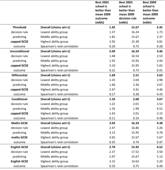
Table 5 decomposes the performance of the decision rules into these two parts.  It shows, 

for example, that the odds that the school with the highest capped GCSE score in 2003 (i.e. 

our unconditional DR) is still above the average capped GCSE in the choice set in 2009 is 

extremely high at 16.24.  The stability of the all the decision rules that measure some ‘raw’ 

performance outcome are very high.  By contrast, the stability of the differential and 

conditional DRs is relatively low within the choice set (odds ratios of 2.51 and 2.00, 

respectively).  This relatively low local stability of CVA is consistent with the low national 

stability reported by Leckie and Goldstein (2009). 

As a thought experiment, the final column reports how well using a contemporaneous 

decision rule,�