Intelligent Manufacturing
.
White Rose Research Online URL for this paper:
http://eprints.whiterose.ac.uk/153048/
Version: Accepted Version
Article:
Wang, Y, Li, K orcid.org/0000-0001-6657-0522, Gan, S et al. (1 more author) (2019)
Missing Data Imputation with OLS-based Autoencoder for Intelligent Manufacturing. IEEE
Transactions on Industry Applications, 55 (6). pp. 7219-7229. ISSN 0093-9994
https://doi.org/10.1109/tia.2019.2940585
[email protected] https://eprints.whiterose.ac.uk/ Reuse
Items deposited in White Rose Research Online are protected by copyright, with all rights reserved unless indicated otherwise. They may be downloaded and/or printed for private study, or other acts as permitted by national copyright laws. The publisher or other rights holders may allow further reproduction and re-use of the full text version. This is indicated by the licence information on the White Rose Research Online record for the item.
Takedown
If you consider content in White Rose Research Online to be in breach of UK law, please notify us by
Missing Data Imputation with OLS-based
Autoencoder for Intelligent Manufacturing
Yanxia Wang, Kang Li*, Shaojun Gan
and Che Cameron
Abstract—Motivated by a global economy that is greatly
shaped by the landscape changes in energy and man-ufacturing where more and more devices and systems are interconnected, intelligent manufacturing in which data mining is of great importance is studied. In this paper, an energy monitoring platform for small and medium-sized enterprises (SMEs) developed by the point energy team (www.pointenergy.org) is first introduced, which monitors and records the energy consumption of manufacturing processes at various levels of granularity. In processing the collected data, some incompleteness in the data due to various factors needs to be addressed first otherwise it may lead to the inaccurate portrayal of the system and poor generalisation of the resultant model trained by the data. Hence, a novel OLS (orthogonal least square)-based autoencoder is proposed to generate new samples for the imputation of missing values. This approach is to learn the representative code from the original samples by constructing an improved encoder network in which the hidden neurons are orthogonal with each other. The new samples are then generated through the decoder network. The proposed approach selects the hidden neurons one by one based on the OLS estimation until an adequate network is built. The classical techniques and other gen-erative models are compared to verify the effectiveness of the proposed algorithm. For these methods, the optimal pa-rameters are estimated based on the performance metric of cross-validation mean square error. In the experiment, the two real industrial data sets from a baking process and a polymer extrusion process are adopted and the percentage of missing values varies from 0.02 to 0.25. The experimental results confirm that the proposed method offers stable per-formance in the presence of different missing ratios, and it outperforms significantly alternative approaches while the missing ratio is greater than 0.05.
Index Terms—monitoring platform, missing data
imputa-tion, autoencoder, orthogonal least square
I. INTRODUCTION
O
VER the last decade, various issues associated to the global warming due the substantial anthropological consumption of fossil fuels have become the global concern [1]. As a con-sequence, the UK government has committed to reduce its greenhouse gas/carbon dioxide emission (GHG) by 80% by 2050 (compared to the 1990’s level) which is a huge leap Yanxia Wang, Kang Li and Shaojun Gan are with the School of Electronics and Electrical Engineering, University of Leeds, Leeds, UK (e-mail: [email protected], [email protected], [email protected]).Che Cameron is with the School of Electronics, Electrical Engineering and Computer Science, Queends University of Belfast, Belfast, UK ([email protected])
* Corresponding author.
from the current emissions levels in the past three decades [2]. As a part of this commitment to lower GHG emissions, the government has made the reduction of industrial energy consumption a priority [3]. Industrial manufacturing is one of the heavy energy consuming sectors, accounting for 16% of annual usage, and should consider the GHG reduction target as a priority [4], [5]. To gain a deep understanding of the energy consumption and to seek opportunities to improve the energy efficiency is of significant importance.
Data mining for improvement of energy efficiency has resulted in unprecedented improvements in many tasks, when given sufficient data [6], [7]. In reality, actions and decisions often need to be taken in the presence of limited datasets or in-complete datasets, due to various intentional and unintentional reasons, associated to the data generation, data collection and data transmission processes [8]. While simple extention of the measurements may not fully recover the information of the missing data. Taking the baking data set as an example, the energy consumption profile varies at different times, such as peak time and off-peak time, day and night. If the energy consumption data at the peak time is missing, then it can not be extended using the measurements taken at the off-peak time, otherwise, it may lead to quite poor generalization performance of resultant models, and the analytical results based on the data may not yield an accurate portrayal of the actual system. Therefore, techniques have been developed over the years to generate more meaningful artificial data from the original data set to improve the process modelling accuracy [9].
Multiple imputation is a widely used approach for handling the problem of incomplete data in practical applications [10], [11]. K nearest-neighbour (KNN) imputation algorithm is to find k nearest neighbours for missing data in an incomplete dataset, and then fill in the missing values with the one which has the highest probability of occurrence in neighbours if the majority rule is applied; or with the mean of neighbours if the mean rule is used. Although simple and easy to understand, to select the distance function and the number of neighbours is still a drawback for KNN [12], [13].
The random forest is a promising tree-based approach for dealing with missing data which is an extension of Breiman’s bagging idea [14], [15]. The algorithm starts with the random selection of many bootstrap samples from original data. In a normal bootstrap sample, approximately 63% of the original data occur at least one time, while the observations from the original data that do not occur are called out-of-bag. The random forest has desired characteristics of being capable of
dealing with mixed types of missing data and addressing inter-action and nonlinearity. The main limitation of this method is that a large number of trees may cost huge computation power [16]. Besides the classical algorithms, increasing attention is being paid to the ideas of generating samples from a probabil-ity distribution, which could also sort the problem of missing data. The generative adversarial networks (GAN) can represent probability distributions over observed data via an adversarial process [17]. It is a framework with two models: a generative model that captures the data distribution, and a discriminative model that estimates the probability that a sample comes from the real data rather than generator. This method has achieved great success in artificial intelligence applications, such as generating realistic images and stabilising sequence learning methods [18]–[21]. However, it is difficult to extract the real distribution features and the stochasticity in noise may not correspond to the characteristics of the real data [22]. The info generative adversarial network (infoGAN) is an extension of GAN, which could learn meaningful representations. The loss function could be interpreted as the bound of mutual information between generated data and features. While this algorithm has difficulties in learning the sample category and hence in generating class-conditional synthetic data [23].
The autoencoder is a type of neural network used to learn efficient coding in an unsupervised manner [24]. The target of this algorithm is to learn a compressed representative coding of the input, and then to decompress that code to something very close to the original input. Thus, the latent code of the autoencoder is of significant importance for generating new samples. Particle swarm optimization (PSO) is a popular algorithm for dealing with optimization problems and has been adopted to optimize the number of neurons in hidden layers (hence the number of latent variables) and the learning rate for autoencoder [25]. While for the same numbers of latent variables, the orthogonal ones could preserve the maximal amount of variance of the original input [26].
In this paper, a novel OLS (orthogonal least square)-based autoencoder approach is developed for the missing data imputation. The algorithm is an effective integration of OLS and autoencoder, which selects the hidden neurons into encoder network one by one and makes the new hidden neuron orthogonal to the existing ones. Thus, a parsimonious network with a small number of hidden neurons could be constructed as the contribution of each hidden neuron is evaluated by the OLS estimation, and the computational cost would not increase with the increase of the network complexity since only one neuron needs to be optimized by PSO in each step. The hidden neurons in the encoder are orthogonal to each other, which means the latent variables are uncorrelated, thus retaining the largest information learned from the input. To evaluate the performance of the proposed algorithm, two real industrial data sets collected by our energy monitoring platform are employed in the experiment. The classical techniques and other generative approaches are compared with the proposed method to deal with various conditions under different missing ratios.
II. PRELIMINARY WORK
A. Energy monitoring system
For intelligent manufacturing, a desire for detailed knowl-edge of operating conditions, both in terms of increased sampling rate and different granularity of use location has driven the development of the Point Energy monitoring system (www.pointenergy.org). Measurements of whole-factory as well as individual equipment are achieved using a combination of current transformers, interfaces to existing meters and customized smart meters. The system has been field-tested in different industrial sectors including a local bakery company and polymer extrusion processes. The two parts of the system can be considered as the Data Acquisition layer and the Data Analytics layer, bridged by an on-site base station, detailed in Fig. 1.
Fig. 1. The Energy monitoring system
Data acquisition mainly depends on various types of sen-sors. For instance, measurement of the electrical power is per-formed by micro-controller nodes (Multitech MDOT) that are interfaced to ABB B24 112-100 3ph power meters via Mod-bus. These meters are installed inside the factory’s electrical panels, using hardwired connections for voltage measurements with a current transformer installed at each phase to measure current. Thus, the system is capable of collecting sufficient data at different granularity to present a hologram picture of energy usage in the factory. In the bakery plant, gas and water meters produce pulse outputs which are captured via GPIO triggered interrupts. While for polymer extrusion, the temper-ature, viscosity and screw speed meters are also installed to collect corresponding signals. The gathered information is sent via the LoRaWAN radio system using the Multitech MDOT’s integrated radio, and captured by a Multitech Conduit LoRa concentrator. These LoRa packets are decoded and passed to an on-site server (standard fanless x86 hardware), which performs data concatenation and packaging before sending the readings via MQTT to off-site cloud services. The WAN connection is provided by a 3G/4G mobile signal however the router hardware is capable of taking advantage of ethernet or WiFi connections as well.
The on-site server is also responsible for node management and is capable of local data presentation, with the expecta-tion that actuator control decisions can be implemented if necessary. A dashboard is hosted on a cloud server which
presents the users with real-time (gauges and dials) and historic (searchable graphs) energy usage information. Specif-ically, electrical power categorised by different machines and production lines, gas usage rate for steam and water boilers, and the temperature of the extruder barrel, are captured and presented in the dashboard. The complete data set is stored in a secured MySQL database which can be accessed by the industrial partners and the research team through a command-line interface.
B. Problem formulation
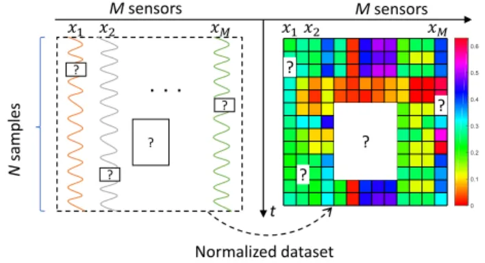
Missing values often occur due to the harsh working condi-tions or uncontrollable (unintentional or intentional) factors, such as sensors and communication failures or intentional malicious cyber attacks. The worse thing is that immediate restoration is not feasible or may cost too much. In this paper, we focus on the prediction and imputation of missing data in the collected data sets from the manufacturing sites. To give a clear illustration, Fig. 2 shows an example of dataset with missing values. In industrial dataset, since each of these dimensions in the collected data represents different signals with different scales, normalisation is required so that all the inputs are within a comparable range [27].
N sam p le s Msensors Msensors Normalized dataset t ? ? ? ? ? ? ? ?
Fig. 2. The samples of original baking data
Assume an initial data setX={xij},i= 1,2,· · ·, N, j= 1,2,· · ·, M, contains N data samples from M different sensors. Thus, the i-th data sample from j-th sensor can be donated as xij, and the data from j-th sensor in dataset
X is denoted as xj. In this paper, when xij in dataset is missing, it will be represented as ”NaN”. In addition, a matrix
Z ∈RN×M is adopted to indicate whether the value inX is missing or recorded. The elements in Z can be defined as:
zij =
0 xij =N aN
1 otherwise , (1)
wherei= 1,2,· · · , N, j= 1,2,· · · , M.
Hence, the initial data setX can be divided into incomplete subsetX′
and complete subsetX′′
. The corresponding matrix
Z′
indicates the missing values inX′
, and all the elements in
Z′′
are ones. Therefore, the problem of predicting missing data can be defined as follows: 1) Build and train the original model based on the complete dataset X′′
, and learn the knowledge representation. 2) generate and produce missing values based
encoder code decoder
input layer hidden layer hidden layer output layer
Fig. 3. The structure of autoencoder
on the updated model, learned features, incomplete datasetX′ and indicator matrixZ′
.
III. RELATEDALGORITHMS
A. Autoencoder
Autoencoder is a neural network which could be used to reconstruct high-dimensional input vectors [24]. As shown in figure 3, it first uses an adaptive, multilayer network to transform the high-dimensional data into a low-dimensional code and then a similar decoder network to generate or recover the data. This algorithm can be composed of two parts:
Encoder: This is the part of the network that compresses the input variablesXǫRN×M into a latent-space representation. It can be represented by an encoding function:
Φ =F(X), (2)
where X denotes the original input variables and Φ = [Ψ1,· · · ,ΨS] are the latent variables obtained from encoder.
Decoder: This part aims to reconstruct the input from the latent space representation. It can be represented by a decoding function:
Y =g(Φ), (3)
whereY is the output of decoder network.
Conventionally, the gradient is obtained based on the chain rule to back-propagate the error derivatives through the de-coder and ende-coder network. The cost function of this method is given by:
E=||Y −X||2= (Y −X)T(Y −X), (4) where|| · ||2 denotes the Euclidean norm.
For the back-propagate gradient descent, it is likely to converge to a local minimum when the objective function has several extreme values [28].
B. Orthogonal least squares (OLS)
For a linear-in-the-parameter model, the number of can-didate terms (or the number of hidden neurons in neural network) could be very large, which may cause over-fitting.
Thus, it is of importance to find a parsimonious model with fewer terms. Among numerical methods, matrix decomposi-tion methods have been widely adopted. In particular, OLS with QR decomposition is an well-known subset selection method for this target, having been successfully applied in many applications, such as modelling, dictionary learning and identification of nonlinear dynamic systems [29]–[31].
SupposeN data samples{xi, yi}, i= 1,2,· · · , N are used to represent model such that:
Y = Φθ+ Ξ, (5)
where Φ ∈ RS×N, Φ = [Ψ
1,· · ·,Ψj,· · · ,ΨS]T; Ψj ∈ R1×N
,Ψj = [Ψj(x1),· · ·,Ψj(xN)](j = 1,· · · , S) represents a nonlinear function of input,Ξ = [ε1,· · ·, εN]T is the noise;
θ denotes the parameter vector of the model. Thus, a cost function can be formulated as:
E= (Φθ−Y)T(Φθ−Y).
(6) If Φ is of full column rank, the least square estimation of
θ that minimizes this cost function is then given by: ˆ θ=argmin θ ||Y −Φθ||2= (Φ TΦ)−1 ΦTY, (7) and the associated minimal cost function is:
E(ˆθ) =YTY −θˆΦTY.
(8) The orthogonal transformation is introduced by OLS to produce:
Φ =W A, (9)
whereW = [w1,· · ·, wN] is an orthogonal matrix satisfying
wT
i wj= 0, ifi6=j, and A is an unit upper triangular matrix:
A= 1 α12 · · · α1S 0 1 · · · α2S .. . ... . .. ... 0 0 0 1 . (10)
Equation 5 could be rewritten as:
Y =W G+ Ξ, (11)
whereG=Aθ.
According to equation (7), the estimation ofGis computed as:
ˆ
G= (WTW)−1WTY. (12) Hence, the optimizedθˆcan be given asθˆ=A−1Gˆ, and the corresponding cost function equation (8) becomes:
E(ˆθ) =YTY − S X i=1 (YTw i)2 wT iwi . (13)
According to equation (13), the contribution of an orthogo-nal columnwito the cost function can be explicitly calculated as δEi = (YTwi)2/wTi wi without solving the least square problem.
C. Particle Swarm Optimization (PSO)
PSO was proposed by mimicking the social behaviour observed in animals, e.g., birds flocking and fish schooling [32]. With the advantages of high precision, quick convergence and easy implementation, PSO has gained increasing popular-ity among researchers as an efficient technique for solving complex optimization problems.
The algorithm begins with a swarm that the position and the velocity of each particle are generated randomly. Each potential solution is represented by a particle in the search space. Supposevi,r andxi,rbe the velocity and position of the
i-th particle in ther-th iteration;xˆi,randgrare the individual best and global best in ther-th iteration. Hence, the velocity and position ofi-th paticle at the(r+ 1)-th iteration could be updated by equation [33]:
vi,r+1←ωvi,r+c1(ˆxi,r−xi,r) +c2(gr−xi,r)
xi,r+1←xi,r+vi,r+1 , (14) whereωdenotes the inertia factor;c1andc2represent learning factors.
PSO adjusts particles at every iteration, and it will stop when the minimum error criterion or the number of iterations reaches the predefined limitation.
IV. THE PROPOSED ALGORITHM
For the proposed algorithm, OLS is adopted in the autoen-coder network. The neurons in hidden layer which are related to the features extracted from input variables are added one by one. In each step, the best neuron is selected by OLS, as OLS can select the terms that maximize the increment to the explained variance of the desired output based on the consideration of all existing candidates. Thus, an efficient OLS-based autoencoder network could be constructed.
Suppose XǫRN×M is an input matrix, where N is the number of samples andM stands for the number of dimen-sions.KM×S andb1×S are the weight matrix and bias vector between input layer and hidden layer.
In the encoder network,Sis the number of hidden neurons, namely, the number of latent variables obtained from the encoder network. If the neurons in hidden layer are orthogonal to each other, then the coordinates of the latent variables in the new S-dimensional space are uncorrelated and the maximal amount of variance of the input is preserved by only a small number of features.
Thus, the output of this algorithm Y could be written as:
Y = Ψ(X,[K, b])·θ+ Ξ, (15) whereΨ(X,[K, b])is the output of hidden layer;θrepresents the parameter matrix of weights and bias between hidden layer and output layer in decoder network.
Let Φ = Ψ(X,[K, b]), according to the orthogonal trans-formation in equation (9), the matrix can be rewritten as
W = Φ·A−1
andG=Aθ, thus
The sum of squares of the output variableY is given as: < Y, Y >= S X i=1 g2 i < wi, wi>+<Ξ,Ξ>, (17) where<> represents dot product.
The error ratio due to wi is thus defined as the proportion of the output variable variance explained by:
[err]i=
g2
i < wi, wi>
< Y, Y > . (18)
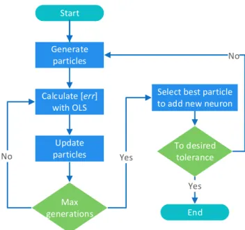
The equation (18) suggests the way of computing wi, and hence the matrix Φ, which can be used to calculate the contribution of each neuron to the output of model. Thus, the PSO algorithm could employ equation (18) as its fitness function to choose the optimal neuron for encoder in each step. As shown in figure 4, the detailed procedure is as follows.
Step 1: Add the first neuron to the hidden layer. For
i = 1,2,· · ·, D, where D denotes the number of particles;
r= 1,2,· · ·, R, whereR is the maximum of evolutionary it-eration. Every particlePi,r(thei-th particle inr-th iteration) in PSO stands for the weights and bias for the first neuron in the hidden layer, thenwi,r= Ψ
i,r·A−1, whereΨi,r = Ψ(X, Pi,r) .
Thus, the contribution of the first neuron is defined as: [err]i,r1 = (gi,r1 ) 2< wi,r 1 , w i,r 1 > < Y, Y > , (19) whereg1i,r= PQ j=1<w i,r 1 ,yj> <wi,r1 ,wi,r1 > . Assume that [err]i,r1 =max([err]
i,r
1 ,1≤i≤D,1 ≤r≤
R), which means thei-th particle from ther-th iterationPi,r is selected as the global optimal. Hence, the output of the first hidden node Ψ1 and the associated parameters θ in decoder network can be calculated.
Step 2: Add the second neuron to hidden layer. A new set of particles is generated randomly by PSO algorithm, and each particle represents the potential weights and bias. In this step, each particle to be selected is orthogonal to the first neuron. Fori= 1,2,· · ·, D andr= 1,2,· · ·, R, compute
( αi,r12 = <w1,Ψi,r> <w1,w1> wi,r2 = Ψi,r−α i,r 12·w1 , (20)
and the contribution of the second neuron is [err]i,r2 = (gi,r2 ) 2< wi,r 2 , w i,r 2 > < Y, Y > , (21) whereg2i,r= PQ j=1<w i,r 2 ,yj> <wi,r 2 ,w i,r 2 > . Assume that [err]i,r2 =max([err]
i,r
2 ,1≤i≤D,1 ≤r≤
R), thenw2=w2i,ris selected as the second column of matrix
W together with the second parameterα12=αi,r12, the second elementg2=g
i,r
2 , and[err]2= [err] i,r
2 . Therefore, the second hidden node can be confirmed.
Obviously, for the t-th neuron, we have the following equation:
Start
Generate particles
Select best particle to add new neuron
No Yes Calculate [err] with OLS Update particles Max generations To desired tolerance Yes End No
Fig. 4. The flowchart of OLS-based autoencoder
wt= Ψt− t−1 X
j=1
αjt·wj. (22) In each step, one hidden neuron is added to the neural net-work. This selection procedure continues until to the maximum number of neurons in the hidden layer or the error ratio to a desired tolerance is reached:
1− S X i=1 [err]i< ρ. (23) V. EXPERIMENTPROCEDURE A. Industrial data sets description
The details about the two industrial data sets are summa-rized in table I, both collected in real applications. There are one medium-scale baking data set with 13 attributes and one large-scale polymer data set with 20 attributes. The discussion about the experimental results will be focused on these two data sets.
1) Baking data set
In the bakery factory, a large portion of the electricity, about 30-35% is consumed in the baking process. This paper documents the initial energy consumption data set of the baking process working with three-phase 415V AC power over a randomly selected period. There are 13 sensors deployed to monitor the following features at a three-minute interval across all three phases: voltage, current, power factor, frequency, temperature, etc. Thus, the number of dimensions for each sample is 13. In the experiment, the data set is collected from baking process over a fifteen-day period with no interruption, beginning from Thursday 20th May, which consists of 7200 samples.
2) Polymer extrusion data set
Polymer extrusion is an energy intensive industrial sector, and the real-time monitoring of production process is neces-sary to meet new carbon regulations. The data set of polymer extrusion process is collected from a killion KTS-100 single-screw extruder. For the monitoring system, each measurement is constructed by the continuous collection of the 20-sensor signals, e.g. temperature, speed of screw, viscosity, and power. For the duration of two days, the length of polymer extrusion data set is 10359 in the experiment.
To simulate the reality of missing data, we select different percent of the original data and set them asN aN, namely the missing data. For the fair comparison of these methods, the missing data are randomly moved from recorded data. In the experiment, the missing ratio of the two data sets is varied by an increasing proportion—2%, 5%, 10%, 15%, 20%, and 25% respectively. Thus, we could get the data matrices D2,
D5,D10,D15,D20 andD25.
TABLE I
THE TWO DATA SETS IN THE EXPERIMENT
Data set Sensors Time Initial length
Baking data set 13 15 days 7200
Polymer extrusion data set 20 2 days 10359
B. Experimental setup 1) Compared algorithms
In this paper, to evaluate the performance of the proposed method, the classical methods are chosen based on their ef-fectiveness and popularity in solving missing data problem. In addition to autoencoder, the compared methods also include:
• K-nearest neighbour imputation (KNN): KNN impute is an algorithm that is useful for matching a point with its closest k neighbors in a multidimensional space. The assumption behind KNN is that a point value can be approximated by the points that are closest to it [34].
•Random forest (RF): The proximity between two observa-tions is the time that they end up in the same terminal node. If two observations are always in the same terminal node, their proximity will be 1. If they are never in the same terminal node, their proximity will be 0 [35].
•Generative adversarial networks (GAN): GAN is a specific generative adversarial framework of two competitive multi-layer networks, aiming to learn the data distribution from a set of samples implicitly and generate new samples from the learned distribution [36].
• Information maximizing generative adversarial networks (InfoGAN): In infoGAN, instead of using a single noise vector, the input of the Generator is decomposed into two parts: i) noise vector, which brings the variation to the new generations; ii) the latent variable, which is related to the distribution features [37].
For GAN and infoGAN, the mini-batch gradient descent (MBGD) [38] and the adaptive moment estimation (ADAM) [39] are both employed for tuning parameters.
•The denoising autoencoder (DAE) is an upgrade version of the autoencoder [40]. The idea of this algorithm is to train the
autoencoder to reconstruct the input from a corrupted version of it, thus forcing the encoder to discover more robust features and to prevent it from simply learning the identity.
In the experiment, these algorithms are implemented in Matlab version 2018a, with default parameters used, unless otherwise specified. To optimize the hyperparameters of each modelling paradigm, the cross validation is adopted with the cross-validation root mean square error (CVMSE) as the performance metric [41]. The optimal number of nearest-neighbour columns of KNN impute algorithm is selected in the range of [1, 5]. For RF algorithm, the number of trees in the forest considered ranges from 100 to 500 with the interval of 100. The number of latent code obtained in autoencoder is decided from [1, 2M/3] (rounded down), whereM is the number of attributes in the original data set. As for GANs, the architectures of Generator and Discriminator are the same, both three layers. The number of neurons in the input layer for Generator is fixed to 100. The numbers of hidden neurons for Generator and Discriminator are both selected from [100, 500]. The activation functions in the hidden and output layers are Sigmoid function and ReLU function respectively. For infoGANs, the generator and discriminator also both have a three-layer structure, and the numbers of hidden nodes are also chosen in the range of [100, 500]. The Q-net uses the Discrim-inator’s network except for the output layer—it implements own output layer. The number of nodes in output layer is set to be five, representing the number of latent variables. For mini-batch gradient descent (MBGD) and adaptive moment estimation (ADAM) training methods, the number of iterations and the initial learning rate are 100 and 0.001 respectively. For the proposed algorithm, the error ratio is set to be 0.001 and the maximum size of the latent code also can not exceed2M/3 (rounded down) with respect to the fairness.
2) Evaluation criteria
In the experiment, the datasets D2, D5, D10, D15,D20 andD25 with different percentages of missing data are used. Taking D2 for instance, the data set is divided into two data sets in line with missing values: one data set containing com-plete samples and another data set composed of incomcom-plete samples, namely with missing values. The complete data set is used for calculating and imputing the missing data in the incomplete samples according to different approaches. The expert assessment is calculated as the total mean squared error (MSE) and normalized prediction error (NPE), as the effective measures for the deviations in distances between predicted values and the observed point coordinates. The formulas for them are shown as follows:
MSE = P i,j(1−zij)(yij−yˆij)2 P ij(1−zij) (24) NPE = s P i,j(1−zij)(yij−yˆij)2 P i,j(1−zij)yi,j2 ×100% (25)
whereyij is the observed variables in the industrial dataset andyˆij is the corresponding predicted value. zij is the indi-cator matrix.
KNN 1 2 3 4 5 number of neighbors 0 0.1 0.2 0.3 0.4 0.5 0.6 CVMSE RF 100 200 300 400 500 number of trees 0 0.1 0.2 0.3 0.4 0.5 0.6 CVMSE GAN-ADAM 100 200 300 400 500 number of neurons 0 0.1 0.2 0.3 0.4 0.5 0.6 CVMSE GAN-MBGD 100 200 300 400 500 number of neurons 0 0.1 0.2 0.3 0.4 0.5 0.6 CVMSE InfoGAN-ADAM 100 200 300 400 500 number of neurons 0 0.1 0.2 0.3 0.4 0.5 0.6 CVMSE InfoGAN-MBGD 100 200 300 400 500 number of neurons 0 0.1 0.2 0.3 0.4 0.5 0.6 CVMSE Autoencoder 1 2 3 4 5 6 7 8 9
number of latent code 0 0.1 0.2 0.3 0.4 0.5 0.6 CVMSE DAE 1 2 3 4 5 6 7 8 9
number of latent code 0 0.1 0.2 0.3 0.4 0.5 0.6 CVMSE
The proposed method
1 2 3 4 5 6 7 8 9
number of latent code 0 0.1 0.2 0.3 0.4 0.5 0.6 CVMSE 2% 5% 10% 15% 20% 25%
Fig. 5. The parameter impact in baking data set
VI. EXPERIMENTAL RESULTS AND DISCUSSION
A. Parameter discussion
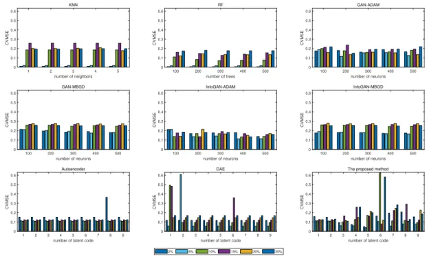
In this section, we will analyse the impact of parameter choice in the various approaches for the two data sets based on the CVMSE values. Figure 5 and figure 6 illustrate the performances of different parameters for the baking data set and polymer data set respectively.
As shown in these figures, the number of nearest neighbours has little influence to the CVMSE values for KNN. For the RF algorithm, the number of trees could affect the experimental results significantly and a moderate number of trees could perform better in most cases of varying missing ratios. For GANs and infoGANs, the number of hidden neurons reflects the structure of algorithm and the level of computational complexity in some degree. It is revealed that the performance of these algorithms would not become better along with the increase of the number of hidden neurons when the number of hidden neurons exceeds a certain threshold, which may be caused by the issue of over-fitting. Thus, the selection of pa-rameter of these algorithms should be made by considering the accuracy and the structure complexity. As for the autoencoder, the DAE technology and the proposed method, the latent codes obtained from the encoder network represents the information extracted from the original input. It is demonstrated that the size of latent code in autoencoder has only a slight impact on the performance for baking data, and this could be explained by the first few latent variables offering sufficient coverage of the features of the input data. For most percentages of missing data in polymer data set, the number of latent code in DAE could affect the experimental results largely, which indicates the selection of the latent variables is of great importance. The
superior results of the proposed method are mainly achieved when the latent code sizes are around 1/3 of the number of dimensions of input variables. In summary, the parameters in these algorithms are optimally selected based on the CVMSEs for both the baking dataset and polymer extrusion dataset are summarized in table II.
B. Results and discussion
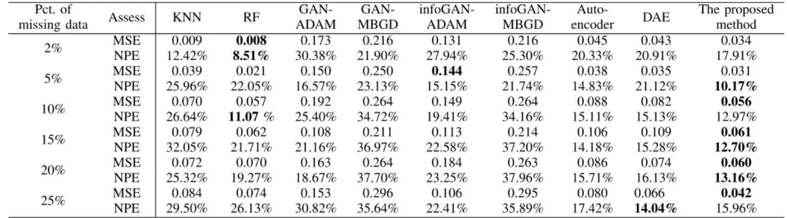
The experimental results for the baking data set are summa-rized in table III. The MSE and NPE values of the algorithms are averaged based on 100 repetitions of the experiments.
Although the MSE values of the proposed method are bigger than those of classical methods when the missing ratio is 2% and 5%, e.g. KNN and RF algorithms, the proposed method shows much better performance when the missing ratio is greater than 5%. When the missing ratios are equal to 2% and 5%, RF algorithm achieves the lowest MSE with 0.008 and 0.021, followed by KNN approach. As there are more missing values in data set, KNN and RF produce less satisfactory results, which is illustrated by the bigger MSE values. While when the missing ratio exceeds 5%, the MSEs of the proposed method are the lowest compared with other baseline models. Take missing ratio of 10% as an example, the MSE of the proposed method is lower than those of the other methods, in the magnitudes of 25.6%, 1.79%, 242.9%, 371.4%, 57.1%, and 46.4% respectively. The similar observations are found when the missing ratio varies from 15% to 25%. Furthermore, for different missing percentages, the proposed method achieves much better than autoencoder, which implies that the imple-mented OLS improves the performance of the algorithm in generating new samples.
KNN 1 2 3 4 5 number of neighbors 0 0.1 0.2 0.3 0.4 0.5 0.6 CVMSE RF 100 200 300 400 500 number of trees 0 0.1 0.2 0.3 0.4 0.5 0.6 CVMSE GAN-ADAM 100 200 300 400 500 number of neurons 0 0.1 0.2 0.3 0.4 0.5 0.6 CVMSE GAN-MBGD 100 200 300 400 500 number of neurons 0 0.1 0.2 0.3 0.4 0.5 0.6 CVMSE InfoGAN-ADAM 100 200 300 400 500 number of neurons 0 0.1 0.2 0.3 0.4 0.5 0.6 CVMSE InfoGAN-MBGD 100 200 300 400 500 number of neurons 0 0.1 0.2 0.3 0.4 0.5 0.6 CVMSE Autoencoder 1 2 3 4 5 6 7 8 9 10 11 12 13 number of latent code 0 0.1 0.2 0.3 0.4 0.5 0.6 CVMSE DAE 1 2 3 4 5 6 7 8 9 10 11 12 13 number of latent code 0 0.1 0.2 0.3 0.4 0.5 0.6 CVMSE
The proposed method
1 2 3 4 5 6 7 8 9 10 11 12 13 number of latent code 0 0.1 0.2 0.3 0.4 0.5 0.6 CVMSE 2% 5% 10% 15% 20% 25%
Fig. 6. The parameter impact in polymer data set
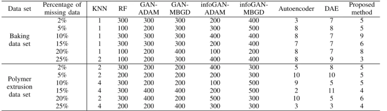
TABLE II
THE OPTIMAL PARAMETERS SELECTED FOR DIFFERENT APPROACHES
Data set Percentage of
missing data KNN RF GAN-ADAM GAN-MBGD infoGAN-ADAM infoGAN-MBGD Autoencoder DAE Proposed method Baking data set 2% 1 300 300 300 200 400 3 7 5 5% 1 100 200 300 300 500 8 8 5 10% 1 300 300 300 400 400 8 7 9 15% 1 300 300 300 200 400 7 7 6 20% 1 100 200 400 100 200 8 7 8 25% 2 100 200 300 400 400 8 9 3 Polymer extrusion data set 2% 2 300 200 200 400 300 5 8 5 5% 2 200 200 200 200 300 10 10 5 10% 4 300 200 200 100 500 9 5 5 15% 4 300 400 400 200 500 2 11 4 20% 2 300 400 200 500 300 10 5 6 25% 4 200 200 400 300 300 3 3 4
The NPE values in the experiment reveals similar results as the MSEs with the exception for missing ratio being 5% and 10%. The NPE calculated by the proposed method is the lowest when the missing ratio is 5%, which is 12% lower than that achieved by RF. The best NPE value 11.07% appearing in the condition of missing ratio being 10% is computed by RF, which means the difference between generated samples and original samples of this algorithm is the smallest. The performances of autoencoder are better than those of the DAE approach except for the conditions of missing percentage being 2% and 25%. As for NPE values, the experimental results obtained by GANs and infoGANs are very close, while the proposed method produces better results.
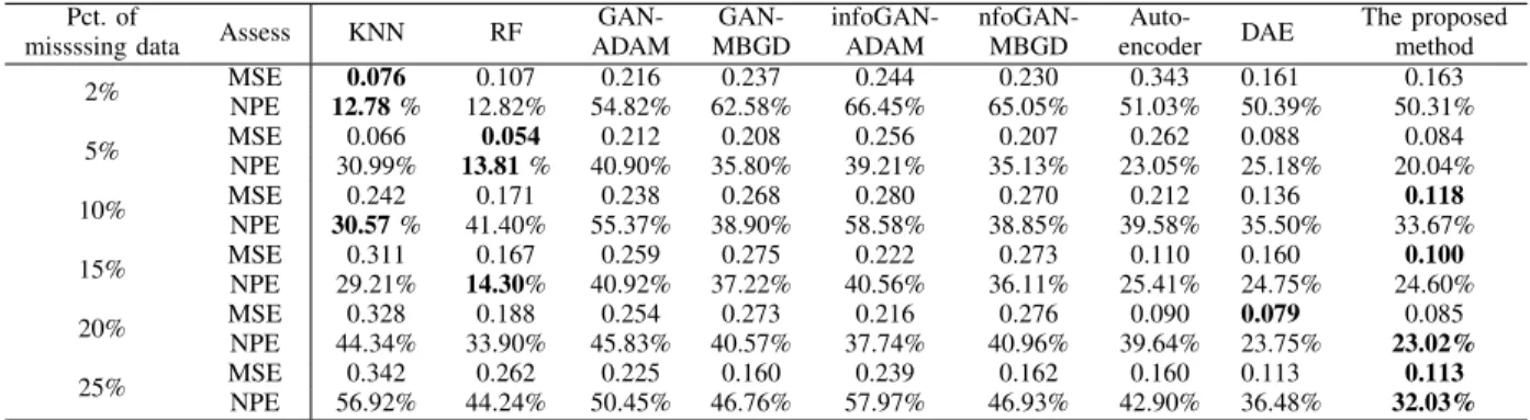
The experimental results of polymer data set are summa-rized in table IV. For fair comparisons, the expert assessment is again calculated based on the average of 100 repeated experiments. For the MSE values, the proposed approach can not perform as well as the classical methods (such as KNN and
RF) when the missing ratio is small. The KNN achieves the smallest MSE when the missing ratio is 2% and the RF obtains the best MSE when the missing ratio is 5%. The KNN and RF performs worse as the missing ratio increase, while the other generative methods offer stable performance, despite the fact that there is a little bit variation with various conditions. When the missing ratio exceeds 5%, the proposed method performs much better than the other algorithms. Although the proposed method performs slightly inferior to the DAE approach when the missing ratios are 2% and 20%, it offers better performance in the other conditions. The MSEs achieved by the proposed method are 110.4%, 211.9%, 79.7%, 10%, 5.9%, and 41.6% lower than those of autoencoder when the missing ratios vary from 2% to 25% respectively. It indicates that the integration of OLS could also improve the generative capability of the original autoencoder in dealing with the polymer data set.
For the NPE values, the proposed approach calculates the best results when the ratios are 5%, 20% and 25%. When the
TABLE III
THE EXPERIMENTAL RESULTS OF BAKING DATA SET
Pct. of
missing data Assess KNN RF
GAN-ADAM GAN-MBGD infoGAN-ADAM infoGAN-MBGD Auto-encoder DAE The proposed method 2% MSE 0.009 0.008 0.173 0.216 0.131 0.216 0.045 0.043 0.034 NPE 12.42% 8.51% 30.38% 21.90% 27.94% 25.30% 20.33% 20.91% 17.91% 5% MSE 0.039 0.021 0.150 0.250 0.144 0.257 0.038 0.035 0.031 NPE 25.96% 22.05% 16.57% 23.13% 15.15% 21.74% 14.83% 21.12% 10.17% 10% MSE 0.070 0.057 0.192 0.264 0.149 0.264 0.088 0.082 0.056 NPE 26.64% 11.07% 25.40% 34.72% 19.41% 34.16% 15.11% 15.13% 12.97% 15% MSE 0.079 0.062 0.108 0.211 0.113 0.214 0.106 0.109 0.061 NPE 32.05% 21.71% 21.16% 36.97% 22.58% 37.20% 14.18% 15.28% 12.70% 20% MSE 0.072 0.070 0.163 0.264 0.184 0.263 0.086 0.074 0.060 NPE 25.32% 19.27% 18.67% 37.70% 23.25% 37.96% 15.71% 16.13% 13.16% 25% MSE 0.084 0.074 0.153 0.296 0.106 0.295 0.080 0.066 0.042 NPE 29.50% 26.13% 30.82% 35.64% 22.41% 35.89% 17.42% 14.04% 15.96%
missing ratio is as small as 2%, the NPE value of the KNN is just 12.78%, followed by the second value obtained by the RF, while the NPE of the proposed method reaches up to 50.31%, much higher than that of classical methods. Although the NPEs of the proposed approach decrease with the increase of the missing ratio, the RF still achieves best results with the value of 13.81% and 14.3% when the missing ratio is 5% and 15% respectively. When the missing ratio is higher than 15%, the classical algorithms appear to be worse, thus the NPEs of 23.02% and 32.03% obtained by the proposed method are the smallest for the last two conditions. Although NPEs of DAE approach are smaller than those of autoencoder when missing ratios are 2% and 5%, the proposed method offers better results than the DAE approach for all missing ratios. In addition, the performances of GANs and infoGANs are stable for various missing ratios, and the effectiveness of the MBGD technique is slightly inferior to that of the ADAM approach for the most conditions with different missing ratios.
In conclusion, when the missing ratio is small, the classical imputation methods are more suitable than the generative methods. As the missing ratio increases, the performance of classical algorithms will get worse, while the proposed generative approach could can deliver stable and desirable performance. The achievements of the GANs, infoGANs and autoencoder are almost the same for different missing ratios. The DAE approach performs better than autoencoder for most missing ratios, while worse than the proposed method. In addition, the performance of the proposed approach is better than that of autoencoder for most missing ratios, which implies that the implementation of OLS could optimize the structure of the autoencoder and improve its generative capability.
VII. CONCLUSION
In this paper, the energy platform developed for small and medium-sized enterprises (SMEs) by the point energy team of the authors (www.pointenergy.org) is introduced, which can monitor and record the operating conditions of industrial machinery at different granularity levels. While analysis is hindered by the fact that data always displays some incom-pleteness due to various factors, such as measurement or transmission errors during data collection. This paper has
proposed the OLS-based autoencoder to generate new samples for missing data imputation. Advantages of this approach are as follows: i) It selects the hidden neurons one by one using the OLS estimation until an adequate network is built, which avoids redundant structure. ii)The hidden neurons of encoder are orthogonal to each other, which means the latent variables extracted from the original input are uncorrelated. iii) The computational cost does not increase with the increase of the structure complexity as only one neuron needs to be optimized at each step.
In the experiments, the classical methods and other gener-ative approaches are compared to verify the effectiveness of the proposed technique. Two real industrial data sets from a baking process and a polymer extrusion process are employed and the percentage of missing values changes between 2% to 25%. The experimental results can be concluded as follows:
• The proposed technique produces stable performance for different missing ratios.
•The classical methods, e. g. KNN and RF, are suitable for dealing with the cases of small missing ratios.
• The proposed model is competitive to other alternative approaches when the missing ratio is greater than 0.05.
•For most cases, the performance of the proposed algorithm is better than that of autoencoder, which means the implemen-tation of OLS improves its generative capability.
With these improvements, the data mining can be more rigorously conducted based on the data completeness offered by the proposed technique and more precise recommendations can thus be provided for the industrial partners.
ACKNOWLEDGMENT
This research is financially supported by the UK Engi-neering and Physical Sciences Research Council (EPSRC) under grant EP/P004636/1 ’Optimising Energy Management in Industry - ’OPTEMIN”.
REFERENCES
[1] S. Meyers, B. Schmitt, M. Chester-Jones, and B. Sturm, “Energy efficiency, carbon emissions, and measures towards their improvement in the food and beverage sector for six european countries,”Energy, vol. 104, pp. 266–283, 2016.
TABLE IV
THE EXPERIMENTAL RESULTS OF POLYMER DATA SET
Pct. of
missssing data Assess KNN RF
GAN-ADAM GAN-MBGD infoGAN-ADAM nfoGAN-MBGD Auto-encoder DAE The proposed method 2% MSENPE 12.780.076% 12.82%0.107 54.82%0.216 62.58%0.237 66.45%0.244 65.05%0.230 51.03%0.343 0.16150.39% 50.31%0.163 5% MSENPE 30.99%0.066 13.810.054% 40.90%0.212 35.80%0.208 39.21%0.256 35.13%0.207 23.05%0.262 0.08825.18% 20.04%0.084 10% MSENPE 30.570.242% 41.40%0.171 55.37%0.238 38.90%0.268 58.58%0.280 38.85%0.270 39.58%0.212 0.13635.50% 33.67%0.118 15% MSE 0.311 0.167 0.259 0.275 0.222 0.273 0.110 0.160 0.100 NPE 29.21% 14.30% 40.92% 37.22% 40.56% 36.11% 25.41% 24.75% 24.60% 20% MSE 0.328 0.188 0.254 0.273 0.216 0.276 0.090 0.079 0.085 NPE 44.34% 33.90% 45.83% 40.57% 37.74% 40.96% 39.64% 23.75% 23.02% 25% MSE 0.342 0.262 0.225 0.160 0.239 0.162 0.160 0.113 0.113 NPE 56.92% 44.24% 50.45% 46.76% 57.97% 46.93% 42.90% 36.48% 32.03%
[2] C. H. Dyer, G. P. Hammond, C. I. Jones, and R. C. McKenna, “Enabling technologies for industrial energy demand management,”Energy Policy, vol. 36, no. 12, pp. 4434–4443, 2008.
[3] P. W. Griffin, G. P. Hammond, and J. B. Norman, “Industrial energy use and carbon emissions reduction: a uk perspective,”Wiley Interdisci-plinary Reviews: Energy and Environment, vol. 5, no. 6, pp. 684–714, 2016.
[4] Y. Wang, H. Cao, X. Yan, Y. Zhou, X. Liu, and S. McLoone, “A gener-alized fuzzy linguistic model for predicting component concentrations in an optical gas sensing system,”Chemometrics and Intelligent Laboratory Systems, vol. 158, pp. 21–30, 2016.
[5] P. Agnese, M. Rizzo, and G. A. Vento, “Smes finance and bankruptcies: The role of credit guarantee schemes in the uk,” Journal of Applied Finance and Banking, vol. 8, no. 3, pp. 1–16, 2018.
[6] Z. Ma, J. Xie, H. Li, Q. Sun, Z. Si, J. Zhang, and J. Guo, “The role of data analysis in the development of intelligent energy networks,”IEEE Network, vol. 31, no. 5, pp. 88–95, 2017.
[7] Y. Wang, K. Li, S. Gan, and C. Cameron, “Analysis of energy saving potentials in intelligent manufacturing: A case study of bakery plants,”
Energy, vol. 172, pp. 477–486, 2019.
[8] R. J. Little and D. B. Rubin,Statistical analysis with missing data, vol. 333. John Wiley & Sons, 2014.
[9] A. Krizhevsky, I. Sutskever, and G. E. Hinton, “Imagenet classification with deep convolutional neural networks,” inAdvances in neural infor-mation processing systems, pp. 1097–1105, 2012.
[10] D. B. Rubin, “Multiple imputation after 18+ years,” Journal of the American statistical Association, vol. 91, no. 434, pp. 473–489, 1996. [11] P. Roystonet al., “Multiple imputation of missing values,”Stata journal,
vol. 4, no. 3, pp. 227–41, 2004.
[12] E. Acuna and C. Rodriguez, “The treatment of missing values and its effect on classifier accuracy,” inClassification, clustering, and data mining applications, pp. 639–647. Springer, 2004.
[13] J. Chen and J. Shao, “Nearest neighbor imputation for survey data,”
Journal of Official statistics, vol. 16, no. 2, p. 113, 2000.
[14] L. Breiman, “Bagging predictors,”Machine learning, vol. 24, no. 2, pp. 123–140, 1996.
[15] L. Breiman, “Random forests,”Machine learning, vol. 45, no. 1, pp. 5–32, 2001.
[16] A. Statnikov, L. Wang, and C. F. Aliferis, “A comprehensive comparison of random forests and support vector machines for microarray-based cancer classification,”BMC bioinformatics, vol. 9, no. 1, p. 319, 2008. [17] A. Antoniou, A. Storkey, and H. Edwards, “Data augmentation
genera-tive adversarial networks,”arXiv preprint arXiv:1711.04340, 2017. [18] E. L. Denton, S. Chintala, R. Fergus et al., “Deep generative image
models using a¨ı¿1
4 laplacian pyramid of adversarial networks,” in
Advances in neural information processing systems, pp. 1486–1494, 2015.
[19] A. M. Lamb, A. G. A. P. GOYAL, Y. Zhang, S. Zhang, A. C. Courville, and Y. Bengio, “Professor forcing: A new algorithm for training recur-rent networks,” inAdvances In Neural Information Processing Systems, pp. 4601–4609, 2016.
[20] M. Zhang, N. Wang, Y. Li, and X. Gao, “Neural probabilis-tic graphical model for face sketch synthesis.” arXiv preprint arXiv:10.1109/TNNLS.2018.2890017, 2019.
[21] T. Salimans, I. Goodfellow, W. Zaremba, V. Cheung, A. Radford, and X. Chen, “Improved techniques for training gans,” inAdvances in Neural Information Processing Systems, pp. 2234–2242, 2016.
[22] I. Gulrajani, F. Ahmed, M. Arjovsky, V. Dumoulin, and A. C. Courville, “Improved training of wasserstein gans,” inAdvances in Neural Infor-mation Processing Systems, pp. 5767–5777, 2017.
[23] D. K. M. T. M. D. S. J. R. J. ˚A. M. C. M. D. S. ALTUN, Y.,Machine Learning and Knowledge Discovery in Databases: part I. Springer, 2017.
[24] G. E. Hinton and R. R. Salakhutdinov, “Reducing the dimensionality of data with neural networks,”science, vol. 313, no. 5786, pp. 504–507, 2006.
[25] Jiao, Runhai and Huang, Xujian and Ma, Xuehai and Han, Liye and Tian, Wei, “A model combining stacked auto encoder and back propagation algorithm for short-term wind power forecasting,”IEEE Access, vol. 6, pp. 17 851–17 858, 2018.
[26] Mao, Jianchang and Jain, Anil K, “Artificial neural networks for feature extraction and multivariate data projection,”IEEE transactions on neural networks, vol. 6, no. 2, pp. 296–317, 1995.
[27] Y. Liu, J. Cao, B. Li, and J. Lu, “Normalization and solvability of dynamic-algebraic boolean networks,” IEEE transactions on neural networks and learning systems, vol. 29, no. 7, 2018.
[28] Y. Bengio, P. Simard, P. Frasconi et al., “Learning long-term depen-dencies with gradient descent is difficult,”IEEE transactions on neural networks, vol. 5, no. 2, pp. 157–166, 1994.
[29] S. Chen, S. A. Billings, and W. Luo, “Orthogonal least squares methods and their application to non-linear system identification,”International Journal of control, vol. 50, no. 5, pp. 1873–1896, 1989.
[30] C. Bao, J.-F. Cai, and H. Ji, “Fast sparsity-based orthogonal dictionary learning for image restoration,” inProceedings of the IEEE International Conference on Computer Vision, pp. 3384–3391, 2013.
[31] L. Zhang, K. Li, E.-W. Bai, and G. W. Irwin, “Two-stage orthogonal least squares methods for neural network construction,”IEEE transactions on neural networks and learning systems, vol. 26, no. 8, pp. 1608–1621, 2015.
[32] R. Eberhart and J. Kennedy, “A new optimizer using particle swarm theory,” inMicro Machine and Human Science, 1995. MHS’95., Pro-ceedings of the Sixth International Symposium on, pp. 39–43. IEEE, 1995.
[33] Y. Shi and R. C. Eberhart, “Fuzzy adaptive particle swarm optimization,” inProceedings of the 2001 congress on evolutionary computation (IEEE Cat. No. 01TH8546), vol. 1, pp. 101–106. IEEE, 2001.
[34] P. J. Garc´ıa-Laencina, J.-L. Sancho-G´omez, A. R. Figueiras-Vidal, and M. Verleysen, “K nearest neighbours with mutual information for simul-taneous classification and missing data imputation,” Neurocomputing, vol. 72, no. 7-9, pp. 1483–1493, 2009.
[35] C. Zhang and Y. Ma,Ensemble machine learning: methods and appli-cations. Springer, 2012.
[36] I. Goodfellow, J. Pouget-Abadie, M. Mirza, B. Xu, D. Warde-Farley, S. Ozair, A. Courville, and Y. Bengio, “Generative adversarial nets,” inAdvances in neural information processing systems, pp. 2672–2680, 2014.
[37] X. Chen, Y. Duan, R. Houthooft, J. Schulman, I. Sutskever, and P. Abbeel, “Infogan: Interpretable representation learning by information maximizing generative adversarial nets,” inAdvances in neural informa-tion processing systems, pp. 2172–2180, 2016.
[38] S. Ruder, “An overview of gradient descent optimization algorithms,”
arXiv preprint arXiv:1609.04747, 2016.
[39] D. P. Kingma and J. Ba, “Adam: A method for stochastic optimization,”
[40] Vincent, Pascal and Larochelle, Hugo and Bengio, Yoshua and Man-zagol, Pierre-Antoine, “Extracting and composing robust features with denoising autoencoders,” inProceedings of the 25th international con-ference on Machine learning, pp. 1096–1103. ACM, 2008.
[41] G. Gong, “Cross-validation, the jackknife, and the bootstrap: excess
error estimation in forward logistic regression,”Journal of the American Statistical Association, vol. 81, no. 393, pp. 108–113, 1986.