Multi Sensor Fusion Based Framework For Efficient Mobile Robot Collision Avoidance and Path Following System

(1)

MULTI SENSOR FUSION BASED FRAMEWORK FOR

EFFICIENT MOBILE ROBOT COLLISION

AVOIDANCE AND PATH FOLLOWING SYSTEM

Marwah Almasri

Under the Supervision of Prof. Khaled Elleithy

DISSERTATION

SUBMITTED IN PARTIAL FULFILMENT OF THE REQUIREMENTS

FOR THE DEGREE OF DOCTOR OF PHILOSOPHY IN COMPUTER SCIENCE

AND ENGINEERING

THE SCHOOL OF ENGINEERING

UNIVERSITY OF BRIDGEPORT

CONNECTICUT

(2)

(3)

iii

MULTI SENSOR FUSION BASED FRAMEWORK FOR

EFFICIENT MOBILE ROBOT COLLISION AVOIDANCE AND

PATH FOLLOWING SYSTEM

(4)

iv

MULTI SENSOR FUSION BASED FRAMEWORK FOR

EFFICIENT MOBILE ROBOT COLLISION AVOIDANCE AND

PATH FOLLOWING SYSTEM

ABSTRACT

The field of autonomous mobile robotics has recently gained the interests of many researchers. Due to the specific needs required by various applications of mobile robot systems (especially in navigation), designing a real-time obstacle avoidance and path following robot system has become the backbone of controlling robots in unknown environments. Therefore, an efficient collision avoidance and path following methodology is needed to develop an intelligent and effective autonomous mobile robot system. Mobile robots are equipped with various types of sensors (such as GPS, camera, infrared and ultrasonic sensors); these sensors are used to observe the surrounding environment. However, these sensors sometimes fail and have inaccurate readings. Therefore, the integration of sensor fusion will help to solve this dilemma and enhance the overall performance.

A new technique for line following and collision avoidance in the mobile robotic systems is introduced. The proposed technique relies on the use of infrared sensors and

(5)

v

involves a reasonable level of calculations, to be easily used in real-time control applications.

In addition, a fusion model based on fuzzy logic is proposed. Eight distance sensors and a range finder camera are used for the collision avoidance approach, where three ground sensors are used for the line or path following approach. The fuzzy system is composed of nine inputs (which are the eight distance sensors and the camera), two outputs (which are the left and right velocities of the mobile robot’s wheels), and twenty four fuzzy rules for the robot’s movement.

Webots Pro simulator is used for modeling the environment and robot to show the ability of the robot to follow a path, detect obstacles, and navigate around them to avoid collision. It also shows that the robot has been successfully following extremely congested curves and has avoided any obstacle that emerged on its path.

The proposed methodology which includes the collision avoidance based on fuzzy logic fusion model and line following robot, has been implemented and tested through simulation and real-time experiments. Various scenarios have been presented with static and dynamic obstacles, using one and multiple robots while avoiding obstacles in different shapes and sizes. The proposed methodology reduced the traveled distance of the mobile robot, as well as minimized the energy consumption and the distance between the robot and the obstacle detected as compared to a non-fuzzy logic approach.

(6)

vi

DEDICATION

To my mother (Efaqat Ezmirly), and to the memory of my father

(Mohammad),

(7)

vii

ACKNOWLEDGEMENTS

My thanks are wholly devoted to God who has helped me all the way to complete this work successfully.

I would like to express my special appreciation and thanks to my advisor Prof. Khaled Elleithy for his continuous support, patience, and motivation towards my Ph.D study and research. I am indebted to him for sharing his expertise and valuable guidance. Without his support and insight, this work would have never been accomplished. Prof. Khaled Elleithy, I would like to thank you very much for the dedicated time, assistance, and thoughtful comments you provided throughout the process.

I would also like to extend my appreciation to Prof. Magdy Bayoumi for his support, feedback, and insightful comments about my work. I am expressing my deepest gratitude to the committee members: Prof. Junling Hu, Prof. Xingguo Xiong, and Prof. Miad Faezipour; for their guidance, suggestions, and support.

A special thanks goes to my lovely mother, brothers (Ahmad, Bakr, and Omar), and sisters (Maha, Manal, and Rawan) for their support over the past years. Words cannot express how grateful I am for your prayers and encouragement; that is what sustained me this far. Finally, I would like to thank my best friend and sister Abrar Alajlan for the constant support and encouragement. I am sure that our friendship will last a lifetime.

(8)

viii

ACRONYMS

DoS Denial of Service

ATR Automatic Target Recognition

MAP Maximum A Posteriori

ML Maximum Likelihood

pdf Probability density function

SMC Sequential Monte Carlo

MMSE Minimum Mean Square Error

EKF Extended Kalman Filter

UKF Unscented Kalman Filter

MLE Maximum Likelihood Estimator

DSP Digital Signal Processing

DSC Distributed Source Coding

DISCUS Distributed Source Coding Using Syndromes

(9)

ix

Webots Pro Mobile robot simulator software

GUI Graphical User Interface

LFA Line Follower Approach

CCA Collision Avoidance Approach

TIME_STEP The time of one step of the simulation time

d Number of distance sensors

g Number of ground sensors

thr Collision avoidance threshold

s Mobile robot’s global speed

fs Mobile robot’s offset speed

ls Mobile robot’s left motor speed

rs Mobile robot’s right motor speed

Δ The difference between the right and left ground sensors

ANFIS Adaptive Neuro-Fuzzy Inference System

AGV Autonomous Ground Vehicle

(10)

x

OAM Obstacle Avoidance Module

LFM Line Flowing Module

LEM Line Entering Module

LLM Line Leaving Module

UTM U-Turn Module

FLS Fuzzy Logic System

LV Left velocity

RV Right velocity

FIS Fuzzy Inference System

OBSNF Obstacle not found membership function

OBSF Obstacle found membership function

Near Range finder camera near distance membership function

FAR Range finder camera far distance membership function

NEG_V Negative velocity

(11)

xi

LIST OF TABLES

Table 2.1 Code by ordering example. 19

Table 2.2 Comparison of data fusion techniques. 30

Table 4.1 Summarizes all distance sensors measurements at different simulation times.

45

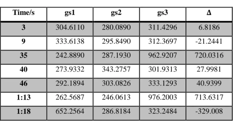
Table 4.2 Summarizes all ground sensors readings and Δ values at different simulation times.

46

Table 5.1 Fuzzy logic rules. 57

Table 5.2 Distance sensors values before and after implementing the fusion model.

65

Table 5.3 Distance measurements by camera before and after implementing the fusion model.

65

Table 5.4 Ground sensors values at different simulation times 65 Table 5.5 The position, orientation, and velocities of the robot in a

simple environment

(15)

xv

Table 5.6 The position and orientation of both robots at different simulation times.

74

Table 5.7 Summaries of the robot’s position and rotation angle at various simulation times.

77

Table 6.1 The comparison between the proposed technique and the other techniques

(16)

xvi

LIST OF FIGURES

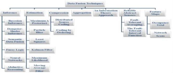
Figure 2.1 Data fusion techniques 8

Figure 2.2 The deduction and abduction example 13

Figure 2.3 Kalman filter block diagram 16

Figure 2.4 An example of DISCUS data compression 19

Figure 2.5 Two different scenarios of applying the "Fault-Tolerant Averaging" algorithm where there is one faulty sensor.

24

Figure 2.6 Two different scenarios of applying The "Fault-Tolerant Interval" (FTI) function

24

Figure 3.1 Webots Pro simulator overview 34

Figure 3.2 Schematic drawing of distance sensors in the E-puck robot. 35

Figure 3.3 Ground sensors for the E-puck robot. 35

Figure 3.4 The real E-puck robot 35

Figure 4.1 Block diagram of the proposed technique 37

Figure 4.2 Line follower and collision avoidance Algorithm. 39

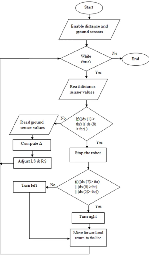
Figure 4.3 Flowchart of the proposed method. 40

Figure 4.4 Robot platform of the simulation where there are two obstacles placed on the robot path

(17)

xvii

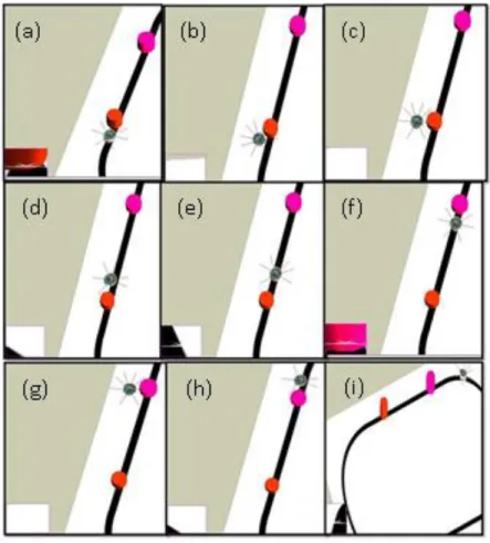
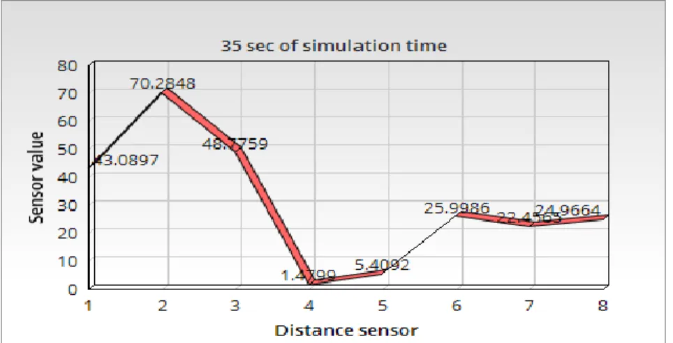
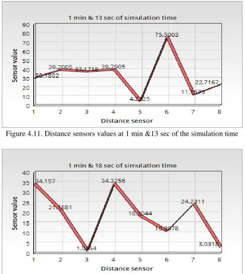
Figure 4.5 Snapshots of the simulation run at different simulation times 42 Figure 4.6 Distance sensors values at 3 seconds of the simulation time 43 Figure 4.7 Distance sensors values at 9 seconds of the simulation time 43 Figure 4.8 Distance sensors values at 35 seconds of the simulation time 44 Figure 4.9 Distance sensors values at 40 seconds of the simulation time 44 Figure 4.10 Distance sensors values at 46 seconds of the simulation time 44 Figure 4.11 Distance sensors values at 1 min &13 sec of the simulation

time

45

Figure 4.12 Distance sensors values at 1 min &18 sec of the simulation time

45

Figure 4.13 All three ground sensors measurements at different simulation times.

47

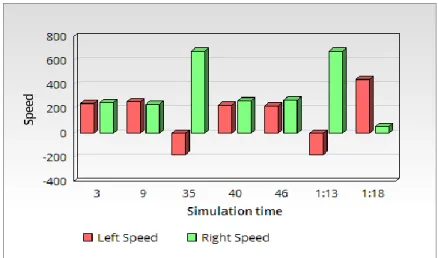
Figure 4.14 Left and right motor speeds 48

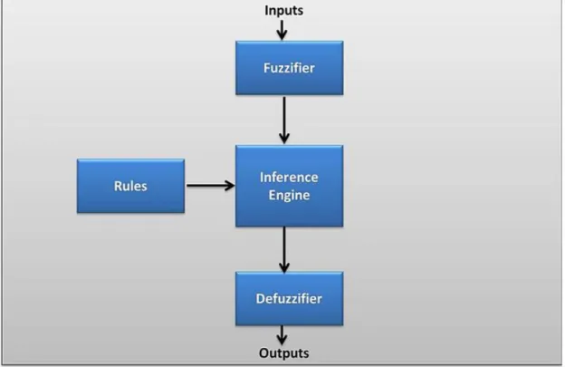
Figure 5.1 Block diagram of Fuzzy Logic System. 52

Figure 5.2 Fuzzy Inference System (FIS) with inputs and outputs. 53 Figure 5.3 Input membership functions for the distance sensors 54

Figure 5.4 Input membership functions for the camera 54

Figure 5.5 Output membership functions. 56

Figure 5.6 Example of the rule editor in MATLAB 57

Figure 5.7 Flowchart of the proposed methodology. 59

Figure 5.8 The E-puck robot with various types of sensors. 60 Figure 5.9 Simulation snapshots of one robot and one obstacle. 61

(18)

xviii

Figure 5.10 Snapshots of the real-time experiment of one robot and one obstacle.

61

Figure 5.11 Simulation snapshots for multiple robots and obstacles 62 Figure 5.12 Real-time experiment for multiple robots and obstacles. 63 Figure 5.13 Distance sensor values for both robots at different simulation

times

68

Figure 5.14 Distance to obstacles for both robots. 69

Figure 5.15 Left and right velocities for both robots at different simulation times.

70

Figure 5.16 Ground sensors values for both robots at different simulation times.

71

Figure 5.17 Traveled distance measured by left and right wheels for both robots

72

Figure 5.18 Simulation overview of the mobile robot and the environment.

73

Figure 5.19 Simulation snapshots at various times. 73

Figure 5.20 Distance sensor values at different simulation times 75 Figure 5.21 Distance to obstacles in meters at different simulation times. 76 Figure 5.22 Ground sensor values at different simulation times. 76 Figure 5.23 Left and right wheel velocities at different simulation times. 76 Figure 6.1 Distance measurements between the robot and the obstacle. 80 Figure 6.2 Average of distance traveled by the robot’s differential 80

(19)

xix wheels.

Figure 6.3 Energy consumption level 80

Figure 6.4 An example of the fusion model at MATLAB’s rules viewer. 81 Figure 6.5 Time complexity of the proposed methodology. 82 Figure 6.6 Average traveled distance by the mobile robot per number of

obstacles.

82

Figure 6.7 Energy consumption level per number of obstacles. 82 Figure 6.8 The comparison of the total number of operations for each

technique.

85

Figure 6.9 The comparison of the average execution time for each technique.

85

Figure 6.10 The comparison of the level of energy consumption for each technique.

(20)

1

CHAPTER 1: INTRODUCTION

There has been a spurt of interest in recent years in the area of autonomous mobile robots that are considered as mechanical devices capable of completing scheduled tasks, decision-making and navigating without any involvement from humans [1], [2]; This has brought up some serious concerns about the interaction between mobile robots and the environment [3]. Due to the increased demand of this type of robot, various techniques and algorithms were developed. Most of them are focused on navigating the robot in collision-free trajectories, with the controlling of the robot’s speed and direction [4].

In contrast to regular robots, an autonomous robot does not know the surrounding environment in advance; hence, it needs to be programmed in a way that it can adjust and be flexible to all changes that occur during operation [5]. Mobile robot motion planning in an unknown environment has always been the main research focus in the mobile robotics area, due to its practical importance and the complex nature of the problem. Several collision avoidance and line following techniques have been introduced lately.

(21)

2

Each of these techniques was developed to be used in specific applications for the purposes of education, entertainment, business, etc [3].

The ability to detect obstacles in real-time mobile robotics systems is a very critical requirement for any practical application of autonomous vehicles. The main objective behind using the obstacle avoidance approach is to obtain a collision-free trajectory from the starting point to the target in monitoring environments. There are two types of obstacles: static obstacle, which has a fixed position and requires a priori knowledge of the obstacle; dynamic obstacle, which does not require any priori knowledge of the motion of the obstacle and has uncertain motion and patterns (moving objects). Indeed, detecting dynamic obstacles is more challenging than detecting static obstacles; the dynamic obstacle has a changeable direction and requires a prediction of the obstacle position at every time step in order to achieve the requirement of a time-critical trajectory planning [6].

In addition, path planning in mobile robots can be divided into two types based on the robot’s knowledge of the environment. Global path planning is where the environmental information is predefined; global path planning is also called static collision avoidance planning. Local path planning is where the environmental information is not pre-known and is also known as dynamic collision avoidance planning. Local path planning is more demanding than global path planning. Local path planning quickly takes into consideration some kinds of measurements regarding the dimensions of the moving obstacle (such as position, size and shape) through sensors to avoid unknown obstacles while the robot is moving towards the goal state [6].

(22)

3

Various methods have been proposed as solutions for line following problems, generally including line-following, object-following, and path tracking, etc. The line follower in robotics is simply an autonomous mobile robot that detects a particular line and keeps following it. This line can be as visible as a black line in a white area or as invisible as a magnetic field [3].

Line following in mobile robots can be achieved in three basic operations. First, capture the line width by camera (image processing) or some reflective sensors mounted at the front of the robot. Second, adjust the robot to follow the predefined line by using some infrared sensors placed around the robot. Third, control the robot speed based on the line condition [3].

1.1 Research Problem and Scope

The development of autonomous mobile robots is still at the center of numerous research projects to provide a collision free path. Given the specific needs required by different applications of mobile robots (especially in navigation), it is crucial to develop an autonomous robotic system that is capable of avoiding obstacles while following a path in real-time applications. Consequently, an efficient collision avoidance and path following technique is essential to assure intelligent and effective autonomous mobile robot systems [3].

These robots need to communicate with the environment through various sensor modules. In the area of autonomous mobile robotics, the most significant tasks are collision avoidance, path planning, and obstacle detection. They autonomously allow the

(23)

4

robot to avoid or mitigate a collision, while traveling in an efficient path towards a desired goal. The robot can be mounted by different kinds of sensors in order to observe the surrounding environment, thus steering the robot accordingly. However, many factors affect the reliability and efficiency of these sensors. The integration of a multi-sensor fusion system can overcome this problem by combining inputs coming from different types of sensors, hence having more reliable and complete outputs; this plays a key role in building a more efficient autonomous mobile robotic system [4].

1.2 Motivation behind the Research

To assure efficiency and robustness, the integration of sensor or data fusion is considered a crucial aspect (especially in real-time systems). Sensor fusion can be defined as the combining process of sensory data in order to generate improved data that assures robustness and confidence, as well as diminishes ambiguity and uncertainty. For the purpose of collision avoidance and path following approaches, different types of sensors (such as camera, infrared sensor, ultrasonic sensor, and GPS) can detect different aspects of the environment. Each sensor has its own capability and accuracy, whereas integrating multiple sensors enhances the overall performance and detection of obstacles [4].

Many data fusion techniques exist such as fuzzy logic, kalman filter, particle filter, Bayesian methods, and the Dempster-Shafer methods. Using one of these techniques or a combination is useful for enhancing the output data. Fuzzy logic is an approach used for sensor fusion with small computational load, especially in unknown environments to avoid faulty interventions resulting from invalid observations. Therefore,

(24)

5

using fuzzy logic to fuse data obtained from different types of sensors boosts the robustness of the algorithm required for collision avoidance and path planning in autonomous mobile robotic systems.

1.3 Contributions of the Proposed Research

The goal of this work is to design and experimentally implement a collision-free path follower robot, with the integration of data fusion. The aim of the fusion system is to enhance the robustness and the efficiency of the algorithm used.

A novel real-time obstacle avoidance and line follower approach for mobile robots has been developed and tested in both simulation and real-time experiments. The proposed technique allows the simultaneous detection of obstacles with the control of the mobile robot to eliminate collisions and recover the path again. The novelty of this technique arises from the integration of data fusion techniques, along with the proposed algorithm for steering the mobile robot. This combination is extremely helpful for obtaining more accurate sensor data, thus enabling the robot to react more efficiently in case of obstacle detection. The performance of the proposed technique has been evaluated using simulated and experimental data. Our framework aims for higher efficiency and accuracy using data fusion, while ensuring overcoming obstacles along the path. In this work, we are mainly concerned about extracting necessary fused sensor data from multi-modality sensors for vigorous collision free trajectory planning approach.

(25)

6

- Design a collision avoidance and line follower framework for a mobile robot.

- The capability of the mobile robot to avoid obstacles along its path, based on the use of infrared sensors.

- The capability of the mobile robot to follow a path.

- An efficient algorithm of the proposed technique is developed.

- The integration of multisensory information from range finder camera and infrared sensors, using fuzzy logic fusion system for collision avoidance and line follower mobile robot.

- The proposed methodology develops membership functions for inputs and outputs and designs fuzzy rules, based on these inputs and outputs. - The performance of the mobile robot when programmed with the fuzzy

logic sets and rules.

- The proposed methodology has been successfully tested in Webots Pro simulator and real-time experiments.

- The proposed methodology has been tested in different levels of complexities with static and dynamic obstacles, using one and multiple robots while avoiding obstacles in different shapes and sizes.

- The proposed methodology reduced the traveled distance of the mobile robot, as well as minimized the energy consumption and the distance between the robot and the obstacle detected as compared to a non-fuzzy logic approach.

(26)

7

CHAPTER 2: LITERATURE SURVEY

2.1 Introduction

Robotic systems need a lot of information about the surrounding environment in order to be able to accomplish the required tasks (such as collision avoidance, line following, or target seeking). This information must be acquired faster, more accurately, and more precisely. Therefore, heterogeneous sensors or many homogenous sensors are used to get useful measurements about the environment. However, data can be redundant and overlapped, which consumes more energy and time. To eliminate this problem, sensor fusion is applied to combine data from different types of sensors to generate more complete data.

Sensors are used to observe the surrounding environment. Sometimes sensors fail to collect accurate data from the environment, due to pressure and temperature. In other cases, this failure can be attributed to electromagnetic noise or radiation. Therefore, all readings and measurement would be inaccurate and inefficient. In order to overcome these problems, data fusion (which is a technique combining data from several sources to be more accurate and complete) is used. Data fusion is applied in centralized systems, as well as in distributed systems [7]. Data fusion can eliminate redundant data and thus save energy, which results in an improved performance [8].

(27)

8

Data fusion has been used in many detection applications such as robotics [9]. Recently, new applications such as Denial of Service (DoS) detection deployed the data fusion concept successfully [10]. Another example is intrusion detection [11].

In relation to the importance of data fusion, this section presents many techniques that have been applied in sensor based systems in general. Our goal is to analyze each technique and evaluate the advantages and the disadvantages of each in order to comprehend the best usability of these techniques in different applications [12].

2.2 Data Fusion Techniques and Methods

Based on the purpose of the method, data fusion techniques can be implemented for a variety of "objectives such as inference, estimation, classification, feature maps, abstract sensors, aggregation, and compression" [13]. In this section, many techniques used in data fusion are discussed along with their applications. Figure 2.1, shows all data fusion techniques.

(28)

9

2.2.1 Inference Methods

Inference method is mostly used in decision fusion where a decision is generated depending on the perceived situational knowledge. "Classical inference methods are based on Bayesian inference and Dempster-Shafer Belief Accumulation theory" [13],[14]. Other inference methods such as fuzzy logic, neural networks, abductive reasoning, and semantic data fusion are also highlighted.

2.2.1.1 Bayesian Inference

Depending on the probability theory, Bayesian Inference merges all evidences where the uncertainty in Bayesian Inference describes the belief. It assumes the value of 0 for absolute disbelief and 1 for absolute belief. Bayesian inference is basically based on the "Bayes’ rule" [15], [13], which is represented in Equation (2.1):

Pr(B | A ) = (Pr(A | B ) * Pr(B )) / ( Pr(A)) (2.1) Where, Pr(B | A ) is the belief of hypothesis B given the information A, Pr(A | B ) is the probability of receiving A, given that B is true, Pr(B ) is the prior probability, and Pr(A) is the normalizing constant.

The critical issue in Bayesian Inference is that the probabilities Pr (A) and Pr (A|B) should be estimated because they are unknown. The neural network approach has been used to guess the conditional probabilities for the decision-making process in Bayesian inference module [16]. In addition, Cou´E et al. [17] used Bayesian programming in fusing data from various sensors such as laser and video in order to obtain more reliable and accurate data.

(29)

10 2.2.1.2 Dempster-Shafer Inference

This method is based on the "Dempster-Shafer Belief", which generalizes the Bayesian theory. Dempster-Shafer Belief was proposed by both Dempster [18] and Shafer [19]. Dempster-Shafer Inference introduces a formalism that is applied for incomplete knowledge and evidence combination [20]. An important factor in Dempster-Shafer method is the set of all possible states which further demonstrates the system. This set is called the ‘frame of discernment’. The elements of the power set of possible states are called hypotheses. Each hypothesis has its assigned probability. In addition, the belief function which is called ‘bel’ is defined by Dempster-Shafer and also the degree of doubt ‘dou’ that is based on the belief function are [21].

2.2.1.3 Semantic Data Fusion

Semantic data fusion is done as an in-network inference. The semantic data fusion method is composed of two important phases. The first phase is called knowledge base construction, which collects the "knowledge abstractions" into a form of semantic data. The second phase is called pattern matching (inference), which uses the semantic data provided by the previous phase to fuse relevant attributes for pattern matching [22]. This method was first introduced by Friedlander and Phoha [22] for target classification. Friedlander [23] explains many techniques that extract semantic data from sensors by converting sensor data into formal languages. He applies these techniques for the recognition of the robots’ behavior and for saving resources.

(30)

11 2.2.1.4 Fuzzy Logic

Fuzzy logic deals with "approximate reasoning" in order to obtain "conclusions from imprecise premises" [24], [7]. Zadeh [25] has introduced the concept of fuzzy sets which later guided him to the fuzzy logic theory. The data fusion algorithm based on fuzzy logic theory has four main phases: "fuzzification", "rule evaluation", "combination" or "aggregation of rules", and "deffuzification" [26]. In the second phase which is the rule evaluation, the implications or rules are used to process the fuzzified inputs. These rules are in the form of “if A then B”, where A is a conditional statement. Sometimes more than two conditional statements are used which is called complex implications. When applying complex implications, fuzzy operators are used for computing the final result [27]. The most common fuzzy logic inference operators used are shown in Equations (2.2), (2.3), (2.4), (2.5), (2.6), (2.7), (2.8), and (2.9) as follows [27]: x⟶y = yx (2.2) x⟶y = min{1,1-x+y} (2.3) x⟶y = min {x,y} (2.4) (2.5) (2.6) (2.7) x⟶y = max { 1-x,y} (2.8)

(31)

12

x⟶y = 1-x+xy (2.9) In Equation (2.4), the Mamdani inference operator is presented. It finds the minimum degree of the membership (x, y). Both Mamdani and Tsukamoto-Sugeno inference methods are based on fuzzy logic [28]. However, the Mamdani method is considered a better method since it ensures an efficient data fusion, extends the sensor lifetime, and reduces delay compared to Tsukamoto method.

In [29], authors use fuzzy logic control and an intelligent sensor network for autonomous navigational robotic vehicle which has the ability of avoiding obstacles. Another implementation of fuzzy logic is for efficient routing that minimizes energy usage [30].

2.2.1.5 Neural Networks

The Neural network is applied in "learning systems" with fuzzy logic to manage its "learning rate" [31], [32], [7]. In the data fusion domain, neural networks have been applied in many applications such as "Automatic Target Recognition (ATR)" [33]. Lewis and Powers [34] fused audio-visual information using neural networks for audio-visual speech recognition.

2.2.1.6 Abductive Reasoning

Abductive Reasoning is the best hypothesis for explaining observed evidence [35]. Figure 2.2 shows the deduction and abduction example. The abductive inference finds the maximum a posteriori probability [36]. Abduction was used in machine learning problems [37] and diagnosis problems [38].

(32)

13

Figure 2.2. The deduction and abduction example.

2.2.2 Estimation Methods

Estimation methods are derived from the control and the probability theories in order to calculate a process vector from a series of measurement vectors [39]. Examples of Estimation methods are Maximum A Posteriori (MAP), Particle filter, Least Squares, Kalman filter, Maximum Likelihood (ML), and Moving Average filter. The details of each method are presented in this section.

2.2.2.1 Maximum A Posteriori (MAP)

This technique is based on Bayesian theory. Given that ‘a’, is the state to estimate, where ‘b’= {b(1),b(2),..,b(n)} is a set of n observations of ‘a’, the MAP estimator is used to figure out a value of ‘a’ in order to maximize the posterior distribution function [40] as in Equation (2.10).

X̂ (n)=arg⁡maxa pdf(a|b) (2.10)

(33)

14

MAP estimator was used by Schmitt et al. [41] in a known environment to locate the joint positions of mobile robots. Another implementation of MAP estimator was by Yuan and Kam [42] in the collision resolution algorithm. The algorithm’s purpose is to control the traffic between the fusion node and the source, where MAP estimator figures out the number of nodes that are being transmitted. Therefore, the retransmission probability of these nodes needs to be updated accordingly.

2.2.2.2 Particle Filter

Particle filters are recursive processes of the "sequential Monte Carlo methods (SMC)" [43]. They are suitable for applications that implement a non-Gaussian noise [44]. They use a large number of random measurements which are composed of particles (samples) that are driven from distributions and weights of the particles. The random measurements are helpful in calculating all kinds of unknown estimates such as minimum mean square error (MMSE) and maximum a posteriori (MAP). The Particle filter technique represents significant densities by particles and weights. It then computes the integrals by Monte Carlo methods. There are three important operations of the Particle filters: sample step that generates particles, importance step that computes the particle weights which are normalized later, and the resampling step. The resampling is important as it eliminates the trajectories with small weights and highlights the ones that are dominating [45].

2.2.2.3 Least Squares

The "Least Squares method is a mathematical optimization technique that searches for a function that best fits a set of input measurements. This is accomplished by

(34)

15

minimizing the sum of the square error between points generated by the function and the input measurements" [7]. Unlike the "Maximum A Posteriori Probability", the Least Square does not use any previous probability. Therefore, it works in a deterministic manner [13]. The Least Squares method tries to find the value of x [40] as in Equation (2.11).

(2.11)

Where h is the sensor model for a sequence of 1 ≤ i ≤ n observations.

An advantage of using the Least Squares method is reducing the communication between the source node and the sink. This is achieved by sharing the sensor data through the linear regression instead of transmitting the actual data [46].

2.2.2.4 Kalman Filter

The Kalman filter was invented by Kalman [47] and it gained popularity as a technique used for data fusion. The Kalman filter is shown in Figure 2.3. Based on some measurement y(n) which is shown in Equation (2.12), and the system parameters (which are known in advance), the estimate of x(n), and the prediction of x(n + 1) are presented in Equations (2.13), and (2.14) respectively.

y(n) = H(n) x(n) + r(n) (2.12) Where: H(n) is the measurement matrix, r is a random variable that follows the zero-mean Gaussian laws.

(35)

16

X̂ (n)= X̂ (n | n-1)+K(n)[y(n)-H(n X̂ (n | n-1)] (2.13) Where K is the Kalman filter gain.

X̂ (n + 1 | n) = Ts (n) X̂ (t | t) + Ti (n) I(n) (2.14) Where: Ts(n) is the state transition matrix, Ti (n) is the input transition matrix, and I (n) is

the input vector.

The Kalman filter technique works well in a linear model where it retrieves optimal estimates recursively [48]. On the other hand, in a nonlinear model, other methods should be used such as "Extended Kalman filter (EKF)" [49], and the "Unscented Kalman Filter (UKF)" [50].

Figure 2.3. Kalman filter block diagram

2.2.2.5 Maximum Likelihood (ML)

To estimate a state ‘a’ as an example, where ‘b’= {b(1),b(2),..,b(n)} is a set of n observations of ‘a’, the likelihood function is defined as follows:

λ(a) = p (b |a) (2.15) Where p is the probability density function.

(36)

17

The Maximum Likelihood estimator (MLE) is used to figure out a value of ‘a’ in order to maximize the likelihood function [40] as in Equation (2.16).

(2.16) A new distributed and localized MLE was proposed by Xiao et al. [51] with more robustness, where each node can compute a "local unbiased estimate" to eventually reach "the global Maximum Likelihood solution" [13]. This method was further developed by Xiao et al. [52] in order to deliver measurements in a timely manner.

2.2.2.6 Moving Average Filter

The moving average filter is mainly used in "digital signal processing (DSP) solutions" [13]. It has many advantages such that it is easy to use as it reduces "random white noise" while maintaining a "sharp step response" [13]. For this reasons it is an optimal filter in the time domain for processing encoded signals [53]. The true signal x = ( (1), (2), . .) is estimated by Equation (2.17).

(2.17) Where z=(z(1), z(2), . . .), is the input digital signal, w is the filter’s window that indicates the number of input observations for every n ≥ w.

In addition, w refers to the number of steps needed for the filter to identify the signal level's variance. As the value of w increases, the signal becomes cleaner. In contrast, as the value of w decreases, the step edge becomes sharper. The Moving Average filter is able to decline √w of the white noise variance [53].

(37)

18

2.2.3 Compression

Compression methods are applied through spatially correlating all sensors with no additional communication cost. This can be obtained by providing two sensors with correlated observations [54]. Several compression methods are discussed in this section.

2.2.3.1 Distributed Source Coding (DSC)

Distributed Source Coding (DSC) [55], is "the compression of multiple correlated sources, physically separated, that do not communicate with each other "[56]. One of the most popular data compression methods is the "Distributed Source Coding Using Syndromes" (DISCUS) framework [57]. In DISCUS, assuming we have a sensor X which wants to transmit its observation to sensor Y. In order to code X’s observation, X can send only an index. There is one requirement which is the Hamming distance between X and Y which is at most one. This means that the difference of X and Y can be only one bit. Suppose that a sensor observation can be any value of the set S={000, 001, 010, 011, 100, 101, 110, 111}. X and Y have four cosets {000, 111}, {001, 110}, {010, 101}, {100, 011}. As shown in Figure 2.4, sensor X sends the index of 10 which corresponds to the coset of {010, 101}. Y now can decode the index along with its own observation of (100). Since the Hammimg distance should be at most one between the two, Y knows that the value provided by X should be 101 [13].

2.2.3.2 Coding by Ordering

This technique was first introduced in Petrovic et al. [58]. In this technique, each node sends the data to the border node. The border nodes are responsible for sending what is called a supper-packet, which is a group of all packets, to the sink node. Table

(38)

19

2.1, gives an example of coding by order. As shown in Table 2.1, we have four nodes that each of them provides an observation of the value from 0 to 5: X,Y,Z, and W. As shown in Table 2.1, the border node can suppress all values by W. The ordering is 3! which means that we have 6 possible orderings of the three remaining nodes: X, Y, and Z. For example, if the observation value for node W is 1, the packet order is {X,Z,Y} where it can be {Z,X,Y} if the observation value for node W is 4 and so on [13].

Figure 2.4. An example of DISCUS data compression.

Table 2.1: Code by ordering example. Packet Ordering Observation Value (W)

{X,Y,Z} 0 {X,Z,Y} 1 {Y,X,Z} 2 {Y,Z,X} 3 {Z,X,Y} 4 {Z,Y,X} 5

(39)

20

2.2.4 Aggregation

According to Kulik et al. [59], data aggregations is defined as a technique that is used for solving two kinds of problems: implosion which occurs when the data sensed are duplicated by the same node because of the strategy used in routing, and overlap which occurs when two different nodes broadcast the same data (redundant sensors) [13]. Redundancy has a negative effect as it wastes the energy. Therefore, data aggregation and data fusion are important to reduce energy consumption. For that specific reason, data aggregation is applied for the purpose of reducing redundancy in neighboring nodes [60], [61]. Using data fusion techniques can decrease the number of packets needed to be transmitted by processing data locally and then send only a digest to the sink node which in return saves energy and bandwidth. To illustrate this, the centralized approach takes O (n3/2) bit-hops, where when applying data fusion techniques it takes only O (n) bit–hops for data transmission [62].

In-network data aggregation algorithms have gained a lot of attention recently since they require coordination among nodes when they are distributed in the network to assure high performance which is basically a complex functionality. In-network aggregation can be defined as collecting and routing data within a "multi-hop network" where it processes data at intermediate nodes in order to decrease energy consumption and thus increase the network’s lifetime [63].

(40)

21

2.2.5 An Information Theory Approach

Using multiple sensors instead of a single sensor in any network can enhance data and observation reliability. Information fusion based on multiple sensors is harder to estimate in advance. This leads to a probabilistic data collection and processing which can be measured and analyzed by applying the information theory principles [64]. Both the "Information" and "Detection" theories help in solving many problems regarding data fusion. Ahmed and Pottie [65] have used a Bayesian technique for fusion which uses different sensor types along with different sensing capabilities.

2.2.6. Reliable Abstract Sensors

This method was first proposed by Marzullo [66] which suggests three different types of sensors: "concrete sensor", which senses the environment by collecting samples of a physical variable, "abstract sensor" which represents the observation in a set of values depending on the concrete sensor, and "reliable abstract sensor" which contains the real values of the physical variable. This type of sensor is computed using a number of abstract sensors. This fusion method has been applied in various applications in time synchronization [67]. Many algorithms and functions are used with reliable abstract sensors for time synchronization such as "Fault-Tolerant Averaging" algorithm and "Fault-Tolerant Interval" (FTI) function.

2.2.6.1 Fault-Tolerant Averaging

This algorithm is used in data fusion methods as it fuses a n number of "abstract sensors" into correct "reliable abstract sensors" even if there are incorrect sensors [66].

(41)

22

The algorithm works as follows. Suppose we have L={I1, . . . , In} where Ii = [xi , yi] by n

abstract sensors at the same time and we have at most f of n abstract sensors which are incorrect or faulty. The "Fault-Tolerant Averaging" algorithm is shown in Equation (2.18) which has a complexity of O(nlog n) [66].

(2.18) Where:

Low refers to the smallest value in at least n − f intervals in L, and High refers to the largest value in at least n − f intervals in L.

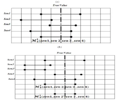
Figure 2.5, shows two different scenarios of applying the Fault-Tolerant Averaging algorithm where there is one faulty sensor. In Figure 2.5 (a) Sen 2 and Sen 3 do not have any intersection; therefore, one of them is the faulty sensor. (sen 1,sen 2,sen 3 ,sen 4) has {Low,High}, where Low (the left edge of Sen 1)= n − f = 4 − 1 = 3, and High (the right edge of Sen 4)= n − f = 4 − 1 = 3. However, in Figure 2.5 (b), the right edge of Sen 2 has moved to the left and becomes Sen 2'.

As a result, we have now (sen1,sen 2',sen 3,sen 4) which indicates the instability of M. Consequently, the left edge of the result is the left edge of Sen 3 (Low value) and the right edge of the result is the right edge of Sen 4 (High value). This algorithm was further extended by Chew and Marzullo [68] where they fuse data from multidimensional sensors.

(42)

23

2.2.6.2 Fault-Tolerant Interval Function

This function was introduced by Schmid and Schossmaier [69]. The Fault-Tolerant Interval (FTI) function is also used in data fusion methods. Again, we have at most f of n abstract sensors considered as incorrect or faulty sensors. FTI function is shown in Equation (2.19).

(L)={Low,High} (2.19) Where: Low refers to the (f + 1)th largest of the left edges {x1, . . . , xn}

High refers to the (f + 1)th smallest of the right edges { y1, . . . , yn}

FTI function indicates that when there are few alterations in the input intervals, unlike the Fault-Tolerant Averaging algorithm, the result will include only few changes as well. As a result, the FTI function is more robust as compared to the Fault-Tolerant Averaging algorithm [69].

Figure 2.6 shows the same example as Figure 2.5; however the result is not that affected when Sen 2' is moved (Figure 2.6(b)). Therefore, FTI obviously is less vulnerable to small alterations in the input intervals as compared to the Fault-Tolerant Averaging algorithm [69].

2.2.7 Feature Maps

Sometimes using raw sensory data are not sufficient especially in guidance and resource management applications. As a result, some features that well describe the environment need to be extracted [14]. Many data fusion methods of inference and

(43)

24

estimation produce a feature map. There are two feature maps which are occupancy grid and network scans.

Figure 2.5. Two different scenarios of applying the "Fault-Tolerant Averaging" algorithm where there is one faulty sensor.

(44)

25 2.2.7.1 Occupancy Grid

Occupancy maps define a 2D/3D representation of the space which is organized in square cells where every cell has an estimate that indicates its probabilistic occupancy [70]. This probability is calculated by using multiple types of sensors and various data fusion techniques [71]. Occupancy maps are used in many applications such as robot perception [72], the location's estimation [73], and navigation [74].

2.2.7.2 Network Scans

Network Scans are kinds of activity maps. They also give an overview of the resource distribution in the network [75]. One of the most popular network scans is called eScan [75] which provides information about the remaining energy in the network. The algorithm forms an aggregation tree where each node calculates its local eScan and then sends it to the sink. If two or more eScans are received at the same node, an aggregation process is involved to identify the remaining energy of nodes in a specific region. Finally a map is generated [75].

2.3 Evaluation and Comparison of Data Fusion Techniques

This section evaluates all the data fusion techniques and draws a conclusion about which technique is most suitable and reliable to be applied.

Both the "Bayesian Inference" and the "Dempster-Shafer" theories are well-known Inference methods. Dempster-Shafer method generalizes Bayesian Inference. However, "Dempster-Shafer theory" is a more flexible method than "Bayesian Inference" due to its capability to fuse data from various types of sensors unlike Bayesian Inference

(45)

26

[63]. Another difference between these two techniques is that Dempster-Shafer theory does not require assigning apriori probabilities to unknown propositions [14]. In contrast, Dempster-Shafer involves longer calculations [76]. In addition, Fuzzy logic method is best suitable for decision making with uncertain information from multiple sensors. It also improves the quality of information [27]. On the other hand, fuzzy logic cannot solve problems without the knowledge of an expert as it does not have the learning membership function either during solving the problem or after the problem has been solved [77].

Applying neural network has many advantages. In neural network, data fusion is done closely to the source node which results in enhancing its performance. The algorithm used in neural network draws the important features of data and can be adjusted to meet the requirement of various applications [78]. It also provides robustness to handle many issues like noise [79]. It identifies various signals and reduces the errors and false alarm rate of the sensors in an efficient manner [80]. However, many issues need to be considered during the implementation of a neural network such as the problem of local extremum, misclassification due to data dimension increase, and convergence speed of the training [81]. Abductive Reasoning is another technique which works for pattern reasoning more than a data fusion method. It has been used successfully in fault diagnosis and event detection [13]. The semantic data fusion technique has the ability to improve resource utilization especially when collecting and processing data [13]. This method also reduces transmission cost because the nodes transmit formal language structure without the need of transmitting raw data. On the other hand, this technique

(46)

27

requires in some scenarios a known set of behaviors in advance, which is a difficult process in specific situations [82].

Moreover, when the state that needs to be estimated is not based on some random variables, the Maximum Likelihood (ML) technique is suitable to be applied. It also finds the value of this state and assumes it is fixed. In contrast, the "Maximum A Posteriori" (MAP) technique does not consider that the state’s value is fixed. On the other hand, it takes it as the result of some random variables with known prior pdf [40]. In addition, the "Least Squares" technique is more accurate and suitable to be applied where the state is fixed. This technique does not use any previous probability as compared to the Maximum A Posteriori (MAP) technique [13]. The Moving Average Filter technique can be used to decrease the random white noise. It has also been used to reduce the errors caused by tracking applications [83]. The downside of this technique is that an old value will have the same impact as the most recent measurement which will affect the final result [84]. Kalman filter is an important and powerful technique as it can estimate past, present, and future states [49]. The Kalman filter can be unstable due to the "critical value for the arrival rate of the observations" [85].

Furthermore, Particle filter is an excellent technique used to overcome some difficult problems such as signal processing, navigation, communications, and computer vision. On the other hand, it has some drawbacks as it is considered a complex technique that has a computational intensity [45].

In addition, even though Occupancy grids show only a restricted class of maps which indicate incorrect independence assumptions in prior and posterior distributions,

(47)

28

they also have the advantage of being simply applied [86]. The network scan technique can be helpful in describing network resources and activity. In particular, eScan can guide designers where to deploy new sensors since it presents low energy regions [75]. Moreover, the Fault-Tolerant Averaging technique can successfully fuse n number of abstract sensors into correct reliable abstract sensors where in fact there are incorrect original sensors [66]. However, few alterations in the input intervals can affect the performance of the "Fault-Tolerant Averaging" algorithm [66]. On the other hand, the Fault-Tolerant Interval Function is more robust due to the fact that few alterations in the input intervals will lead to only few alterations in the output [69]. The aggregation technique helps to eliminate redundancy and traffic load which saves energy. However, by using this technique, the fusion node can be compromised by malicious attackers which affect the correctness of the fusion data. Another disadvantage of this technique is that there might be multiple copies of the same fusion results at the sink node which increases the energy consumption at the sink node [87]. Distributed Source Coding (DSC) has the advantage of making the coding decisions process works efficiently separated from the routing process. On the other hand, it requires more computational complexity. It also needs to collect some data from joint statistics which is not an easy task [63]. The Code by Ordering technique is simple but does not present all possible correlations between sensors [13]. Finally, the information theory approach is suitable for analyzing many problems regarding data collection and processing by multiple sensors [64].

(48)

29

Table 2.2, summaries the advantages and the disadvantages of all data fusion techniques [12]. Based on previous findings, we evaluate the various data fusion techniques discussed in this section and draw a closure [12]. To conclude, there are various data fusion techniques that have been applied. However, some of these techniques do not concern the specific requirements of wireless sensors in robotic applications such as low energy consumption and flexibility. Therefore, for the best applicability of data fusion using wireless sensors in robotic applications, some techniques outweigh others as follows [12]:

• The Dempster-Shafer is a good technique as it fuses data sensed by different types of sensors which are needed in many applications.

• The fuzzy logic technique performs very well in the decision making process and has better data quality.

• Neural networks enhance the process of data fusion which is an advantage as it saves power consumption.

• The Semantic data fusion technique saves resources. • The Least Squares technique has high accuracy.

• The Moving Average Filter technique decreases the chances of errors which also saves a lot of energy and thus increases the performance. • The Network scan (eScan) can show low power regions in order to fill in

(49)

30

• The aggregation technique eliminates redundant data and thus saves energy.

Table 2.2. Comparison of data fusion techniques. Data Fusion

Technique Advantages Disadvantages

Bayesian

Inference  More accurate than Dempster-Shafer technique

 Does not fuse data from various types of sensors

 Needs to assign apriori probabilities to unknown propositions

Dempster-Shafer

 Generalizes Bayesian Inference technique

 Flexible technique because it has the ability to fuse data from various types of sensors

 Does not assign apriori probabilities to unknown propositions

 Less accurate technique as compared to Bayesian Inference

 Longer calculations involved

Fuzzy Logic  Effective data fusion technique due to its ability of enhancing the data quality.

 Needs the knowledge of an expert to solve the problem

 Learning the membership function is difficult during or after solving the problem

Neural Network

 Enhance the performance of data fusion because it is done closely to the source node

 The neural network’s algorithm is adjustable to the application requirements.

 Efficiently decreases the errors and false alarm rate of the sensors

 Many issues need to be solved such as local extremum,

misclassification, and convergence speed of the training.

Abductive

Reasoning  Successfully used in fault diagnosis and event detection

Semantic Data

Fusion _ Improves resource utilization Reduces transmission cost

 Requires a known set of behaviors in advance, which is a difficult process in specific situations.

Maximum Likelihood (ML)

 Suitable when the state is not a random variable

 Does not require the sharing of all data Maximum A

Posteriori (MAP)  The state’s value is the result of some random variables with known prior pdf

Least Squares  Does not use any prior probability as compared to the Maximum A Posteriori (MAP) technique. Moving

Average Filter

 Decreases the random white noise

 Reduces the errors caused by tracking applications.

 The final result can be easily affected as the old value will have the same impact as the most recent measurement.

(50)

31

Kalman Filter

 Estimates past, present, and future states.

 It needs clock synchronization which can impact its performance

 Unstable due to the critical value found for the arrival rate of the observations

Particle Filter

 Can solve some difficult problems such as signal processing, navigation,

communications, and computer vision.  A complex technique that has a computational intensity

Occupancy Grids

 Can be simplybe applied

 Shows only a restricted class of maps which presents incorrect independence assumptions.

Network Scan

 Describes the network resources and activity.

 eScan can guide designers as to where to deploy new sensors as it

demonstrates low energy regions

 If two or more eScans are received at the same node, an aggregation process is required in order to determine the remaining energy of the nodes.

Fault-Tolerant Averaging

 Fuses several abstract sensors into correct reliable abstract sensors where in fact these abstract sensors are incorrect original sensors.

 The performance can be affected by few alterations in the input intervals

Fault-Tolerant Interval

 More robust than the Fault-Tolerant Averaging technique because few alterations in the input intervals will result in few alterations in the output

Aggregation

 Eliminates redundancy and traffic load

 Saves energy.

 The fusion node can be compromised by malicious attackers which affect the correctness of the fusion data. Distributed

Source Coding (DSC)

 making the coding decisions process works efficiently separated from the routing process

 Requires more computational complexity.

 Collects some data from joint statistics which is not an easy task Code by

ordering

 Simple technique _

Does not present all possible correlations between sensor nodes Information

Theory Approach

 Analyzes problems in data collection and processing by multiple sensors.

(51)

32

CHAPTER 3: ROBOTIC PLATFORM

Deploying autonomous mobile robots is coupled with the use of external sensors that assist in detecting obstacles in advance. The mobile robot uses these sensors to receive information about the tested area through digital image processing or distance measurements to recognize any possible obstacles [88]. Several ways of testing the surroundings have been introduced in the literature of path planning of mobile robots. Although ultrasonic sensors, positioning systems, and cameras are most widely used to move in an unknown environment, they are not the most suitable solution to facilitate the robot. Therefore, some infrared sensors are used to follow an optimal non-collision path from source to destination, according to particular performance objectives [89].

The most well-known sensors used to follow a specific path while detecting obstacles and measuring the distance between robots and objects are infrared, ultrasonic, and laser sensors [3].

Obstacles detected can be moving or static objects in known or unknown environments. In addition, the path planning behavior can be categorized as global path planning (where the environment is entirely known in advance), or local path planning

(52)

33

(where the environment is partly known or not known at all). The later case is called dynamic collision avoidance [90].

3.1 Robot and Environment Modeling

Using simulations to test the proposed technique is very useful, prior to investigations with real robots. They are more convenient to use, less expensive, and easier to setup. In this work, Webots Pro simulator is used to develop a line follower and collision avoidance environment. It is one of the most well-known simulation software used in mobile robots that is developed by Cyberbotics [91].

It is a Graphical User Interface (GUI), which creates an environment that is suitable for mobile robot simulation. It also allows the creation of obstacles in different shapes and sizes. The mobile robot used in Webots Pro simulator is called the E-puck robot, which is equipped with a large choice of sensors and actuators (such as camera, infrared sensors, GPS, and LED sensors) [91].

The environment is modeled with a white floor that has a black line, in order for the robot to follow it. It also has solid obstacles, which the robot should avoid them. The environment in Webots Pro is called “world”; a world file can be built using a new project directory. Each project file is composed of four main windows (as shown in Figure 3.1): the Scene tree represents a hierarchical view of the world, the 3D window demonstrates the 3D simulation, the Text editor has the source code (Controller), and the Console shows outputs and compilation [91].

(53)

34

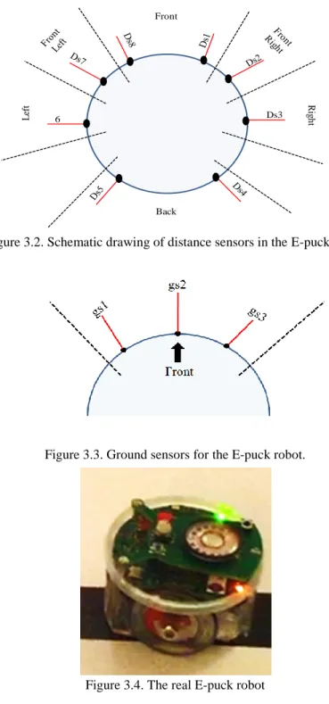
The distance sensors used for collision avoidance are 8 infrared sensors placed around the robot. Figure 3.2 shows a semantic drawing of the top view of the robot used in this work, which is the “E-puck” robot. The red lines represent the directions of infrared distance sensors. For simplicity purposes, we grouped all sensors based on their positions [3].

Figure 3.1. Webots Pro simulator overview

Moreover, the robot detects the obstacles based on the values returned by these sensors, that ranged between 0 and 2000; the values returned from distance sensors depend on the distance between the robot and the obstacle. In other words, the values returned will be 0 ( no light) if there is no obstacle detected and 1000 means obstacle is too close to the robot (big amount of light is measured). For the line-following approach, another type of infrared sensor called ground sensors is used. They are three proximity

(54)

35 Ds3 6 Front Back L eft Ri gh t

sensors mounted on the frontal area of the robot and pointed to the ground, in order to detect the line as shown in Figure 3.3. These sensors allow the robot to see the color level of the ground at three locations in the line across its front [3]. Figure 3.4 shows the real E-puck robot.

Figure 3.2. Schematic drawing of distance sensors in the E-puck robot.

Figure 3.3. Ground sensors for the E-puck robot.

(55)

36

CHAPTER 4: TRAJECTORY PLANNING AND COLLISION

AVOIDANCE ALGORITHM FOR MOBILE ROBOTICS

SYSTEM

This section presents the results of research aimed to develop a new technique for line following and obstacle avoidance, relying on the use of infrared sensors. The sensors involves a reasonable level of calculations, so that it can be easily used in real-time control applications with microcontrollers [3].

4.1 Proposed Technique: Architecture and Design

In this brief, a fairly general technique is developed that has components of formation development, line follower and obstacles detection. The block diagram of the proposed technique is given in Figure 4.1 [3].

The controller receives input values directly from the infrared sensors. The robot controller applies the line follower (LFA) and collision avoidance (CAA) approaches. The (LFA) receives ground sensor readings as input values, then the controller will then issue a signal to the robot to adjust the motor speeds and follow the line; whereas the collision avoidance approach (CAA) receives distance sensor readings as an input value.

(56)

37

When an object is detected in front of the robot, CAA is responsible to spin the robot’s direction and adjust its speed (according to the obstacle's position) in order to avoid collision. By applying both approaches, the robot follows the line and detects obstacles simultaneously. In other words, if an obstacle is detected, the robot must spin around the obstacle until it finds the line again [3].

Figure 4.1. Block diagram of the proposed technique.

An efficient algorithm of the proposed technique is developed (as in Figure 4.2), to make the robot have the ability to follow the path and avoid obstacles along its way [3].

As shown in Figure 4.2, initialization is needed for the global variables that includes the number of distance and ground sensors used (8 distance sensors and 3 ground sensors) and the collision avoidance threshold value prior to starting the line follower and collision avoidance robot. After identifying the number of sensors used for each type, enabling these sensors is the next step [3].